

Learn INT4 quantization techniques for LLMs. Covers group-wise quantization, NF4 format, double quantization, and practical implementation with bitsandbytes.

This article is part of the free-to-read Language AI Handbook
Choose your expertise level to adjust how many terms are explained. Beginners see more tooltips, experts see fewer to maintain reading flow. Hover over underlined terms for instant definitions.
INT4 Quantization
Reducing weights from 16 bits to 8 bits cuts memory in half while preserving most model quality. The natural question is: can we go further? INT4 quantization promises to halve memory again, fitting a 70B parameter model into roughly 35GB instead of 70GB. But moving from 8 bits to 4 bits isn't just "more of the same." It introduces fundamental challenges that require new techniques to overcome.
As we discussed in the previous chapter on INT8 quantization, the basic idea of quantization is mapping continuous floating-point values to a discrete set of integers. INT8 gives us 256 possible values. INT4 gives us only 16. This dramatic reduction in representational capacity means that naive 4-bit quantization destroys model quality. The techniques we explore in this chapter, particularly group-wise quantization and specialized 4-bit formats, make aggressive quantization practical.
The Challenge of 4-Bit Precision
With only 4 bits, we can represent just 16 distinct values. To understand why this limitation is so severe, consider the fundamental mathematics at play. If we use signed integers, this gives us a range from -8 to 7 (or -7 to 7 with a symmetric scheme). Every weight in a neural network, regardless of its original floating-point precision, must map to one of these 16 values. This is a very coarse discretization of the original continuous space.
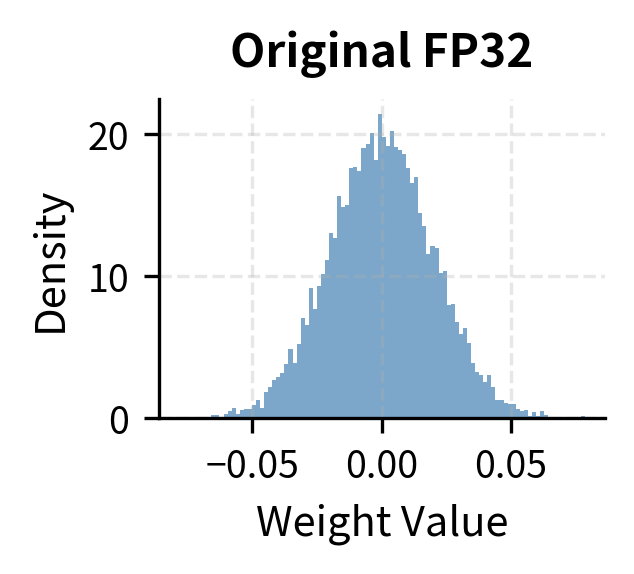
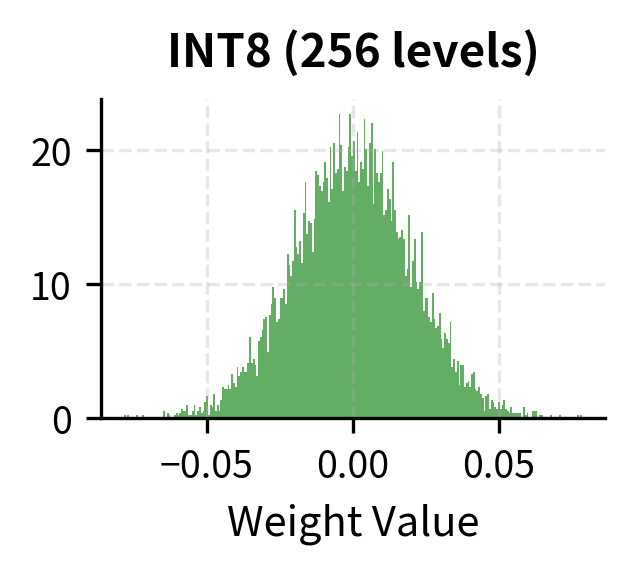
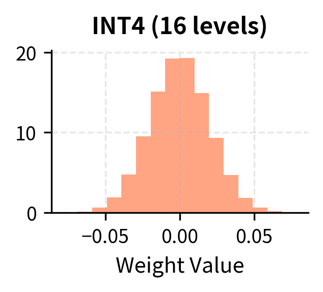
Consider what this means for a typical weight distribution. Neural network weights after training often follow an approximately normal distribution centered near zero. The majority of weights cluster around small magnitudes, with the distribution tapering off symmetrically toward the tails. With INT8, we have enough resolution to capture the shape of this distribution reasonably well, since 256 quantization levels can provide fine granularity even in the densely populated region near zero. With INT4, we're essentially creating a 16-bucket histogram to represent a continuous distribution. Each bucket must absorb a wide swath of the original weight values, collapsing potentially meaningful differences into a single quantized output.
When we quantize a value, we introduce a quantization error equal to the difference between the original value and its quantized representation. With 256 levels, the maximum error for any single weight is bounded by half the step size between adjacent levels. With only 16 levels, that step size becomes 16 times larger, and the maximum quantization error grows proportionally. This error propagates through every matrix multiplication in the network, accumulating and potentially compounding in ways that can fundamentally alter the model's behavior.
The loss of precision becomes more severe when we consider outliers. Recall from our INT8 discussion that neural networks often have a small number of outlier weights with magnitudes much larger than the majority. These outliers, though rare, can be critically important for the model's computations, often encoding strong feature responses or essential biases. With INT8, we can absorb some outlier impact because we have 256 levels to work with, providing reasonable resolution even after accommodating extreme values. With INT4, outliers become catastrophic because the limited number of levels cannot simultaneously span a wide range and maintain adequate precision.
The Outlier Problem Intensified
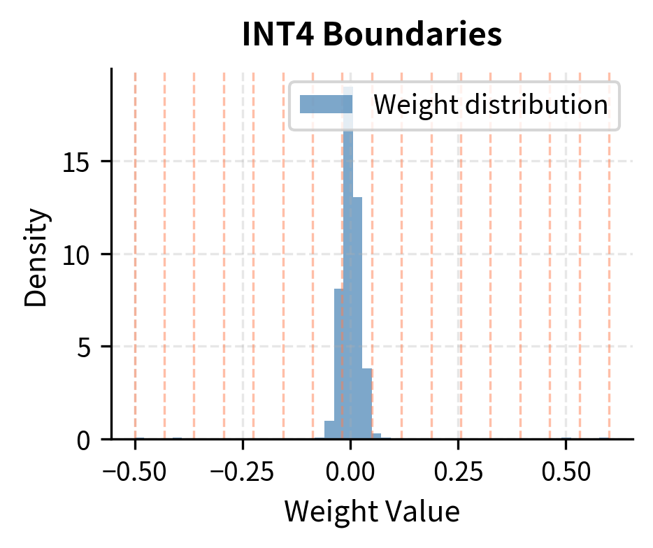
To build intuition for why outliers cause such severe problems at 4-bit precision, imagine a layer where 99% of weights fall between -0.1 and 0.1, but a few outliers reach values of 0.5 or higher. If we set our quantization range to cover the outliers, most of our 16 quantization levels will be "wasted" on the outlier range, leaving very few levels to distinguish the majority of weights near zero. This is a fundamental trade-off that becomes increasingly painful as the number of available levels decreases.
Consider the mathematics of this trade-off. Suppose our 16 quantization levels must span from -0.5 to 0.5 to accommodate outliers. The step size between adjacent levels is then 1.0 divided by 15 (since we have 16 levels creating 15 intervals), giving approximately 0.067 per step. For the 99% of weights living in the range of -0.1 to 0.1, this means they have access to only about 3 distinct quantization levels. The subtle differences between small weights, which are important for model computations, are lost.
With a scale of approximately 0.07, each quantization step is large relative to our typical weights near zero. Most small weights get mapped to the same few quantization levels, destroying the subtle differences between them. The quantization process discards the details that distinguish small weights, even though these differences affect inference.
Group-Wise Quantization
The solution to the outlier problem at 4-bit precision is group-wise quantization, also called block-wise quantization. This technique represents a fundamental shift in how we approach the quantization problem. Instead of using a single scale factor for an entire tensor or even a channel, we divide weights into small groups and compute separate scale factors for each group. This localized approach isolates the impact of outliers, preventing them from corrupting the quantization of the entire weight matrix.
The Group Quantization Concept
To understand why group-wise quantization works so effectively, consider the spatial distribution of outliers within a weight tensor. In trained neural networks, outliers typically don't occur uniformly throughout a tensor. Instead, they appear sporadically, concentrated in certain locations while leaving vast regions of the tensor relatively outlier-free. By using small groups, an outlier affects only the quantization of its own group, not the entire layer. The remaining groups, free from outlier contamination, can use their 16 quantization levels efficiently to represent their local weight distribution with high fidelity.
For a weight tensor, group-wise quantization proceeds through the following steps:
- Divide the weights into groups of size , where common choices are 32, 64, or 128 elements per group
- Compute a separate scale factor (and optionally zero-point) for each group based only on the weights within that group
- Quantize each group independently using its own scale factor
The key insight is statistical: within any sufficiently small group of weights, the probability of encountering an extreme outlier is much lower than across the entire tensor. When an outlier does appear in a group, it affects only the weights in that group, leaving the thousands or millions of other weights in the tensor unaffected. Containing outlier damage makes 4-bit quantization practical.
Smaller groups provide better quantization accuracy because outliers affect fewer weights. However, smaller groups require storing more scale factors, increasing memory overhead. A group size of 128 is common, adding roughly 0.125 bits per weight in overhead (one FP16 scale per 128 4-bit weights). Choosing a group size involves balancing accuracy and storage. The best choice depends on the model and memory.
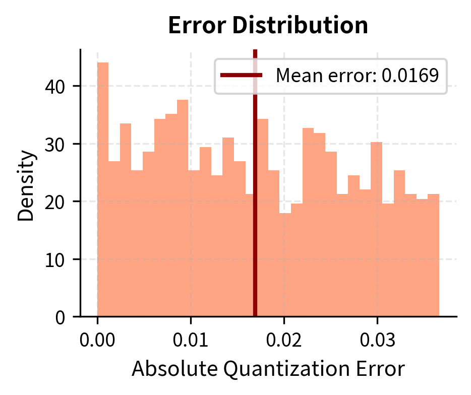
Now let's compare uniform quantization versus group-wise quantization on our weights with outliers. This comparison will demonstrate the dramatic improvement that group-wise quantization provides when outliers are present in the data.
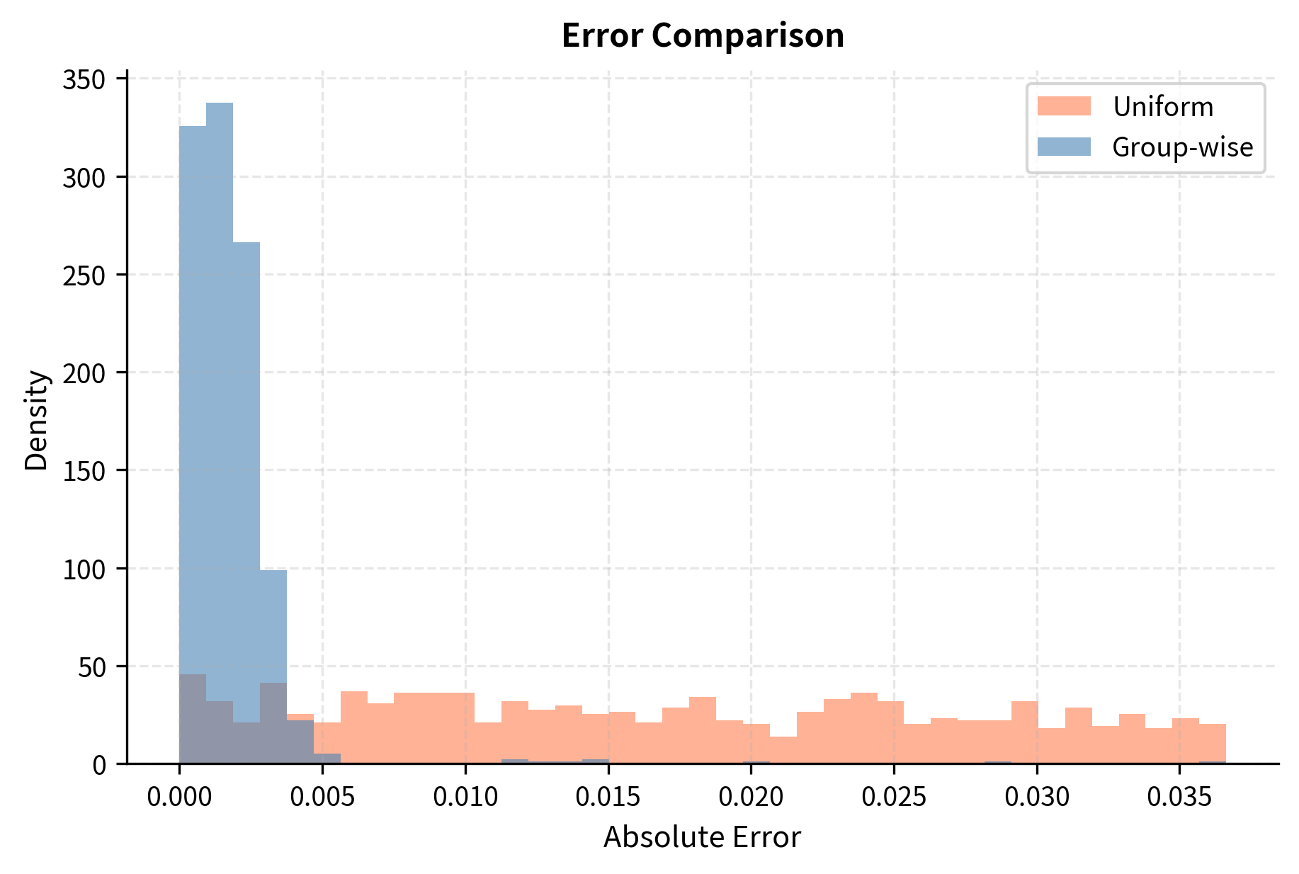
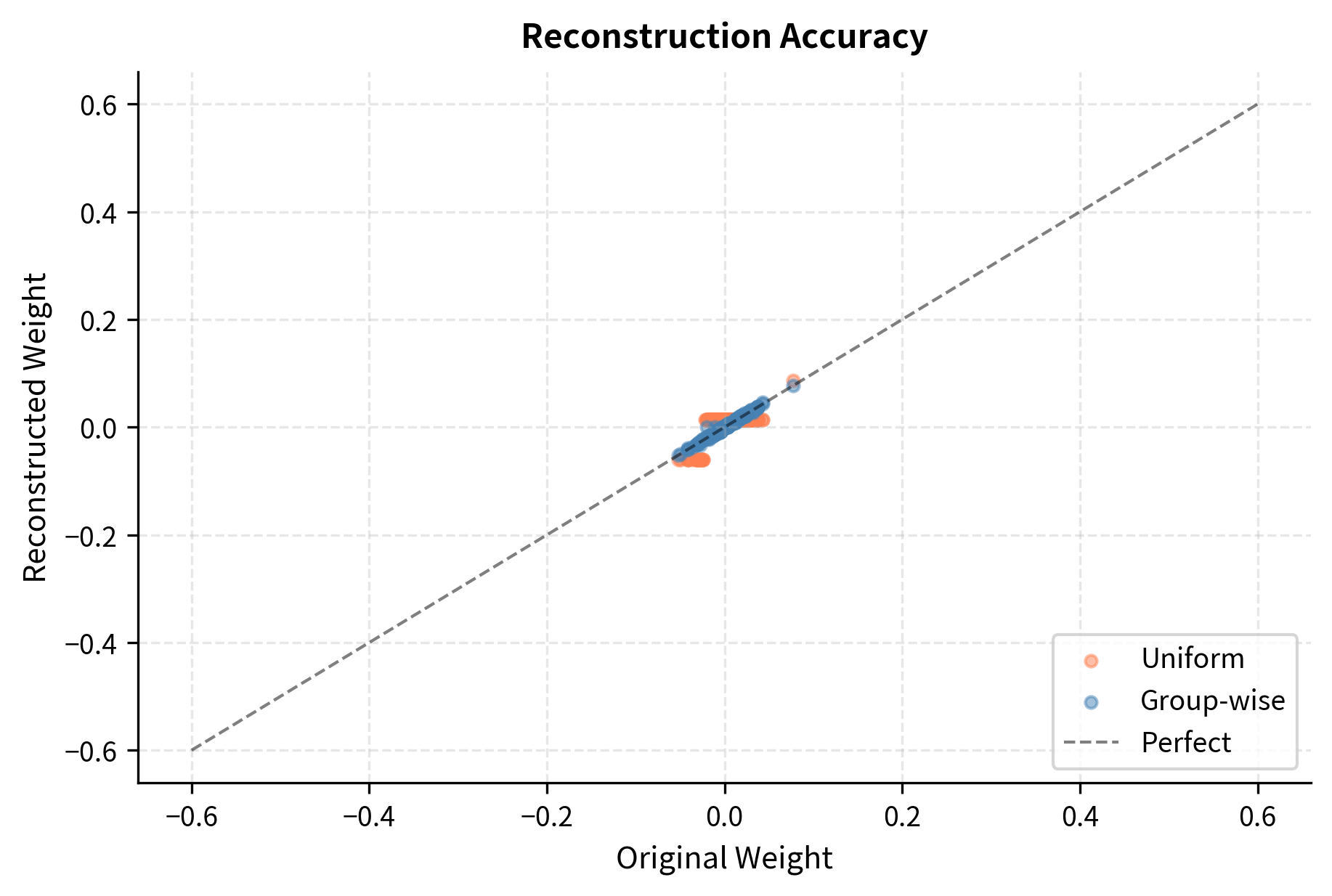
Group-wise quantization dramatically reduces quantization error because outliers no longer dominate the scale factor for the majority of weights. Each group operates with a scale factor tailored to its local distribution, ensuring that the 16 available quantization levels are deployed where they provide the most benefit for that particular subset of weights.
Optimal Group Size Selection
The choice of group size balances accuracy against memory overhead, and understanding this trade-off is essential for making informed deployment decisions. Smaller groups provide finer-grained adaptation to local weight statistics, but each group requires its own scale factor. These scale factors, typically stored in FP16 format (16 bits each), add to the overall memory footprint. Let's examine this trade-off quantitatively:
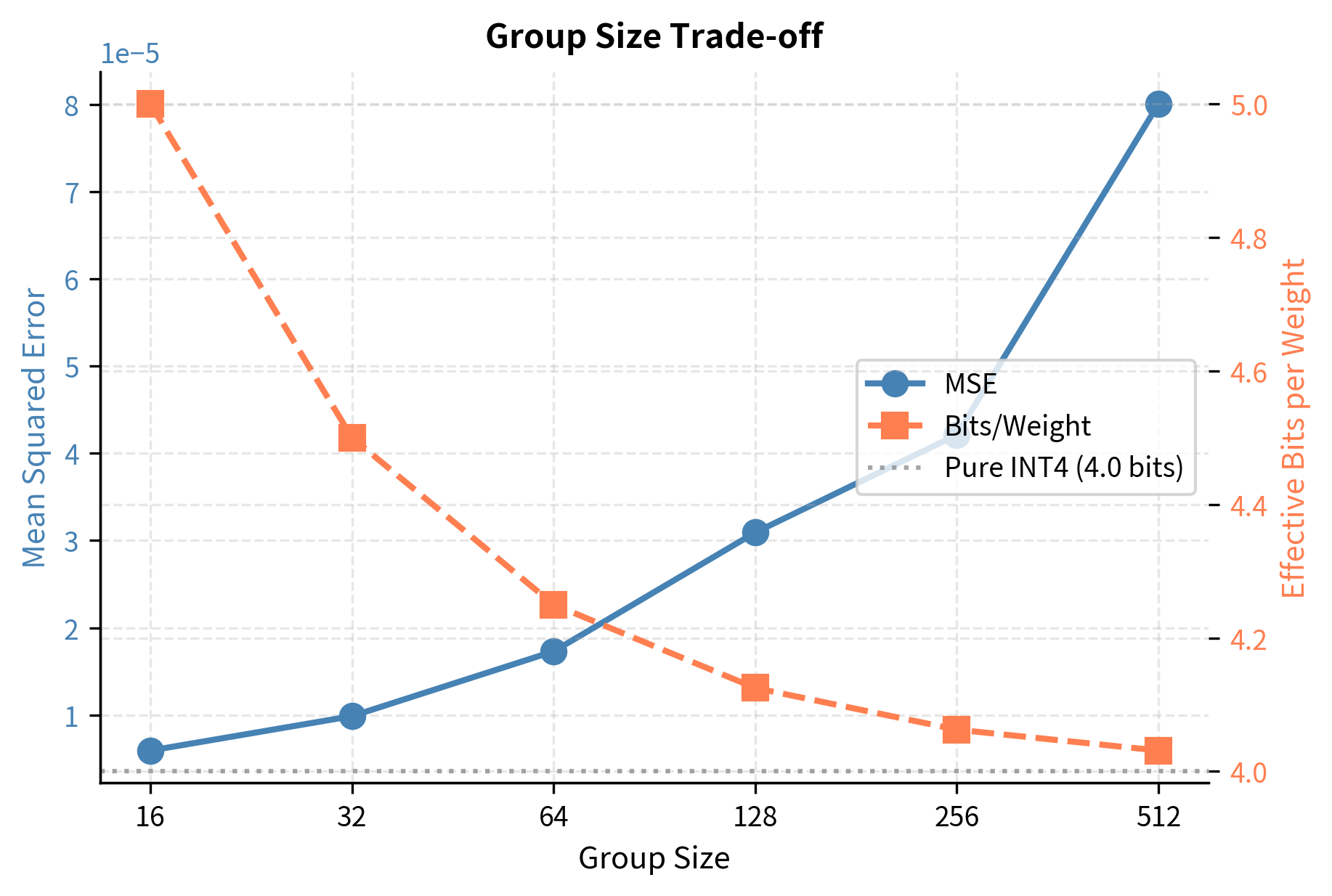
Group sizes of 32-128 typically offer the best balance between quantization fidelity and storage efficiency. Smaller groups provide diminishing returns in accuracy while significantly increasing the number of scale factors to store. The sweet spot depends on the specific model and hardware constraints, but 64 or 128 elements per group has emerged as a common choice in practice, providing good accuracy with manageable overhead.
4-Bit Number Formats
Not all 4-bit formats are the same. Your choice significantly affects model quality. The standard INT4 format, while simple and well-understood, may not be optimal for neural network weights. Several specialized 4-bit formats have been developed to better match the statistical properties of weight distributions, each with its own trade-offs between representational efficiency and computational convenience.
Standard INT4
Standard INT4 uses 4 bits to represent integers in a fixed range. The simplicity of this format makes it computationally efficient and easy to implement:
- Unsigned INT4: Values 0 to 15, representing 16 non-negative integers
- Signed INT4: Values -8 to 7 (or -7 to 7 for symmetric quantization around zero)
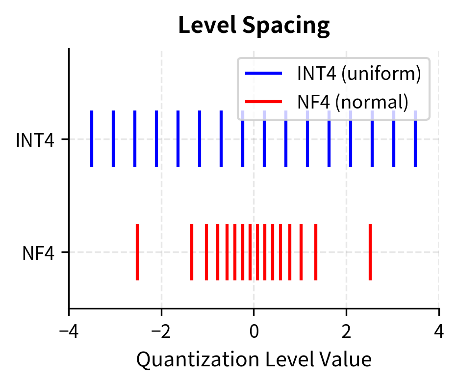
The quantization levels in standard INT4 are uniformly spaced across this range, meaning adjacent levels differ by exactly the same amount regardless of where they fall in the range. For neural network weights that follow a roughly Gaussian distribution, this uniform spacing wastes representational capacity. The problem is one of mismatch between the format and the data. Many quantization levels fall in the tails of the distribution where few weights exist, while the dense center region near zero has too few levels to capture the subtle variations among the many weights clustered there.
NF4 (Normal Float 4)
NF4, introduced alongside QLoRA (which we covered in Part XXV), represents a fundamentally different approach to 4-bit representation. Rather than accepting uniform spacing as a given, NF4 is specifically designed for normally distributed data. Instead of uniform spacing, NF4 places quantization levels such that each level represents an equal probability mass under a standard normal distribution.
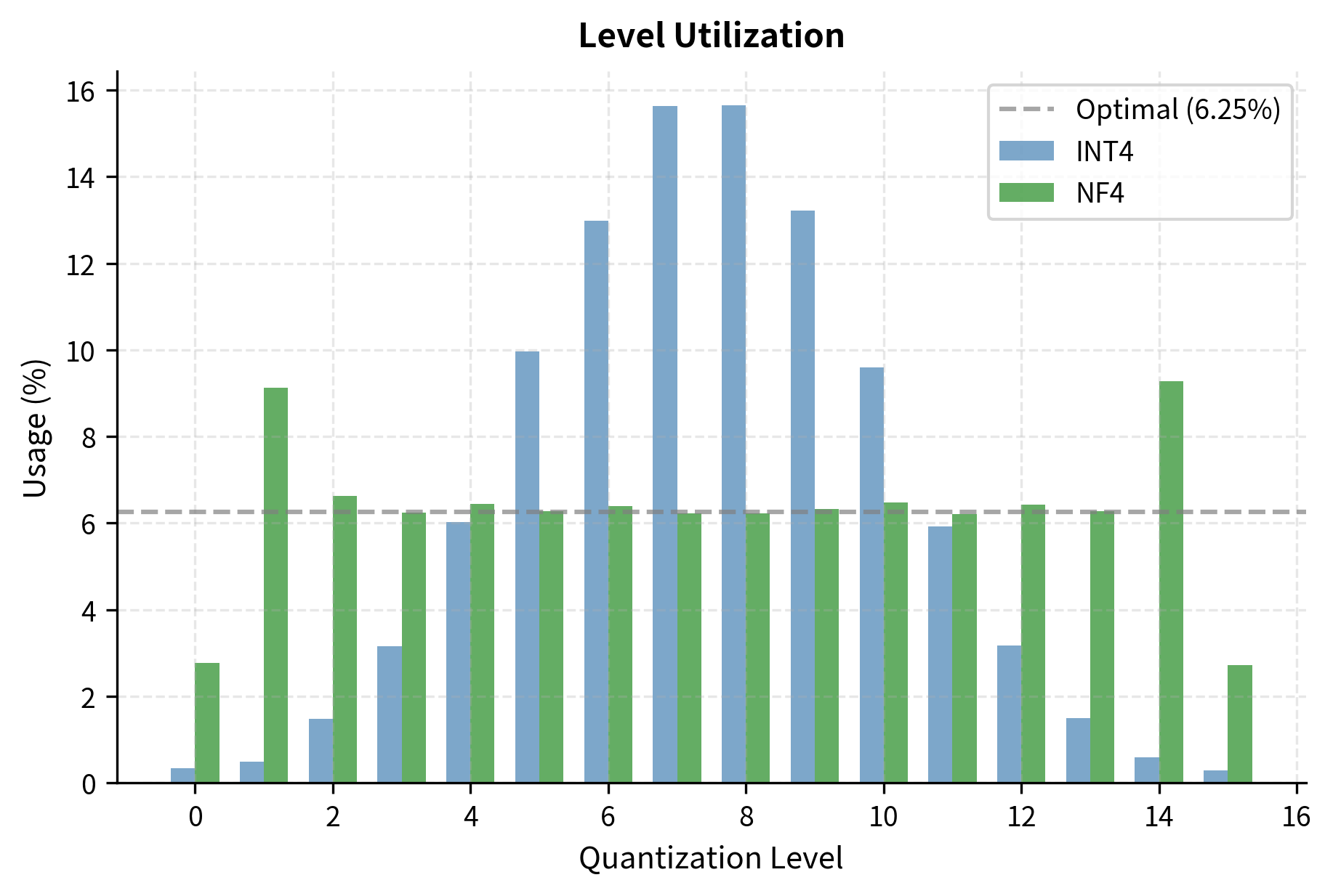
NF4 chooses its 16 quantization levels so that when weights are normally distributed, each level is equally likely to be used. This maximizes information entropy and minimizes expected quantization error for Gaussian-distributed weights. The mathematical foundation for this approach comes from information theory: by ensuring each quantization level is equally probable, we extract maximum information from our limited 4-bit budget.
The NF4 quantization levels are computed through a principled mathematical procedure. The core idea is to find the 16 quantiles of the standard normal distribution that divide it into 16 regions of equal probability, then use the midpoint of each region as the quantization level. This ensures that, for normally distributed data, approximately 6.25% of weights (one-sixteenth) will map to each quantization level, achieving optimal utilization of all available levels.
Notice how the NF4 levels are denser near zero, where most weights concentrate, and sparser in the tails where weights are rare. This non-uniform spacing is the key innovation: by allocating more quantization levels to the regions where data is abundant, NF4 reduces average quantization error compared to uniform spacing. The levels near zero differ by small amounts, allowing fine discrimination among the many similar small weights. The levels in the tails differ by larger amounts, but this matters less because few weights fall there. Let's visualize this relationship between the quantization levels and the underlying distribution:
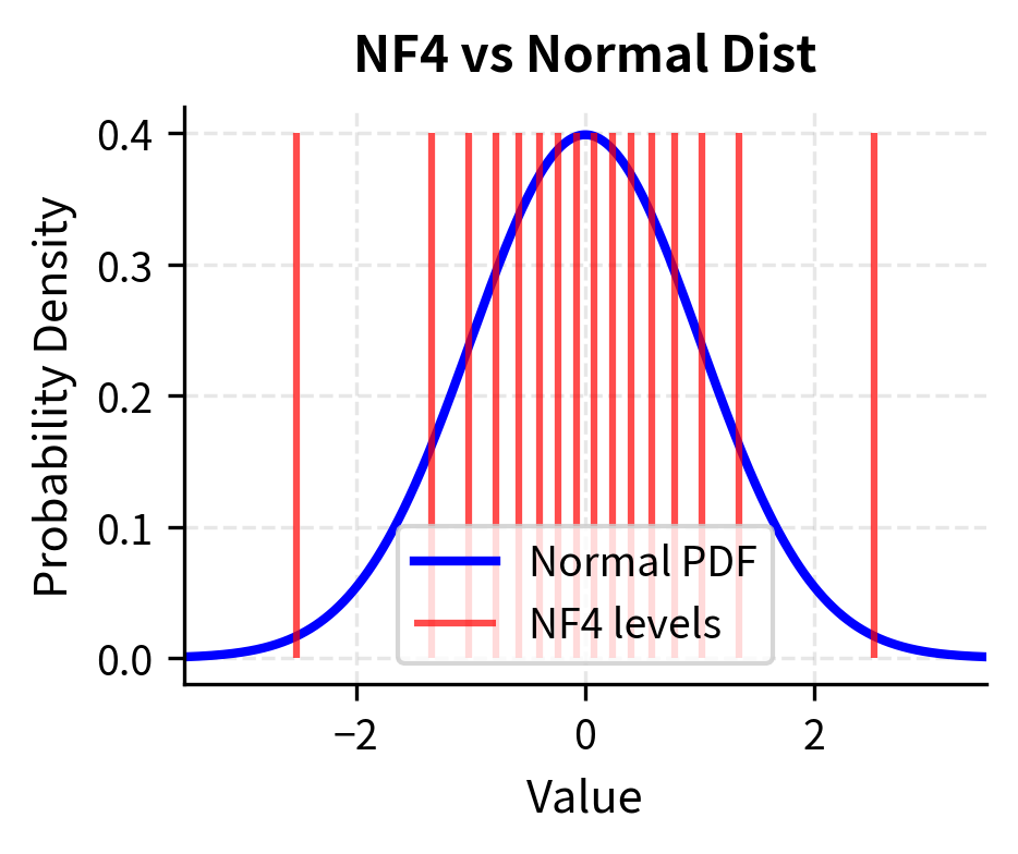
The visualization confirms that NF4 concentrates resolution where the data is, minimizing the expected error for Gaussian-distributed weights compared to the uniform grid of INT4. This distribution-aware approach to level placement is what makes NF4 particularly well-suited to neural network weight quantization, where approximate normality is a reasonable assumption for most layers.
FP4 (4-Bit Floating Point)
Another approach is to use a floating-point representation with 4 bits. This format attempts to bring the dynamic range advantages of floating-point to the extremely constrained 4-bit budget. FP4 typically uses:
- 1 sign bit, determining whether the value is positive or negative
- 2 exponent bits, controlling the magnitude or scale of the value
- 1 mantissa bit, providing a single binary digit of precision within each exponent range
This format has a dynamic range similar to floating point and can represent a wide range of values using the exponent. However, the single mantissa bit means each exponent range has only 2 possible values (the implicit leading 1 and either 0 or 1 in the mantissa position). This extreme coarseness limits the practical utility of FP4 for many applications.
FP4's values are concentrated near zero but with exponentially increasing gaps as values get larger, following the characteristic pattern of floating-point representations. This structure can be useful for weight distributions with heavy tails, where the ability to represent large outliers without sacrificing too much precision near zero is valuable. However, the extreme coarseness introduced by having only a single mantissa bit limits practical utility for most neural network applications, where the fine distinctions among small weights are often critically important.
Comparing 4-Bit Formats
Let's quantize the same weights using different 4-bit formats and compare the reconstruction error. This empirical comparison will reveal how format choice affects quantization quality for normally distributed data:
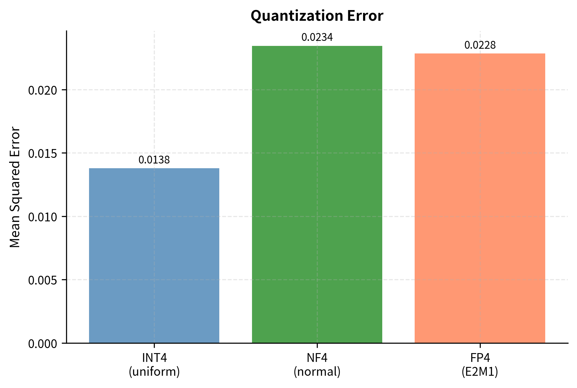
For normally distributed weights, NF4 provides lower quantization error than uniform INT4 because its levels are optimally placed for this distribution. This improvement is not coincidental but follows directly from the information-theoretic principles underlying NF4's design: by matching the quantization grid to the data distribution, we minimize expected reconstruction error.
Double Quantization
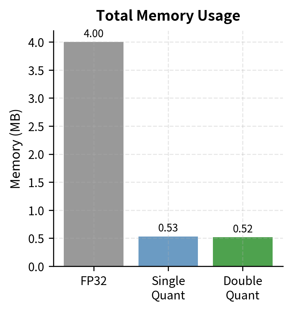
A technique called double quantization, also introduced with QLoRA, further reduces memory overhead by quantizing the scale factors themselves. This recursive application of quantization addresses a subtle but important issue with group-wise quantization. In standard group-wise quantization, we store one FP16 scale factor per group. With groups of 128, this adds 0.125 bits per weight (16 bits divided by 128 weights per group). While this overhead may seem modest, it becomes significant when the goal is to minimize memory footprint as aggressively as possible.
Double quantization applies a second round of quantization to these scale factors, treating them as a new quantization problem unto themselves:
- Collect all scale factors from the first quantization into a vector
- Group these scale factors together, typically in groups of 256
- Quantize the scale factors to FP8 or INT8 precision, which is coarser than FP16 but still accurate enough for scale factors
- Store a single FP32 scale factor per group of scale factors to enable reconstruction
The key insight enabling double quantization is that scale factors themselves exhibit predictable statistical properties. Within a neural network, scale factors for different groups tend to fall within a relatively narrow range, making them amenable to quantization without significant loss of information. The second-level scale factors (the "meta-scales") require only FP32 precision and are few in number, adding negligible overhead.
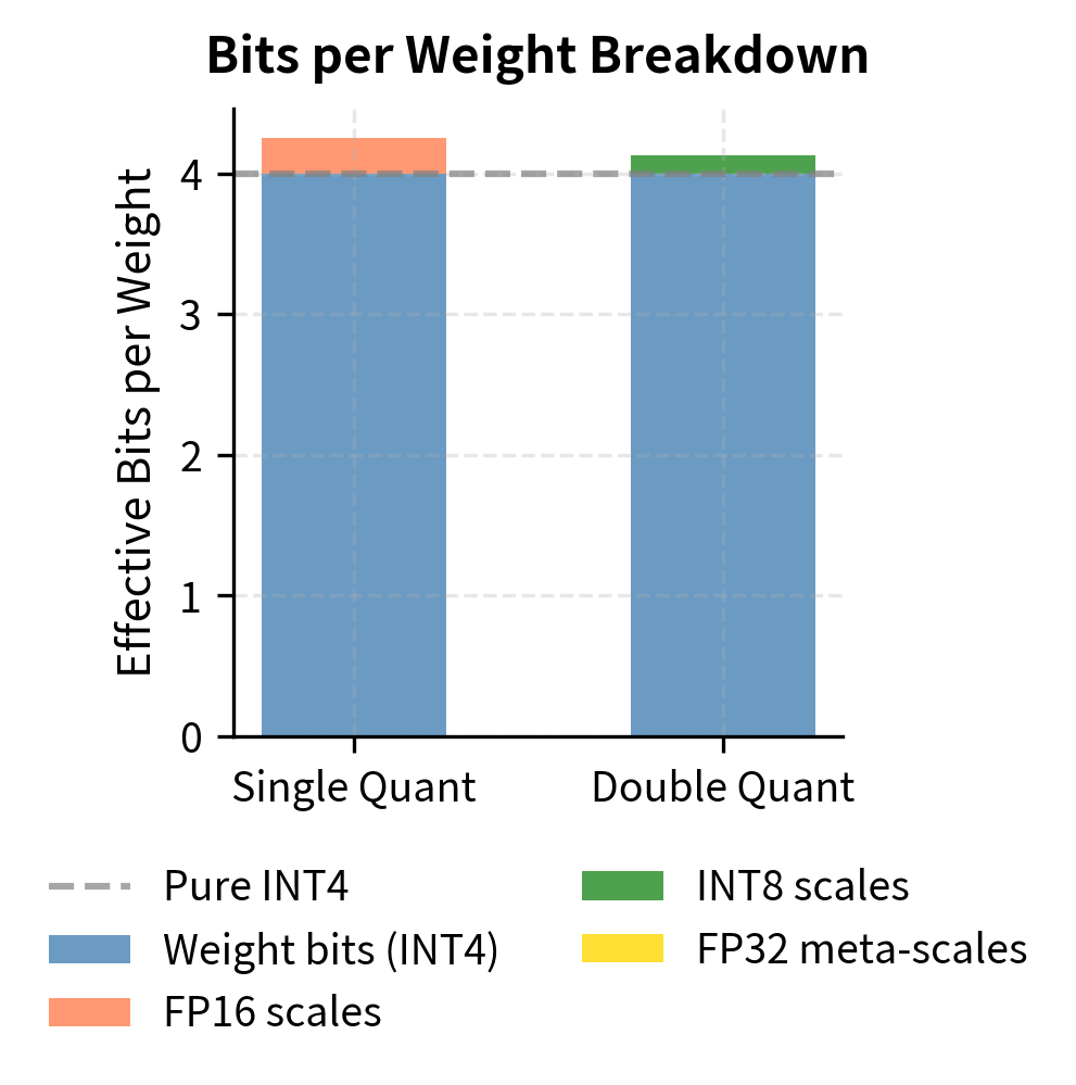
Double quantization reduces the overhead from scale factors, getting closer to true 4 bits per weight while maintaining the benefits of group-wise quantization. The additional complexity in the dequantization path (needing to reconstruct scales before reconstructing weights) is modest and well worth the memory savings for memory-constrained deployments.
Accuracy Trade-offs
How much does INT4 quantization affect model quality? The answer depends heavily on the model, task, and quantization technique used. Understanding these dependencies is crucial for making informed decisions about when and how to deploy 4-bit quantized models. Let's explore the key factors that determine INT4 success.
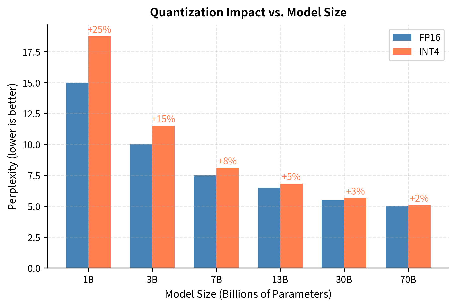
Model Size Matters
Larger models tolerate quantization better than smaller ones, a phenomenon that has been consistently observed across many model families and quantization methods. A 70B parameter model quantized to INT4 often performs comparably to its FP16 version, while a 7B model may show noticeable degradation. Larger models are more redundant and tolerate information loss from quantization better.
Larger models are more robust because they have more parameters to encode information. When quantization introduces errors into some of these parameters, the remaining parameters can compensate, maintaining the overall behavior of the network. Smaller models lack this redundancy: each parameter carries more information, and corrupting that information through quantization has proportionally larger effects.
Task Sensitivity
Different tasks have different sensitivity to quantization errors, and understanding this variation is important for deployment decisions. Tasks requiring precise numerical reasoning or factual recall tend to suffer more from quantization than tasks involving broader pattern recognition:
- More sensitive: Mathematical reasoning, code generation, factual question answering
- Less sensitive: Text summarization, sentiment analysis, general conversation
This sensitivity stems from how errors propagate through the model during different types of computation. For mathematical reasoning, a small error in intermediate calculations can compound into a wrong final answer. The model must maintain precise numerical relationships across many computation steps, and quantization errors can accumulate or interfere with these delicate calculations. For summarization, slightly imprecise representations still capture the overall meaning, and the model's task is more about recognizing patterns and relationships than performing exact computation.
Layer-Specific Quantization
Not all layers in a transformer contribute equally to model quality, and this observation has important implications for quantization strategy. Research has shown that certain layers are more sensitive to quantization errors than others:
- Attention projections (Q, K, V, and output projections): Often sensitive, especially in earlier layers, because they determine how information flows between positions in the sequence
- Feed-forward networks: Generally more robust to quantization, perhaps because they perform more local computations that are less affected by small perturbations
- Embedding layers: Very sensitive, often kept at higher precision, because they form the foundation upon which all subsequent computation builds
This observation leads to mixed-precision strategies where sensitive layers use INT8 while robust layers use INT4. Such strategies can achieve much of the memory savings of uniform INT4 quantization while retaining much of the accuracy of INT8 or even FP16 for critical operations:
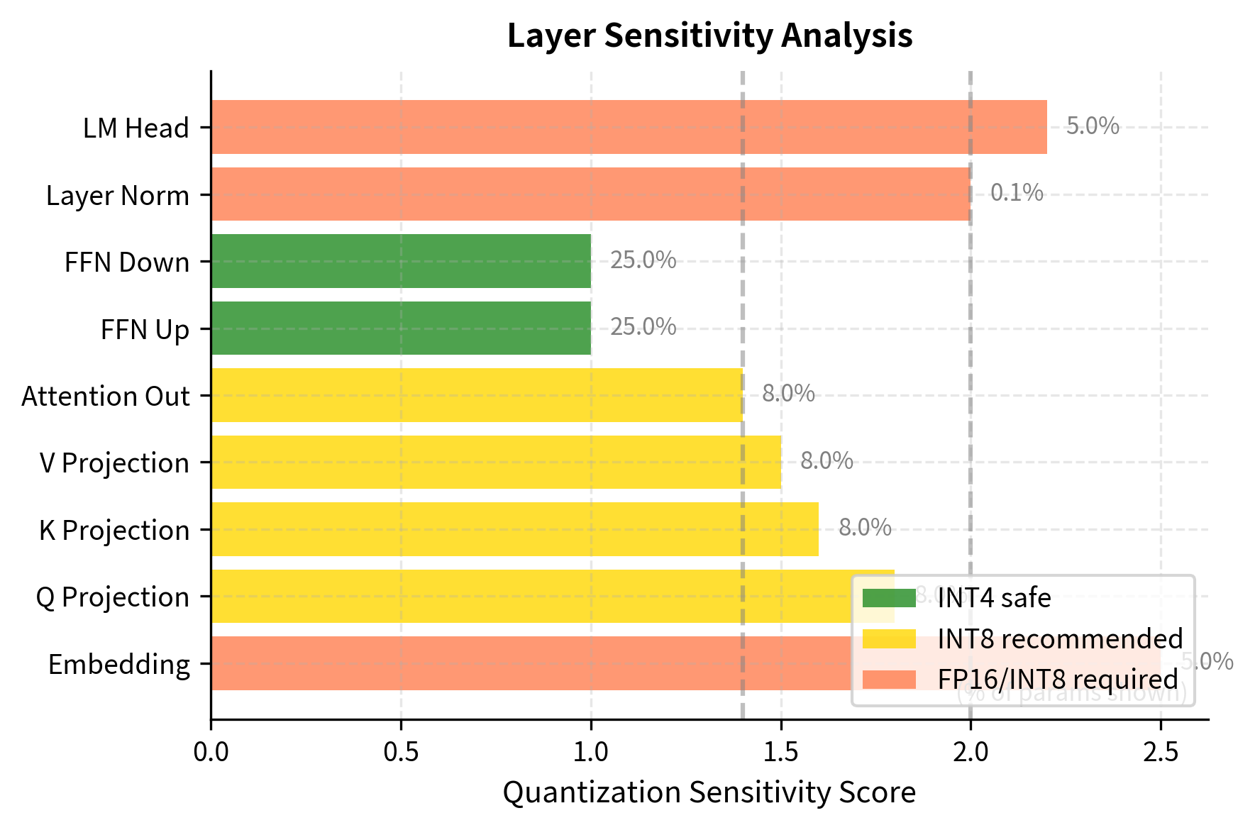
The results suggest a hybrid approach: retain high precision for embeddings and attention outputs, but aggressively quantize the feed-forward networks that contain the majority of parameters. Since FFN layers often account for roughly half of a transformer's parameters, quantizing them to INT4 while keeping other layers at INT8 can still provide substantial memory savings with minimal accuracy loss.
Practical Implementation with bitsandbytes
The bitsandbytes library provides efficient 4-bit quantization for PyTorch models. It implements NF4 quantization with group-wise scaling and double quantization, making it easy to load large models in 4-bit precision. The library handles format conversion, scale management, and dequantization during inference, providing a simple API.
Let's examine the memory savings:
This dramatic reduction allows a 7B model to fit comfortably within the 6GB or 8GB VRAM limits of many consumer GPUs, making powerful LLMs accessible on commodity hardware. What was previously possible only on expensive data center GPUs becomes achievable on hardware that many of you already own.
Limitations and Practical Considerations
INT4 quantization enables running large language models on consumer hardware, but it comes with important trade-offs that you must understand.
The most significant limitation is accuracy degradation on complex tasks. While INT4 models perform well on conversational AI and text generation, they often struggle with tasks requiring precise reasoning. Mathematical problem solving, multi-step logical inference, and tasks requiring exact factual recall show measurable degradation. For applications where accuracy is critical, INT8 or even FP16 may be necessary despite the higher memory cost.
Another practical concern is the computational overhead during inference. Although INT4 weights consume less memory, the dequantization step (converting INT4 back to FP16 for matrix multiplication) adds latency. Modern GPUs lack native INT4 compute support, so each forward pass must dequantize on the fly. This overhead is typically small relative to the overall forward pass, but it's not zero. Libraries like bitsandbytes and upcoming chapters on GPTQ and AWQ implement various optimizations to minimize this overhead.
Calibration requirements also vary between quantization methods. The simple symmetric quantization we implemented here doesn't require calibration data, but more sophisticated methods like GPTQ (covered in the next chapter) use calibration data to find optimal quantization parameters. The quality of calibration data affects the final model quality.
Finally, INT4 quantization is primarily a memory optimization, not a speed optimization. While reducing memory enables running larger models or larger batch sizes, the actual compute doesn't speed up proportionally because dequantization is required. For pure throughput optimization, other techniques like speculative decoding (covered later in this part) may be more effective.
Summary
INT4 quantization pushes the boundaries of model compression, reducing memory requirements to roughly 4.5 bits per weight (including scale factors). The key insights from this chapter are:
-
16 levels are not enough for naive uniform quantization. The limited representational capacity requires sophisticated techniques to maintain model quality.
-
Group-wise quantization is essential for INT4 success. By using separate scale factors for groups of 32-128 weights, outliers affect only their local group rather than the entire tensor.
-
NF4 format outperforms uniform INT4 for normally distributed weights by placing quantization levels to match the weight distribution. This format, introduced with QLoRA, has become the de facto standard for 4-bit inference.
-
Double quantization reduces the memory overhead from scale factors by quantizing the scales themselves, getting closer to true 4 bits per weight.
-
Model size and task complexity determine quantization tolerance. Larger models (30B+) typically maintain quality at INT4, while smaller models may need INT8 or mixed precision strategies.
The next chapter covers GPTQ, a calibration-based quantization method that uses second-order information to find optimal weight quantization, often achieving better accuracy than the simpler methods discussed here.
Quiz
Ready to test your understanding? Take this quick quiz to reinforce what you've learned about INT4 quantization techniques.

Comments