

Master INT8 weight quantization with absmax and smooth quantization techniques. Learn to solve the outlier problem in large language models.

This article is part of the free-to-read Language AI Handbook
Choose your expertise level to adjust how many terms are explained. Beginners see more tooltips, experts see fewer to maintain reading flow. Hover over underlined terms for instant definitions.
INT8 Quantization
In the previous chapter on weight quantization basics, we explored why representing neural network parameters with fewer bits can dramatically reduce memory requirements and accelerate inference. Now we dive into the most widely adopted quantization format: 8-bit integers (INT8). This precision point represents a sweet spot where memory savings are substantial (2x compression from FP16, 4x from FP32), specialized hardware acceleration is widely available, and accuracy degradation remains manageable for most applications.
INT8 quantization isn't just about storing numbers more compactly. Modern GPUs and specialized AI accelerators include dedicated INT8 matrix multiplication units that can achieve 2-4x higher throughput than their floating-point counterparts. NVIDIA's Tensor Cores, for example, perform INT8 operations at twice the rate of FP16 operations. This means that if we can quantize both weights and activations to INT8, we unlock not just memory savings but genuine compute speedup.
However, squeezing the continuous range of floating-point values into just 256 discrete integers introduces quantization error. Effective INT8 quantization minimizes this error while maximizing the benefits. We'll explore the mathematics of range mapping, the practical absmax quantization scheme, and the smooth quantization technique that makes INT8 viable even for large language models with problematic activation distributions.
The INT8 Representation Space
An 8-bit signed integer can represent values from -128 to 127, giving us 256 distinct values to work with. When we quantize a floating-point tensor, we're essentially creating a codebook that maps each of these 256 integers to a specific floating-point value. This mapping defines a correspondence between the rich, continuous space of floating-point numbers and a sparse, discrete set of representable points.
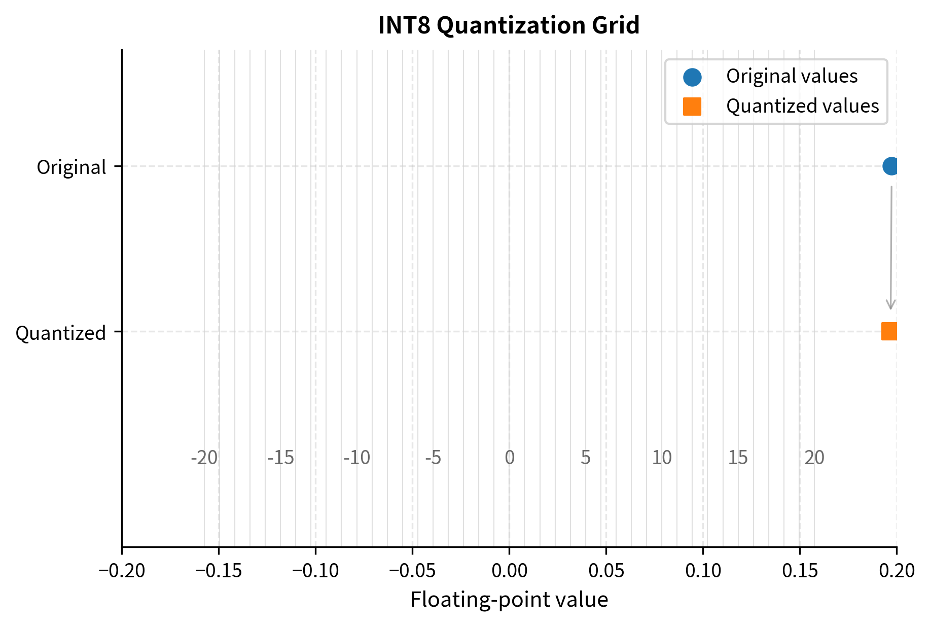
To understand this mapping intuitively, imagine you have a number line representing all possible floating-point values a weight might take. Quantization places 256 evenly-spaced "buckets" along this line, and every floating-point value must be assigned to its nearest bucket. The original value is then represented by that bucket's integer label, and reconstruction involves converting the label back to the bucket's center position. The spacing between these buckets, and where they are positioned along the number line, completely determines the quality of our approximation.
The set of representable values after quantization forms a uniform grid in the original floating-point space. The spacing between adjacent grid points is called the quantization step size or scale factor.
The fundamental challenge is choosing how to position this grid. Consider a weight tensor with values ranging from -0.5 to 1.2. We need to decide:
- What floating-point value should -128 represent?
- What floating-point value should 127 represent?
- How do we handle values outside our chosen range (clipping)?
These choices define our quantization scheme and directly impact the reconstruction error. A poorly chosen grid might waste many of its 256 integers representing values that never actually occur in the tensor, while cramming the values that do occur into too few buckets. The goal is to align our quantization grid as closely as possible with the actual distribution of values we need to represent.
Symmetric Quantization with Absmax
The simplest and most common approach is symmetric quantization, where we center the quantization grid at zero. The "absmax" method finds the maximum absolute value in the tensor and maps it to the largest representable integer. This approach derives its name from the key statistic it computes: the absolute maximum which determines the extent of our quantization range in both positive and negative directions simultaneously.
The intuition behind absmax quantization is straightforward. We want to ensure that no value in our tensor falls outside the representable range, which would force us to clip it and introduce potentially large errors. By finding the largest magnitude value in the tensor and designing our grid to just barely accommodate it, we guarantee that every original value can be represented without clipping. At the same time, we make the grid as fine as possible given this constraint, since using a larger range than necessary would waste precision.
Given a tensor with floating-point values, absmax quantization works as follows:
where:
- : the input floating-point tensor
- : the maximum absolute value in the input tensor (the "absmax")
- : the scale factor that determines the spacing of the quantization grid
- : the maximum representable value in a signed 8-bit integer
- : the resulting tensor of quantized 8-bit integers
Let's trace through this process step by step. First, we scan the entire tensor to find , the largest magnitude value regardless of sign. This becomes our reference point for setting the scale. Next, we compute the scale factor by dividing by 127, which tells us how much "floating-point distance" each integer step represents. Finally, we quantize each value by dividing it by the scale factor and rounding to the nearest integer. This rounding step is where the actual information loss occurs, as we snap each continuous value to its nearest discrete representation.
To recover an approximation of the original values, we simply multiply by the scale:
where:
- : the reconstructed floating-point tensor (an approximation of the original )
- : the scale factor used during quantization
- : the quantized integer tensor
The hat notation indicates this is a reconstruction, not the exact original values. The difference is the quantization error. This error arises because the rounding operation discards fractional information. When we divided by and rounded, we lost the remainder, and multiplying the rounded result back by cannot restore what was lost. The beauty of this scheme is that the error is bounded: no reconstructed value can differ from its original by more than half a scale step, or .
Why Symmetric Around Zero?
Centering the grid at zero has a crucial computational advantage: the integer zero maps exactly to floating-point zero. This property, which might seem like a minor mathematical nicety, turns out to have significant practical implications for neural network inference.
This matters because:
- Many neural network activations are zero (from ReLU, dropout, padding)
- Zero-valued weights don't contribute to computations
- Preserving exact zeros avoids accumulating unnecessary rounding errors
Consider what happens during a matrix multiplication when many elements are zero. If zero maps exactly to zero, these elements contribute nothing to the output, exactly as they should. But if zero were represented by some non-zero integer due to an offset, every "zero" element would actually contribute a small spurious value to the computation. Over millions of operations, these spurious contributions could accumulate into meaningful errors.
Symmetric quantization also simplifies the math during matrix multiplication. When computing with quantized values, we only need to track scale factors, not additional offset terms. This simplification translates directly into faster inference, since the dequantization step requires only a single multiplication rather than a multiplication followed by an addition.
The Clipping Trade-off
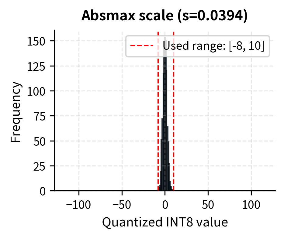
Absmax quantization clips all values to the range . If is dominated by a few outlier values, the quantization grid becomes coarse for the majority of values. This creates a fundamental tension in quantization design: we want to accommodate outliers to avoid clipping errors, but we also want a fine grid to minimize rounding errors for typical values.
Consider a tensor where 99% of values lie between -0.1 and 0.1, but one outlier is 5.0. Using absmax:
This scale means values around 0.1 get quantized to just . The reconstruction is , introducing significant relative error for these common values. To understand the magnitude of this problem, note that a typical value of 0.1 experiences an 18% relative error, while the outlier value of 5.0 would be reconstructed nearly perfectly. We have sacrificed precision where it matters most, on the bulk of our values, to perfectly preserve a single outlier.
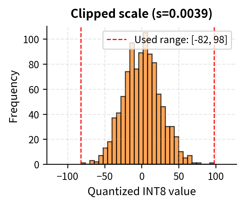
One solution is to clip outliers: choose smaller than the true maximum, accepting that extreme values will be clipped. This trades outlier accuracy for better precision on the bulk of values. For example, if we set instead of 5.0, our scale becomes , and a value of 0.1 now quantizes to integer 25 with reconstruction , a much smaller relative error. The outlier would be clipped to 127, reconstructing to 0.5 instead of 5.0, but this might be an acceptable trade-off depending on the model's sensitivity.
Finding the optimal clipping threshold is the basis for calibration-based quantization methods. These methods analyze the value distribution across representative data to find the clipping point that minimizes total reconstruction error, balancing the clipping errors from outliers against the rounding errors for typical values.
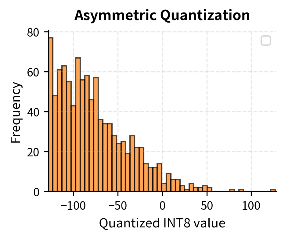
Asymmetric Quantization
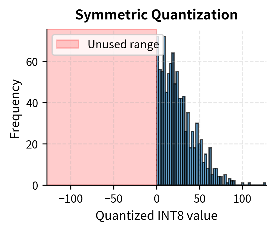
When tensor values aren't centered around zero, symmetric quantization wastes representable range. ReLU activations, for example, are always non-negative. Mapping the range symmetrically would waste half our integers representing negative values that never occur. This inefficiency becomes severe when the actual data distribution is heavily skewed or shifted away from zero.
Asymmetric quantization introduces a zero-point offset to shift the quantization range:
where:
- : the input floating-point tensor
- : the scale factor, computed from the full range of values
- : the number of intervals in an 8-bit range ()
- : the zero-point integer that shifts the grid to align with the data distribution
- : the resulting quantized tensor
The key difference from symmetric quantization lies in how we compute the scale and the introduction of the zero-point. Instead of basing the scale on the maximum absolute value, we use the full range from minimum to maximum, ensuring all 256 integers can potentially be used. The zero-point is an integer that shifts the quantization grid so that the minimum value maps to -128 and the maximum to 127. This shift allows us to "slide" our quantization grid along the number line to wherever the actual data lies.
Dequantization becomes:
where:
- : the reconstructed floating-point values
- : the scale factor
- : the quantized integer values
- : the zero-point offset, which is subtracted before scaling
While asymmetric quantization can represent arbitrary ranges more efficiently, it complicates the math during inference. Matrix multiplications now involve additional terms from the zero-point offsets. When we expand the matrix multiplication with asymmetric quantization, cross-terms involving the zero-points appear, requiring additional computation and memory access. For weights, which are typically centered around zero due to common initialization and regularization practices, symmetric quantization remains the standard choice. The computational overhead of asymmetric quantization is generally reserved for activations where the efficiency gains from better range utilization outweigh the additional complexity.
Per-Tensor vs Per-Channel Quantization
The granularity at which we compute scale factors significantly impacts quantization quality. This design choice represents a trade-off between simplicity and accuracy, with different granularities being appropriate for different situations.
Per-tensor quantization uses a single scale factor for an entire weight matrix or activation tensor. This is simple and introduces minimal overhead, but a single outlier anywhere in the tensor degrades precision everywhere. Imagine a weight matrix where one row has unusually large values: that single row would force a large scale factor that reduces precision for all other rows.
Per-channel quantization computes separate scale factors for each output channel of a weight matrix. For a linear layer with weight matrix , we compute different scale factors, one for each column (corresponding to each output channel):
where:
- : the scale factor for the -th output channel (column)
- : the vector of weights corresponding to the -th output channel
- : the maximum absolute value in that channel's weights
- : the maximum value for a signed 8-bit integer
This allows each output channel to use its full INT8 range, accommodating the fact that different channels often have different magnitude distributions. Consider why this happens: during training, different output features may learn patterns of varying intensity, leading some channels to develop larger weight magnitudes than others. Per-channel quantization respects these differences by giving each channel its own appropriately-sized quantization grid.
The overhead is storing scale factors instead of one, which is negligible compared to the weight tensor itself. For a layer with 4096 output channels and 4096 input features, we store 4096 scale factors (one per channel) versus over 16 million quantized weights. The scale factors add less than 0.1% to the storage requirements while potentially dramatically improving accuracy.
Per-channel quantization for weights combined with per-tensor quantization for activations has emerged as the standard approach, offering good accuracy with manageable complexity. The asymmetry makes sense: weights are static and can be analyzed offline to compute optimal per-channel scales, while activations vary with each input and would require expensive runtime scale computation for per-channel treatment.
The Outlier Problem in Large Language Models
As language models scale to billions of parameters, a problematic pattern emerges: certain activation dimensions develop extreme outlier values. Research has shown that in models like OPT-175B and BLOOM-176B, a small number of hidden dimensions (sometimes called "massive activations" or "emergent features") can have values 10-100x larger than typical activations. This phenomenon was not anticipated by early quantization research and poses a significant challenge to naive INT8 approaches.
The emergence of these outliers appears to be linked to how transformers process information at scale. Certain hidden dimensions seem to serve as "highways" for important information, developing consistently large activation magnitudes across many inputs. These are not random fluctuations but systematic features of the model's learned representations. While we are still working to fully understand why this happens, the practical implication is clear: any quantization strategy for large language models must account for these outliers.
These outliers create a severe quantization challenge. Consider a hidden state where 99.9% of values lie in , but dimension 1847 consistently produces values around 50. Per-tensor absmax quantization would set , meaning values of magnitude 1 quantize to just 2-3 integers. The reconstruction error for these common values becomes unacceptable. A value of 0.5, which might be crucial for the model's computation, would quantize to either 1 or 2, introducing errors of up to 20% in its representation.
The naive solutions all have drawbacks:
- Clipping outliers: Destroys important model information encoded in those dimensions
- Per-channel activation quantization: Requires computing new scale factors for every token, adding latency
- Mixed precision: Keeping outlier channels in FP16 complicates kernels and reduces throughput
Each of these approaches involves either losing accuracy, losing speed, or adding significant implementation complexity. What we needed was a technique that could tame the outlier problem without sacrificing the efficiency benefits of uniform INT8 quantization.
Smooth quantization offers a practical mathematical solution.
Smooth Quantization
The key insight behind smooth quantization is that while activations are hard to quantize (dynamic, contain outliers), weights are easy to quantize (static, relatively uniform). We can mathematically migrate the quantization difficulty from activations to weights through a channel-wise scaling transformation. This insight transforms the problem from one that seems intractable to one that has a clean solution.
The intuition is straightforward: if one matrix is "spiky" with outliers and another is "smooth" and well-behaved, we can transfer some of the spikiness from the first to the second. As long as we do this in a mathematically consistent way that preserves the final computation, we haven't changed the model's behavior, only redistributed the quantization difficulty.
The Mathematical Equivalence
Consider a linear layer computing , where is the activation input and is the weight matrix. We introduce a diagonal matrix with positive scaling factors:
where:
- : the output of the linear layer
- : the input activation tensor
- : the weight matrix
- : a diagonal smoothing matrix containing scaling factors for each input dimension
- : the smoothed activation matrix ()
- : the adjusted weight matrix ()
This transformation is mathematically exact since . We haven't changed the computation, just how we factor it. The key mathematical property we exploit is that multiplying by a matrix and then its inverse produces the identity, so inserting between and changes nothing about the final result. We are free to group these factors however we like, and we choose to group with the activations and with the weights.
The transformation affects the data as follows:
- Smoothed activations: divides each column of by
- Adjusted weights: multiplies each row of by
If channel has outlier activations, we choose a large . This shrinks the activations (making them easier to quantize) while enlarging the corresponding weights (which are already easy to quantize). We're transferring the outlier problem to a domain where it's more manageable. Since the weights typically have plenty of "headroom" before they become difficult to quantize, they can absorb the increased magnitude from the outlier channels without significant accuracy loss.
Choosing the Smoothing Factors
How do we pick the values? If we make too large, we might shrink the activations so much that we lose precision in other ways, or we might inflate the weights to the point where they become hard to quantize. The optimal choice balances these competing concerns.
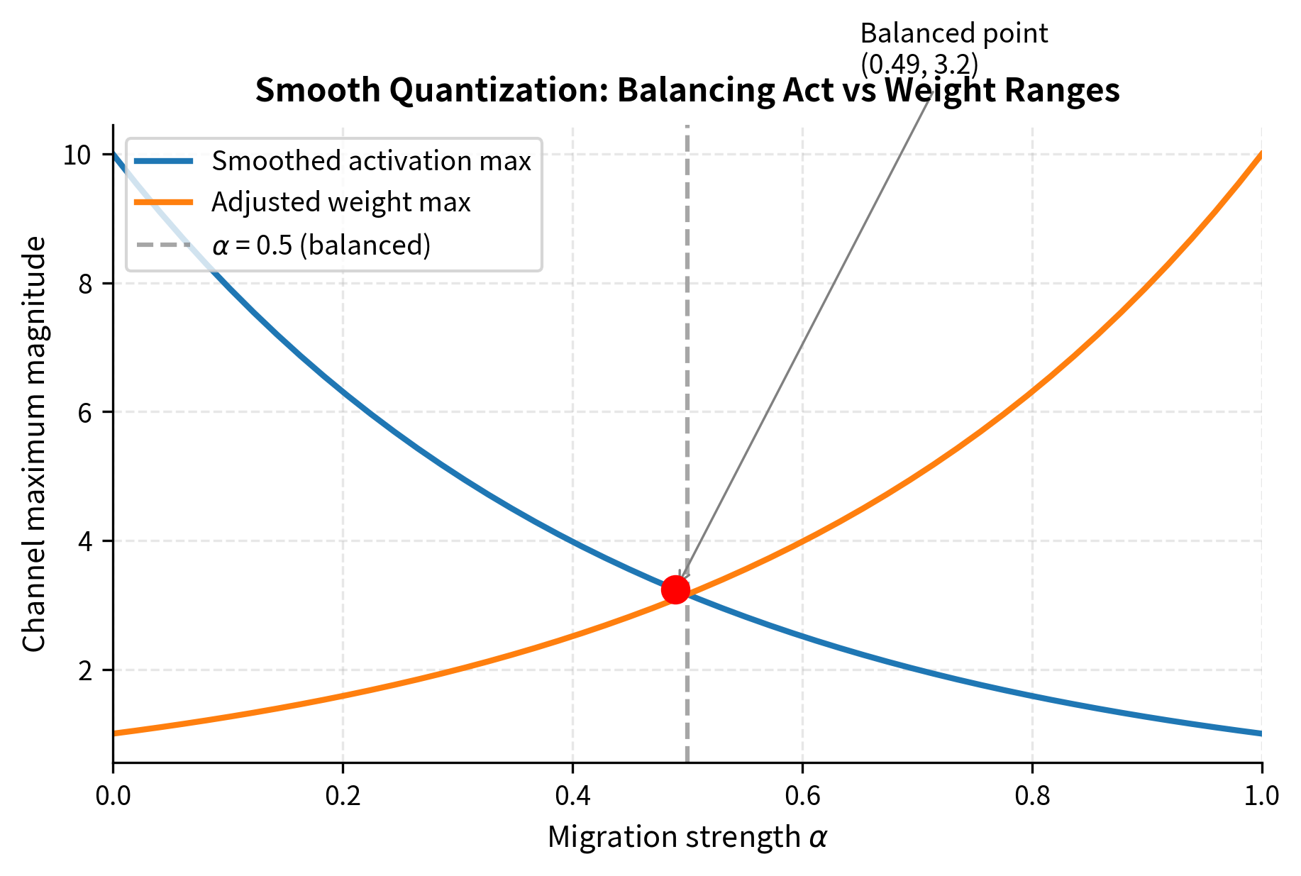
The SmoothQuant paper proposes balancing the quantization difficulty between activations and weights using a migration strength parameter :
where:
- : the smoothing factor for the -th input channel
- : the maximum absolute value in the -th column of activations (across the calibration set)
- : the maximum absolute value in the -th row of weights (corresponding to the -th input feature)
- : the migration strength hyperparameter controlling how much difficulty is shifted from activations to weights
This formula balances two competing goals:
- When : , fully smoothing activations but potentially making weights hard to quantize
- When : , leaving activations unchanged
- When : Balances the maximum values of both smoothed activations and adjusted weights
To understand this formula intuitively, consider what happens at . The smoothing factor becomes the geometric mean of the activation maximum and the reciprocal of the weight maximum. This choice ensures that after transformation, the maximum activation and maximum weight for each channel have roughly equal magnitude, spreading the quantization difficulty evenly between the two matrices.
In practice, works well for most models, achieving roughly equal quantization ranges for both activations and weights after smoothing. However, some models may benefit from different values. Models with particularly severe activation outliers might use to more aggressively smooth the activations, while models with already-difficult-to-quantize weights might use to avoid making the weights worse.
Offline Computation
A critical practical advantage of smooth quantization is that the transformation can be computed offline during a calibration phase:
- Run a small calibration dataset through the model to collect activation statistics
- Compute for each channel using these statistics
- Calculate smoothing factors for each layer
- Apply the weight transformation and store the modified weights
- Fuse into the preceding layer's weights or normalization parameters
Step 5 is crucial: rather than explicitly dividing activations by at runtime, we absorb this division into the bias of the previous layer or the scale/shift parameters of the preceding LayerNorm. This means inference has zero additional cost compared to standard quantized inference.
The fusion works because transformer architectures typically have a LayerNorm immediately before each linear layer. LayerNorm applies a learned scale and shift to each channel, and we can simply incorporate the smoothing factor into these existing parameters. If the original LayerNorm scale for channel was and shift was , we replace them with and . The activations coming out of the modified LayerNorm are already "smoothed," and we never need to perform the division at runtime.
Quantized Matrix Multiplication
Understanding how quantized operations execute helps clarify why INT8 provides speedup. When both weights and activations are in INT8, the matrix multiplication proceeds as:
where:
- : the intermediate result matrix stored in 32-bit integers
- : the quantized input activations (8-bit integers)
- : the quantized weights (8-bit integers)
The integer multiplication produces INT32 results to avoid overflow from accumulating many INT8×INT8 products. To understand why this is necessary, consider that each INT8×INT8 multiplication produces a result up to , which still fits in INT16. However, a matrix multiplication accumulates thousands or millions of such products, and these sums can easily exceed the INT16 range. INT32 provides enough headroom to accumulate the typical number of products found in neural network layers without overflow.
We then convert back to floating-point and apply scale factors:
where:
- : the final floating-point output
- : the quantization scale factor for the activations
- : the quantization scale factor for the weights (scalar or vector depending on quantization granularity)
- : the integer output from the matrix multiplication, converted to float before scaling
The scale factors and are the quantization scales for activations and weights respectively. Since scale factors are scalar (or per-channel), this final rescaling is cheap compared to the matrix multiplication itself. The computational cost of the rescaling step is for an output matrix of size , while the matrix multiplication itself is for matrices of appropriate dimensions. Since is typically large (thousands of features), the rescaling overhead is negligible.
Hardware INT8 units execute this pattern efficiently because:
- INT8 multiply-accumulate operations are simpler than floating-point
- Smaller operands allow higher parallelism in the same silicon area
- Memory bandwidth is halved, reducing the primary bottleneck for large models
The silicon area argument is particularly important. A floating-point multiplier requires circuits for handling sign bits, exponents, and mantissas, with additional logic for normalization and special cases. An integer multiplier needs only straightforward binary multiplication. This simplicity means that in the same chip area, hardware designers can fit more INT8 units than floating-point units, enabling higher parallelism. Combined with the reduced memory bandwidth from smaller data types, INT8 quantization provides compounding benefits that translate to real-world speedups.
Implementation
Let's implement INT8 quantization from scratch to solidify these concepts.
Absmax Quantization
We'll start with the fundamental absmax quantization and dequantization operations:
Let's test this on a simple tensor:
The maximum error is bounded by half the quantization step size (), as values are rounded to the nearest integer. For this tensor with a scale around 0.01, our maximum possible error is about 0.005.
Analyzing Quantization Error
Let's visualize how quantization error varies across different value ranges:
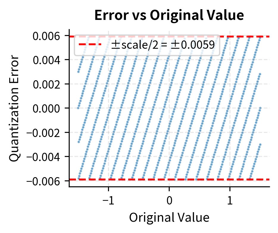
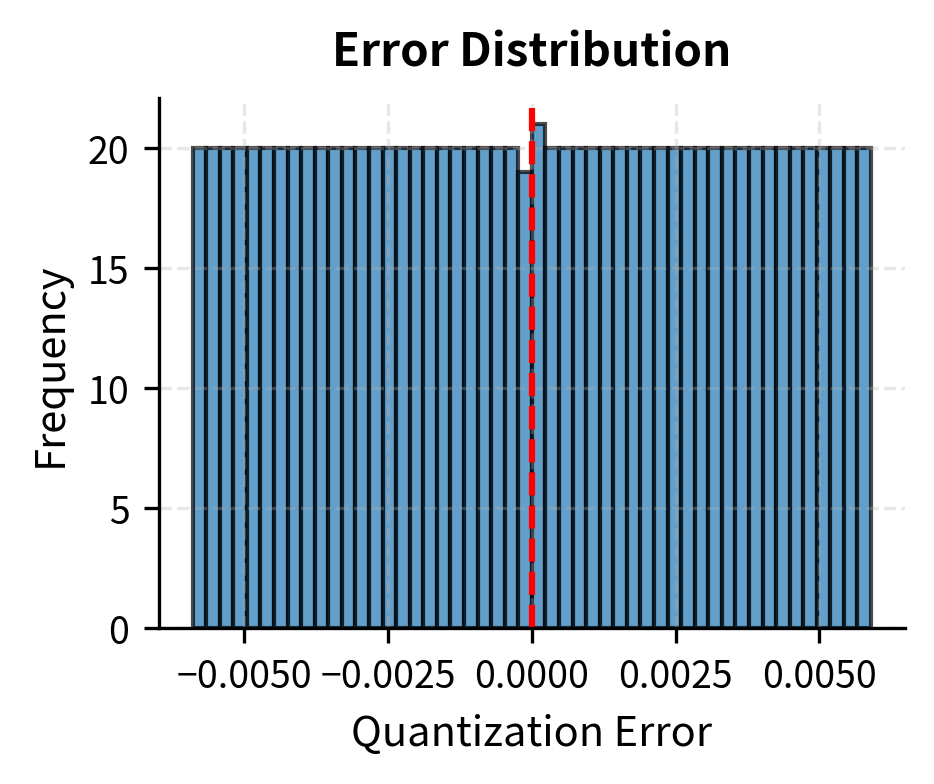
The error follows a uniform distribution between and , which is exactly what we expect from rounding to the nearest integer on a uniform grid.
Per-Channel Quantization
Now let's implement per-channel quantization for weight matrices:
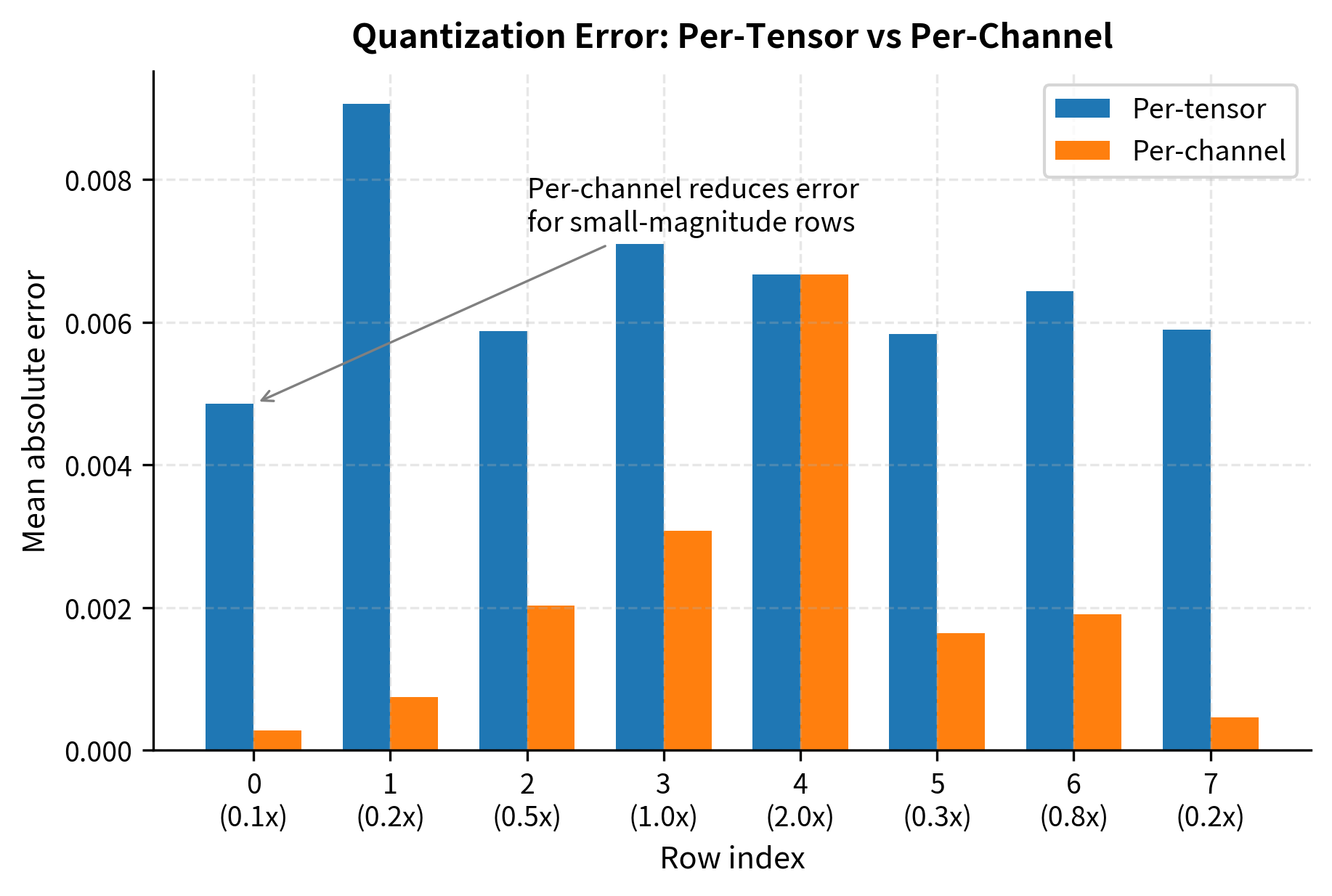
Let's compare per-tensor vs per-channel quantization on a weight matrix with varying row magnitudes:
Per-channel quantization achieves substantially lower error, especially for rows with small magnitudes. The per-tensor approach is forced to use a scale dictated by the largest row, wasting precision for smaller rows.
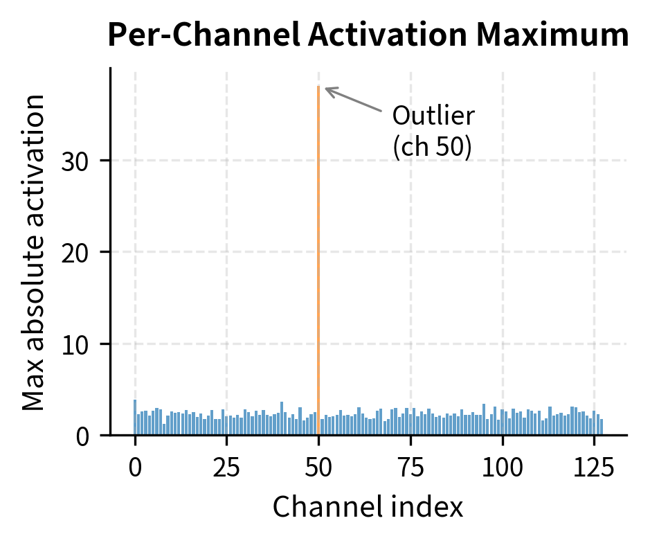
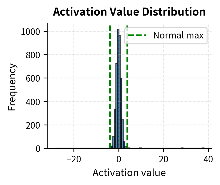
Demonstrating the Outlier Problem
Let's simulate the outlier pattern seen in large language models:
The outlier channel forces a large scale factor, causing severe relative error for normal channels. This is exactly the problem that smooth quantization solves.
Implementing Smooth Quantization
Now let's implement the smooth quantization transformation:
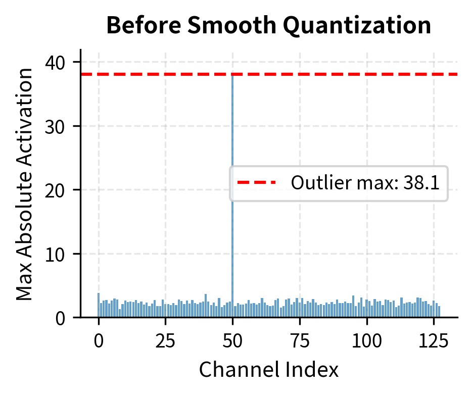
Let's apply smooth quantization to our outlier problem:
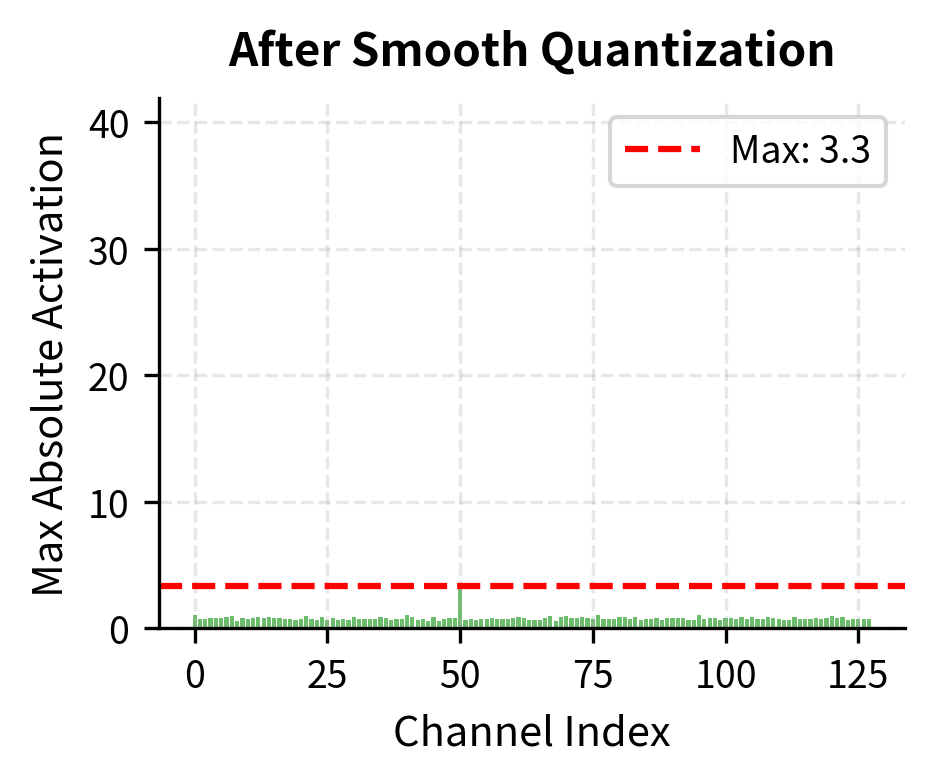
Smooth quantization dramatically reduces the activation range ratio, making per-tensor quantization much more effective. The error for normal channels drops significantly because they're no longer penalized by the outlier's presence.
Visualizing the Smoothing Effect
End-to-End Quantized Linear Layer
Let's put everything together into a complete quantized linear layer:
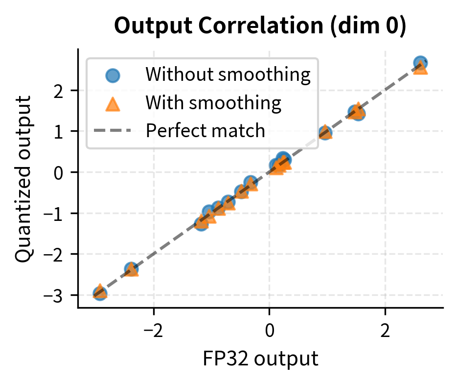
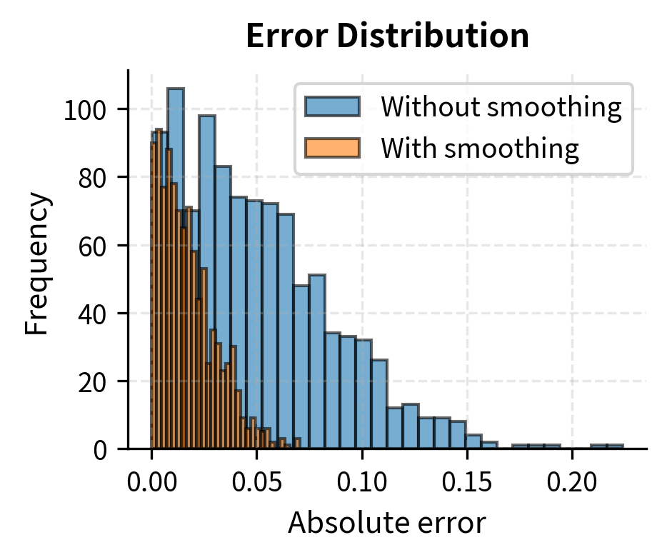
Now let's compare the quantized layer against full precision:
Smooth quantization reduces both maximum and mean error, making INT8 quantization viable even with outlier activations.
Key Parameters
The key parameters for the INT8 quantization implementation are:
- alpha: The migration strength in smooth quantization (typically 0.5). Controls how much quantization difficulty is shifted from activations to weights.
- scale: The step size of the quantization grid. Determined by the maximum absolute value (absmax) in the tensor or channel.
- smooth_scales: The channel-wise scaling factors derived from calibration data to balance activation and weight magnitudes.
INT8 Accuracy in Practice
The accuracy impact of INT8 quantization varies significantly based on model architecture, size, and task. Here's what research and practice have shown:
Models under 1B parameters typically quantize to INT8 with minimal degradation (less than 1% accuracy loss on benchmarks). The weight distributions are well-behaved, and activation outliers are rare.
Models from 1B to 10B parameters show increasing sensitivity. Without techniques like smooth quantization, accuracy can degrade 2-5% on certain tasks. Perplexity increases are noticeable but often acceptable for deployment.
Models above 10B parameters exhibit the emergent outlier features that make naive INT8 quantization fail. Smooth quantization or similar techniques become essential, restoring accuracy to near-FP16 levels.
Task sensitivity also matters:
- Simple classification tasks are robust to quantization
- Open-ended generation shows more degradation as errors compound
- Mathematical reasoning and code generation are particularly sensitive
The key insight is that INT8 quantization is not a one-size-fits-all solution. Calibration data choice, quantization granularity, and outlier handling all need tuning for optimal results.
Limitations and Practical Considerations
INT8 quantization represents a practical and widely-deployed optimization, but it comes with important limitations that you should understand.
The most fundamental limitation is that some model information is permanently lost during quantization. While smooth quantization and careful calibration minimize this loss, they cannot eliminate it entirely. For safety-critical applications or tasks requiring the highest possible accuracy, the small degradation from INT8 may be unacceptable. This is why many production systems maintain FP16 or FP32 models for evaluation and fine-tuning while deploying INT8 for inference.
Calibration data sensitivity presents another challenge. Smooth quantization computes channel-wise statistics from a calibration dataset, and if this data doesn't represent the actual deployment distribution, the smoothing factors may be suboptimal. A model calibrated on English text may perform poorly when quantized for code completion or multilingual inputs. You must ensure calibration data matches deployment conditions.
Hardware support, while widespread, is not universal. INT8 acceleration requires specific hardware features (like NVIDIA's Tensor Cores or ARM's NEON instructions), and the speedup varies by platform. On CPUs without INT8 vectorization, quantized inference may actually be slower than FP32 due to the quantization/dequantization overhead. Always benchmark on target hardware before committing to a quantization strategy.
Finally, INT8 may not provide sufficient compression for edge deployment. With 8 bits per weight, a 7B parameter model still requires 7GB of storage. For mobile or embedded applications, the more aggressive INT4 quantization techniques we'll explore in the next chapter become necessary, accepting greater accuracy trade-offs for smaller model sizes.
Summary
INT8 quantization provides a practical path to halving model memory and accelerating inference through hardware INT8 units. The key concepts are:
- Absmax quantization maps floating-point values to INT8 using a single scale factor, centering the quantization grid at zero
- Per-channel quantization applies separate scales to each output channel, reducing error when channels have different magnitude distributions
- The outlier problem emerges in large language models where a few activation dimensions have values 10-100x larger than typical, making per-tensor quantization fail
- Smooth quantization solves this by migrating quantization difficulty from activations to weights through a mathematically equivalent transformation
- The smoothing factor balances activation and weight ranges, computed offline from calibration data and fused into preceding layers
INT8 quantization with smooth quantization achieves near-FP16 accuracy on models up to hundreds of billions of parameters while providing 2x memory reduction and significant throughput improvements on compatible hardware. For even more aggressive compression, the upcoming chapters on INT4 quantization, GPTQ, and AWQ explore techniques that push quantization to just 4 bits per weight.
Quiz
Ready to test your understanding? Take this quick quiz to reinforce what you've learned about INT8 quantization techniques.

Comments