

Learn how weight quantization maps floating-point values to integers, reducing LLM memory by 4x. Covers scale, zero-point, symmetric vs asymmetric schemes.

This article is part of the free-to-read Language AI Handbook
Choose your expertise level to adjust how many terms are explained. Beginners see more tooltips, experts see fewer to maintain reading flow. Hover over underlined terms for instant definitions.
Weight Quantization Basics
Large language models are memory hogs. A 7 billion parameter model stored in 16-bit precision requires 14 GB just for the weights, and larger models scale proportionally: 70B parameters means 140 GB. As we discussed in the KV Cache chapters, memory bandwidth often bottlenecks LLM inference more than raw compute. Every forward pass must load billions of parameters from memory into the GPU's compute units, and this data movement dominates inference latency.
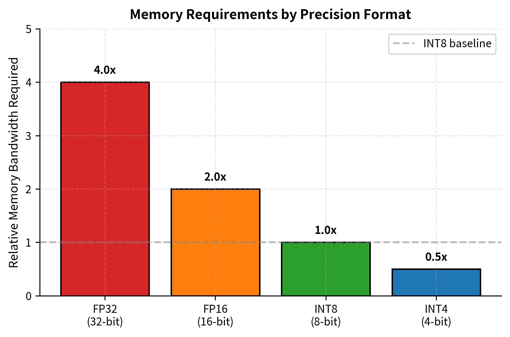
Quantization provides a direct solution: represent model weights using fewer bits. Instead of 16 or 32 bits per parameter, we can use 8, 4, or even fewer bits. This shrinks memory footprint, reduces bandwidth requirements, and often enables hardware-accelerated integer arithmetic that runs faster than floating-point operations. A 4-bit quantized 70B model fits in 35 GB, making it deployable on consumer hardware that couldn't touch the original.
But quantization isn't free. Cramming continuous values into discrete bins inevitably loses information. The goal of quantization is minimizing this loss while maximizing compression. This chapter covers the fundamental concepts: how quantization maps floats to integers, the different schemes for choosing that mapping, and how calibration finds optimal parameters for a given model.
Why Memory Bandwidth Limits Inference
Before diving into quantization mechanics, let's understand why memory dominates LLM inference costs. Modern GPUs have enormous compute throughput. An NVIDIA A100 delivers 312 teraflops of FP16 compute but only 2 TB/s of memory bandwidth. For each byte loaded from memory, the GPU can perform roughly 156 floating-point operations.
During autoregressive generation, each token requires loading essentially all model weights once. A single matrix multiplication of shape (where is the model dimension and is the feed-forward dimension) loads parameters but performs only floating-point operations. With a batch size of 1, this gives an arithmetic intensity of just 2 FLOPs per loaded element. GPUs capable of 156 FLOPs per byte sit idle waiting for data.
Quantization directly attacks this bottleneck. Loading 4-bit weights instead of 16-bit weights moves 4 times less data across the memory bus. Even if dequantization adds some computational overhead, the memory savings dominate for small-batch inference. This explains why quantization has become essential for efficient LLM deployment.
The Quantization Mapping
The process of mapping values from a continuous (or high-precision) representation to a discrete (or lower-precision) representation. In neural network contexts, this typically means converting 32-bit or 16-bit floating-point numbers to 8-bit or smaller integers.
At its core, quantization addresses a fundamental tension between precision and efficiency. Neural networks learn weights as floating-point numbers, which can represent an enormous range of values with fine granularity. However, this precision comes at a cost: each 32-bit float consumes four bytes of memory, and operations on floating-point numbers require specialized hardware circuits. The key insight behind quantization is that neural networks are remarkably robust to small perturbations in their weights. We don't need exact values; we need values that are close enough to preserve the network's learned behavior.
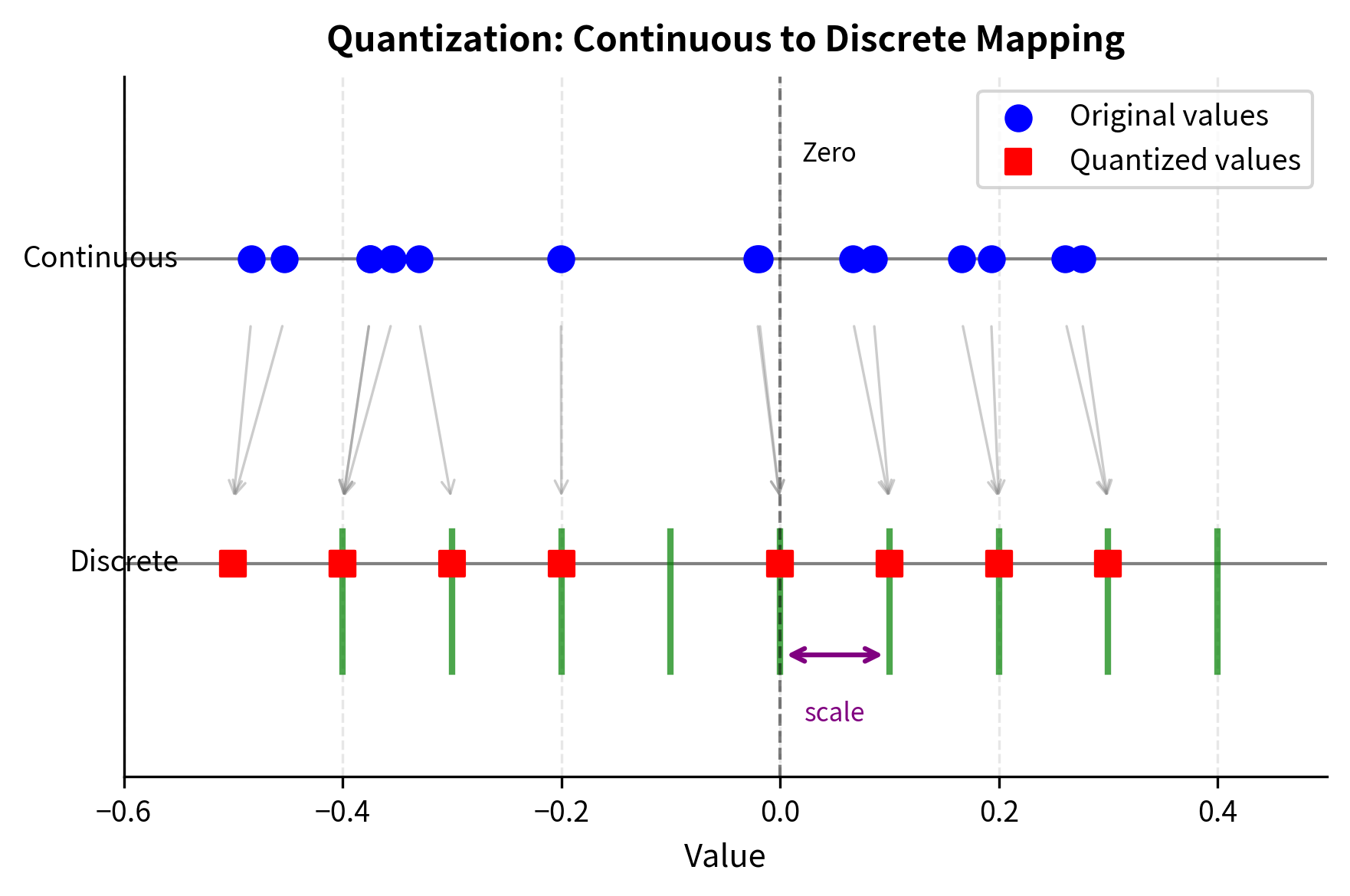
Consider a weight tensor with values ranging from to . We want to represent these using 8-bit signed integers, which can hold values from to . The mapping must preserve the relative relationships between values while fitting them into our target range. Think of this as creating a ruler where each tick mark represents one integer value, and we need to position values from the original continuous number line onto the nearest tick mark.
The standard affine quantization formula maps a real value to a quantized integer :
where:
- : the quantized integer value
- : the input real value (floating-point)
- : the scale factor, determining the step size of the quantization grid
- : the zero-point, an integer value to which real zero is mapped
- : the rounding operation (typically to the nearest integer)
This formula captures the essence of what quantization does. First, we divide the real value by the scale, which converts from real units to "quantization units." The scale determines how much of the real number line each integer step represents. If the scale is 0.01, then adjacent integers represent values that differ by 0.01 in the original space. After scaling, we round to the nearest integer because integers cannot represent fractional values. Finally, we add the zero-point, which shifts the entire mapping so that real zero lands on a particular integer value rather than necessarily on integer zero.
The zero-point serves an important purpose: it allows the quantized representation to efficiently use the available integer range even when the original values are not centered at zero. If all your weights happen to be positive, you would waste half the signed integer range without a zero-point adjustment.
To recover the original value (approximately), we apply the inverse dequantization operation:
where:
- : the reconstructed real value (approximation of the original )
- : the scale factor
- : the quantized integer
- : the zero-point
The dequantization formula simply reverses the quantization process. We first subtract the zero-point to undo the shift, then multiply by the scale to convert back from integer units to real units. Notice the hat notation on , which signals that this is an approximation rather than the exact original value. The reconstructed value won't exactly equal due to rounding, and this difference constitutes quantization error. Our goal is choosing and to minimize this error across the tensor.
Determining Scale and Zero-Point
With the quantization formula established, we now face a practical question: how do we choose the scale and zero-point? These parameters must be selected carefully because they determine both the range of representable values and the precision within that range. The intuition is straightforward: we want to map the full range of actual tensor values onto the full range of available integers, using every bit of precision the integer format provides.
We derive the quantization parameters by establishing a linear mapping where the real minimum maps to the integer minimum and maps to . This ensures that the smallest and largest values in our tensor precisely hit the boundaries of the integer range, leaving no representable integers unused.
where:
- : the minimum and maximum values in the real (floating-point) tensor
- : the minimum and maximum values in the target integer range (e.g., -128 and 127)
- : the scale factor to be determined
- : the zero-point to be determined
These two equations represent the boundary conditions of our linear mapping. The first equation says that when we dequantize the minimum integer value, we should recover the minimum real value. The second says the same for the maximum. Together, they give us two equations with two unknowns, which we can solve algebraically.
Subtracting the first equation from the second eliminates , which is the key insight that makes this system tractable:
Solving for yields the scale factor:
where:
- : the scale factor representing the step size (real value per integer increment)
- : the total range of the continuous values
- : the total number of discrete steps available
This formula has a straightforward interpretation: the scale is simply the ratio of the real range to the integer range. If your real values span 1.0 units and you have 256 integers available, each integer step represents real units. The scale tells you exactly how much precision you have: smaller scales mean finer distinctions between values, while larger scales mean coarser quantization.
Substituting back into the first equation allows us to solve for the zero-point :
where:
- : the zero-point (in real arithmetic before rounding)
- : the minimum real value scaled to the integer domain
The zero-point equation determines where real zero falls in the integer range. If the real values are centered around zero, the zero-point will be near the middle of the integer range. If the real values are all positive, the zero-point will be at or near the minimum integer value.
Since must be an integer, we round the result:
where:
- : the computed scale factor
- : the computed zero-point
- : the minimum value in the floating-point tensor
- : the minimum value of the target integer range
The rounding of the zero-point introduces a small complication: it means that real zero may not map exactly to integer , and the boundary conditions we started with may not be satisfied exactly. In practice, this slight imprecision is negligible compared to the rounding errors inherent in quantization itself.
For 8-bit unsigned integers, and . For 8-bit signed integers, and . The scale determines the resolution: smaller scales mean finer granularity but narrower representable range.
Quantization Error
Every quantization operation introduces error because we are fundamentally discarding information. When we round a continuous value to the nearest integer, any fractional part is lost. Understanding the nature and magnitude of this error helps us make informed decisions about quantization parameters and bit widths.
The rounding operation introduces error that depends on where the original value falls relative to the quantization grid. For uniformly distributed values, the maximum error from rounding is . This occurs when a value falls exactly halfway between two adjacent quantization levels. On average, the rounding error follows a uniform distribution between and , with mean zero and variance . This means smaller scales produce smaller errors but can only represent smaller ranges. If the true value lies outside the representable range, we must clip it, potentially causing larger errors for outliers.
The mean squared quantization error for a tensor depends on both the value distribution and the choice of and . Values near the center of the distribution incur only rounding error, while outliers may be severely clipped. This observation motivates many of the advanced quantization techniques we will explore in later chapters, which focus on handling outliers gracefully rather than allowing them to corrupt the quantization of typical values.
Symmetric vs Asymmetric Quantization
The two main quantization schemes differ in how they handle the zero-point. This choice significantly affects both accuracy and computational efficiency. Understanding when to use each scheme requires considering both the mathematical properties of the data and the practical constraints of the target hardware.
Symmetric Quantization
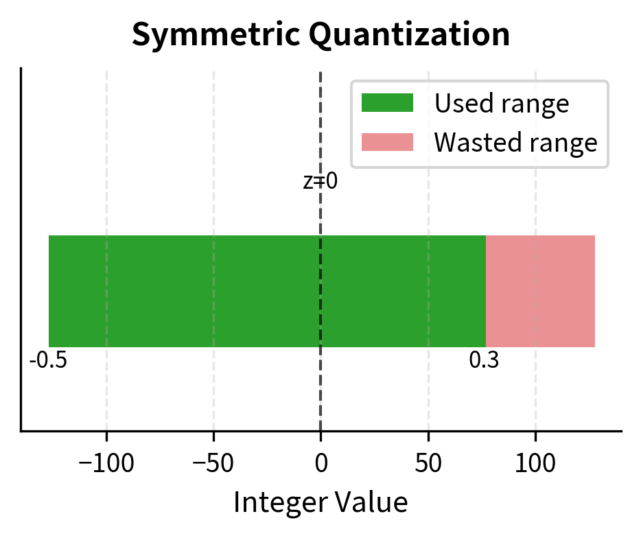
Symmetric quantization takes a simpler approach by forcing the zero-point to be zero (), which centers the quantized range around zero. This constraint means that real zero always maps to integer zero, creating a symmetric mapping where positive and negative values are treated identically. The scale is determined by the largest absolute value in the tensor:
where:
- : the scale factor
- : the maximum absolute value present in the tensor
- : the maximum positive integer in the target range
This formula ensures that the largest magnitude value, whether positive or negative, maps to the edge of the integer range. The symmetry comes from the fact that would map to , using the same scale factor.
For 8-bit signed integers with , a tensor with values in would use . This means:
- maps to
- maps to
- maps to
The main advantage of symmetric quantization is computational simplicity. With , the dequantization becomes a simple multiplication:
where:
- : the reconstructed real value
- : the scale factor
- : the quantized integer
This simplification significantly improves computational efficiency. Matrix multiplications can stay in integer arithmetic longer before converting back to floating point. When multiplying two symmetrically quantized matrices, we can perform the entire integer multiplication first, then apply the combined scale factor to the result. Many hardware accelerators, including tensor cores, are optimized for this pattern.
However, symmetric quantization wastes representable range when the tensor distribution is asymmetric. In our example, values only range up to 0.3, but we allocated integer range up to 76, leaving integers 77-127 unused. This effectively reduces the precision available for actual values. Those 51 unused integer levels represent wasted precision that could have been used to distinguish between values more finely.
Asymmetric Quantization
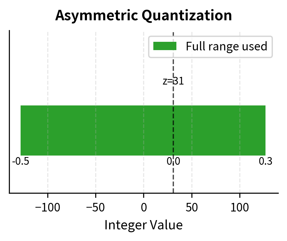
Asymmetric quantization removes the symmetry constraint, allowing a non-zero and thereby using the full integer range for the actual value distribution. This flexibility comes at the cost of additional complexity but provides better precision when the data distribution is skewed.
For our tensor with values in :
Now:
- maps to
- maps to
- maps to
The full integer range is utilized, providing finer resolution. The scale is 0.00314 instead of 0.00394, meaning each integer step represents a smaller real interval and quantization error is reduced. This improvement of approximately 20% in scale translates directly to a 20% reduction in maximum quantization error per value.
The tradeoff is computational complexity. The zero-point must be tracked and subtracted during dequantization or matrix operations. This adds overhead and can complicate hardware-optimized kernels. Additionally, the zero-point requires storage alongside the scale. For matrix multiplication between two asymmetrically quantized matrices, the computation involves cross-terms between values and zero-points that don't appear in the symmetric case.
Choosing Between Schemes
The choice depends on the tensor distribution and hardware constraints:
- Weights often follow approximately symmetric distributions centered near zero, making symmetric quantization effective with minimal range waste
- Activations frequently have asymmetric distributions, especially after ReLU (all positive) or after certain normalization layers. Asymmetric quantization better captures these distributions
- Hardware support varies. Some accelerators handle symmetric quantization much more efficiently, making it preferable even when asymmetric would be theoretically better
In practice, weight quantization commonly uses symmetric schemes while activation quantization uses asymmetric schemes, though this varies by implementation. The decision ultimately balances mathematical optimality against engineering constraints, and different deployment scenarios may favor different choices.
Per-Tensor vs Per-Channel Quantization
Beyond the symmetric/asymmetric choice, we must decide the granularity at which to compute quantization parameters. Should a single scale cover an entire weight matrix, or should different parts of the matrix have different scales? This decision profoundly affects both quantization accuracy and storage overhead.
Per-Tensor Quantization
The simplest approach computes one scale (and possibly one zero-point) for an entire tensor. All elements share the same quantization mapping, which means every value in the tensor is quantized using identical parameters.
This is memory-efficient: a weight matrix with millions of elements needs only 1-2 extra parameters for quantization. The overhead is essentially zero. However, if different regions of the tensor have very different value ranges, per-tensor quantization performs poorly. Outliers force a large scale, reducing precision for the majority of values.
Consider a weight matrix where most values fall in but a few outliers reach . Per-tensor symmetric 8-bit quantization uses . Values of 0.05 quantize to and dequantize to approximately 0.047. The relative error is 6%. Meanwhile, the outlier at 1.0 maps perfectly to 127. The common-case values suffer large relative errors to accommodate rare outliers.
This phenomenon illustrates a fundamental tradeoff in quantization: we must balance precision across the entire value distribution. When a single scale must serve all values, extreme values dictate the scale, and typical values pay the precision penalty.
Per-Channel Quantization
Per-channel quantization addresses this limitation by computing separate scales for each output channel of a weight tensor. For a linear layer with weight matrix (where is the output dimension and is the input dimension), we compute different scales, one per row.
This allows each output neuron's weights to use the full integer range based on that neuron's specific value distribution. If neuron 0 has weights in and neuron 1 has weights in , they get scales of approximately 0.00079 and 0.00787 respectively. Each achieves good precision for its own distribution, without being penalized by the other's characteristics.
The cost is storing scale values instead of 1. For typical transformer dimensions, this is negligible: a 4096-dimensional layer adds 4096 floats (16 KB) to store scales, while the weight matrix itself contains elements (8 MB at 4-bit). The overhead is well under 1%. This small cost buys significant accuracy improvements.
Per-Group Quantization
An intermediate approach divides each channel into groups of fixed size (commonly 32 or 128 elements) and computes scales per group. This handles within-channel variation while keeping overhead manageable. The group size represents a tunable parameter that balances precision against storage.
For a matrix with group size 128, we need scale values. At FP16, this adds 262 KB of overhead (roughly 3% of the 4-bit weight size). The finer granularity better handles outliers without significantly inflating storage.
Per-group quantization has become standard in aggressive 4-bit quantization schemes like GPTQ and AWQ, which we'll cover in upcoming chapters. The additional precision from per-group scales often makes the difference between acceptable and unacceptable accuracy loss. When pushing to very low bit widths, every bit of precision matters, and per-group quantization provides a reliable way to recover precision lost to value distribution variations.
Calibration
The process of determining optimal quantization parameters (scale, zero-point, or clipping thresholds) by analyzing the actual value distributions in a model, typically using representative input data.
We've assumed we know the minimum and maximum values of each tensor, but finding these optimally requires care. Simply taking the observed min/max may not be ideal, especially for activations that vary with input data. Calibration is the process of determining these parameters systematically, and the quality of calibration directly impacts quantized model accuracy.
Weight Calibration
Weights are fixed after training, so their distributions are known exactly. For per-tensor quantization, we can directly compute global min/max. For per-channel or per-group, we compute statistics for each partition. Since weights don't change during inference, calibration happens once and the parameters are stored with the model.
However, raw min/max may be skewed by rare extreme values. Some methods clip the range to exclude extreme outliers, accepting large errors on those values in exchange for better precision on typical values. The reasoning is that if only 0.1% of values are extreme, accepting large errors on those values while improving precision for the other 99.9% reduces overall error. Common approaches include:
- Percentile clipping: Use the 99.9th percentile instead of the true maximum, sacrificing outlier accuracy
- MSE minimization: Search for the clipping threshold that minimizes mean squared quantization error over the tensor
- Entropy-based: Choose thresholds that minimize KL divergence between original and quantized distributions
Activation Calibration
Activations present a harder problem because their distributions depend on inputs. A model might produce activations ranging from to on one input and to on another. We need to find quantization parameters that work well across the expected input distribution, not just for any single input.
The standard approach runs the model on a calibration dataset: a small representative sample of inputs. We collect activation statistics (min, max, percentiles, or full histograms) across this dataset, then compute quantization parameters from the aggregated statistics. The calibration dataset serves as a proxy for the true inference distribution.
Common aggregation strategies include:
- Running min/max: Track the most extreme values seen across all calibration samples
- Moving average: Smooth the statistics across samples to reduce sensitivity to outliers
- Histogram-based: Build full histograms and choose optimal thresholds by minimizing reconstruction error
The calibration dataset should resemble actual inference inputs. Using the wrong distribution during calibration can lead to clipping or range waste during deployment. A few hundred to a few thousand samples typically suffice for stable statistics, though the exact number depends on how variable the activations are.
Dynamic vs Static Quantization
Calibration determines whether quantization is static or dynamic:
-
Static quantization fixes all quantization parameters at calibration time. Inference uses predetermined scales and zero-points, with no runtime overhead for parameter computation. This is efficient but may lose accuracy if inference distributions differ from calibration.
-
Dynamic quantization computes activation quantization parameters on-the-fly for each input. This adapts to the actual values but adds overhead for computing statistics during inference. It's commonly used when activation distributions are highly variable.
Weight quantization is almost always static since weights don't change. Activation quantization may be either, depending on the accuracy-efficiency tradeoff desired.
Implementation
Let's implement the core quantization operations to solidify these concepts. We'll start with basic symmetric quantization, then extend to asymmetric and per-channel variants. Working through concrete code helps build intuition for how the mathematical formulas translate to practice.
The weights follow a roughly symmetric distribution centered near zero, typical of neural network parameters after initialization or training. This distribution is well-suited to symmetric quantization, which we will implement first.
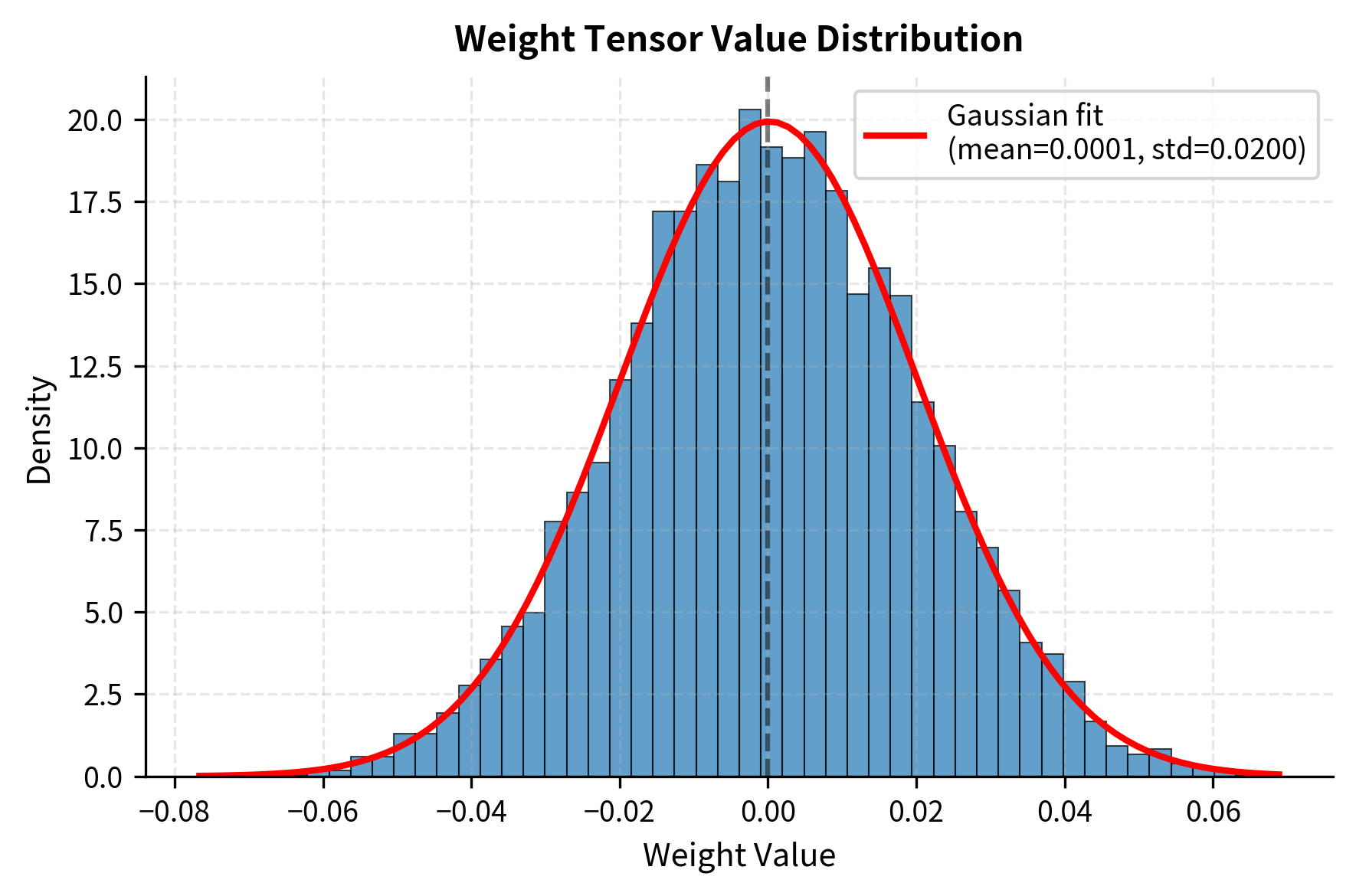
Symmetric Per-Tensor Quantization
The symmetric per-tensor implementation demonstrates the simplest form of quantization. We compute a single scale from the maximum absolute value, then apply the same quantization formula to every element in the tensor.
The mean absolute error is small compared to the weight standard deviation. 8-bit symmetric quantization preserves weights well when the distribution is roughly symmetric. The relative error of less than 1% indicates that the quantized weights closely approximate the originals, which bodes well for maintaining model accuracy.
Asymmetric Per-Tensor Quantization
The asymmetric implementation adds complexity by computing and tracking a zero-point. This extra parameter allows better use of the integer range when values are not centered at zero.
For this symmetric weight distribution, asymmetric quantization provides similar accuracy to symmetric. The zero-point is near 128, roughly the middle of the unsigned range, as expected for zero-centered data. When the data is already symmetric, asymmetric quantization offers little benefit but also causes no harm.
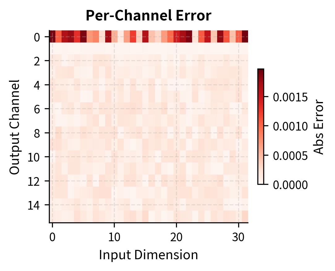
Per-Channel Quantization
Per-channel quantization computes separate scales for each row of the weight matrix, allowing each output channel to use its full precision budget independently.
To illustrate the benefits of per-channel quantization, we create a tensor where different channels have dramatically different value ranges. This simulates the real-world situation where some neurons develop larger weights than others during training.
Per-channel quantization dramatically reduces error for channel 1. With per-tensor quantization, the large channel forces a big scale, causing the small channel to quantize coarsely. Per-channel quantization gives each channel an appropriate scale. The error reduction for channel 1 can be several orders of magnitude, demonstrating why per-channel quantization is essential for high-accuracy quantization.
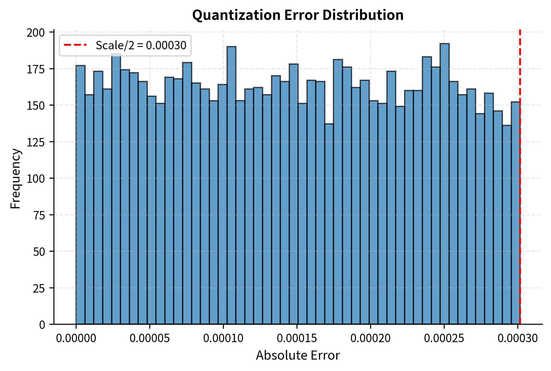
Visualizing Quantization Error
Visualization helps build intuition about how quantization errors distribute across values. The following plots show both the error distribution and the relationship between original and reconstructed values.
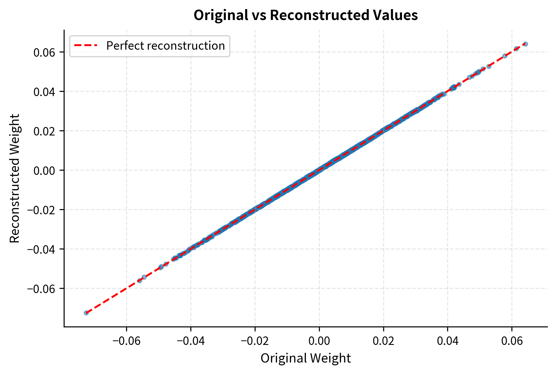
The error histogram shows that quantization errors are bounded and mostly small. The maximum possible error is half the scale (when a value falls exactly between two quantization levels). The scatter plot confirms tight correlation between original and reconstructed values, with points clustering closely around the diagonal line that represents perfect reconstruction.
Simulating Calibration
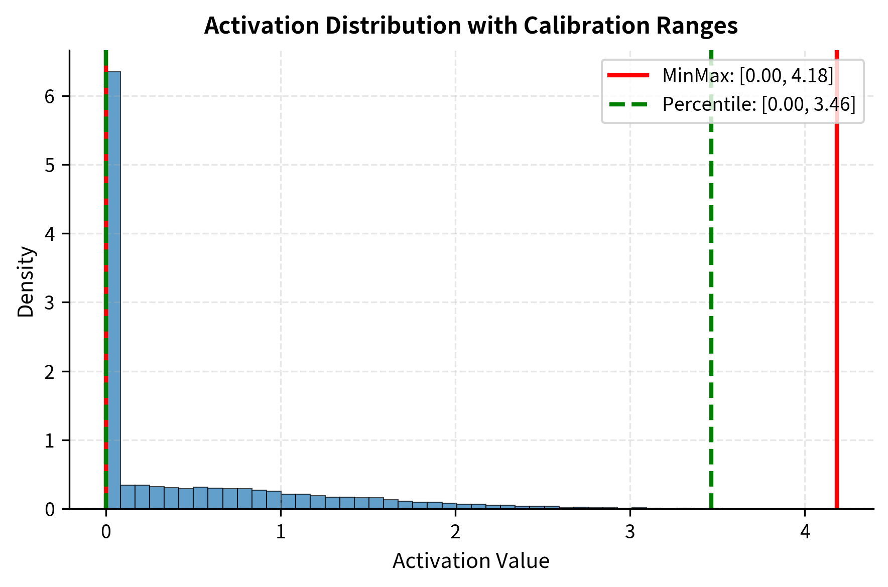
Calibration in practice involves running the model on representative data to collect statistics. The following code simulates this process for a simple model, demonstrating both minmax and percentile-based calibration approaches.
Percentile-based calibration produces a smaller scale, providing finer quantization resolution for the bulk of activations at the cost of clipping rare outliers. The scale reduction directly translates to smaller quantization errors for typical values, which usually improves overall model accuracy.
Comparing Bit Widths
The following experiment measures how quantization error changes with bit width, demonstrating the exponential relationship between precision and error.
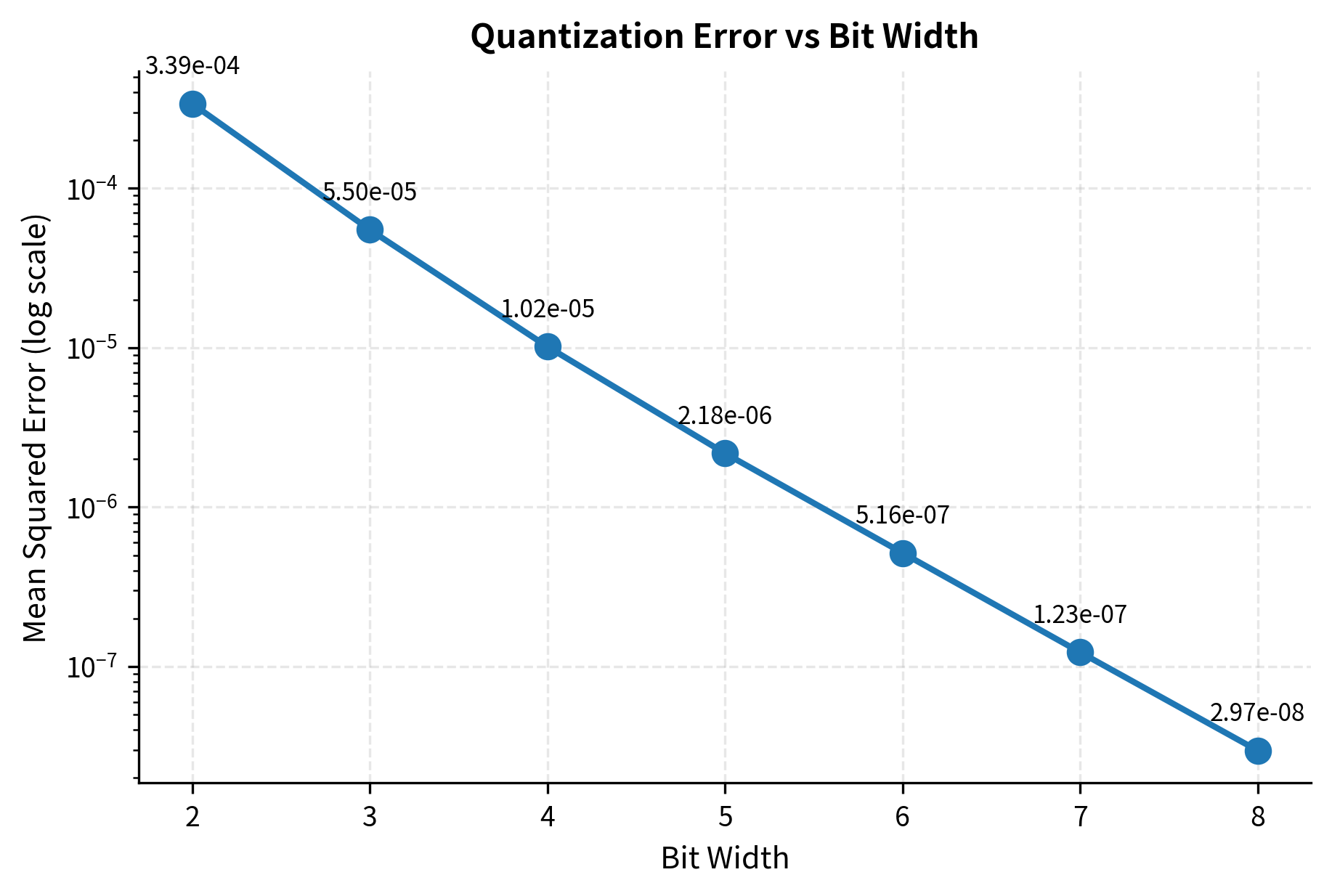
Error drops roughly by a factor of 4 for each additional bit. This follows from quantization theory: each extra bit doubles the number of representable levels, halving the quantization step size, which reduces mean squared error by a factor of 4. This relationship helps you make informed decisions about the precision-accuracy tradeoff for your specific applications.
Key Parameters
The key parameters for the quantization functions are:
- num_bits: The bit width for the target integer representation (e.g., 8 for INT8, 4 for INT4). Lower bits increase compression but reduce precision.
- axis: The dimension along which quantization parameters (scale, zero-point) are computed. For per-channel quantization of Linear layers, this is typically the output dimension (axis 0).
- method: The strategy for determining quantization ranges during calibration (e.g., 'minmax' or 'percentile').
Limitations and Practical Considerations
Quantization's appeal lies in its simplicity, but several challenges arise in practice.
Outlier sensitivity remains the primary obstacle to aggressive quantization. Transformer models frequently develop weight and activation outliers during training. A single extreme value in a tensor can force a large scale, wasting precision for all other values. Per-channel and per-group quantization mitigate this for weights, but handling activation outliers often requires more sophisticated techniques. Methods like LLM.int8() detect outliers at runtime and process them in higher precision, while AWQ and GPTQ (covered in upcoming chapters) use careful calibration to minimize outlier impact.
Accuracy degradation varies dramatically across models and tasks. Simple tasks like classification often tolerate aggressive quantization with minimal accuracy loss. Generation tasks, especially those requiring precise reasoning or factual recall, prove more sensitive. A model that performs well on perplexity benchmarks after 4-bit quantization may show subtle degradation in reasoning quality or factual consistency. Always evaluate on task-specific metrics, not just generic benchmarks.
Calibration dataset selection significantly impacts results. Using the wrong distribution during calibration can cause systematic clipping or range waste during deployment. For general-purpose models, calibration data should span the expected input distribution. For specialized applications, calibration on domain-specific data often yields better results than generic calibration.
Hardware support determines practical speedup. Integer operations are only faster if the hardware has efficient integer compute units. Modern GPUs offer accelerated INT8 and sometimes INT4 operations through tensor cores, but not all hardware supports all quantization formats. Some quantization schemes that theoretically reduce compute find no actual speedup due to missing hardware support or kernel availability.
Despite these challenges, quantization has enabled an explosion in LLM accessibility. Models that required enterprise-grade hardware now run on laptops and smartphones. The memory savings cascade into reduced serving costs, making AI applications economically viable at scales previously impossible. The next chapters will explore specific quantization methods, INT8 and INT4 techniques, and formats like GPTQ and AWQ that push compression further while maintaining accuracy.
Summary
Quantization maps high-precision floating-point values to lower-precision integers, reducing memory footprint and often enabling faster computation. The core operation involves a scale (determining step size) and optionally a zero-point (shifting the mapping), with the choice between symmetric and asymmetric schemes trading simplicity against representation efficiency.
Quantization granularity ranges from per-tensor (one scale for all values) through per-channel (one scale per output dimension) to per-group (multiple scales within each channel). Finer granularity better handles value distribution variations at the cost of additional scale storage.
Calibration determines optimal quantization parameters by analyzing actual tensor values. For weights, this is straightforward since values are fixed. For activations, running the model on representative calibration data provides necessary statistics. Methods like percentile clipping can improve results by trading accuracy on rare outliers for better precision on common values.
The fundamental tradeoff in quantization is information loss versus compression. Fewer bits mean smaller models and faster inference but increased quantization error. Understanding this tradeoff, and the tools for managing it, prepares you for the specific quantization techniques in the following chapters.
Quiz
Ready to test your understanding? Take this quick quiz to reinforce what you've learned about weight quantization fundamentals.

Comments