

A comprehensive guide covering LightGBM gradient boosting framework, including leaf-wise tree growth, histogram-based binning, GOSS sampling, exclusive feature bundling, mathematical foundations, and Python implementation. Learn how to use LightGBM for large-scale machine learning with speed and memory efficiency.

This article is part of the free-to-read Machine Learning from Scratch
Choose your expertise level to adjust how many terms are explained. Beginners see more tooltips, experts see fewer to maintain reading flow. Hover over underlined terms for instant definitions.
LightGBM
LightGBM (Light Gradient Boosting Machine) is a highly efficient gradient boosting framework that builds upon the foundation of boosted trees while introducing several key innovations that make it particularly well-suited for large-scale machine learning tasks. As we've already explored boosted trees, we understand that gradient boosting combines multiple weak learners (typically decision trees) in a sequential manner, where each new tree corrects the errors of the previous ensemble. LightGBM takes this concept and optimizes it for both speed and memory efficiency through novel tree construction algorithms and data handling techniques.
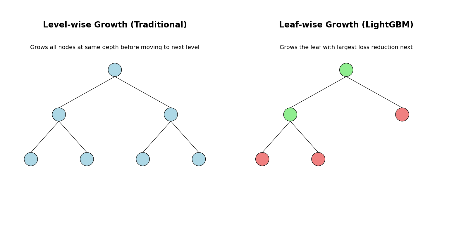
The primary innovation that sets LightGBM apart is its use of leaf-wise tree growth instead of the traditional level-wise approach. While conventional gradient boosting methods like XGBoost grow trees level by level (expanding all nodes at the same depth before moving to the next level), LightGBM grows trees by selecting the leaf with the largest loss reduction to split next. This approach can lead to more complex trees that achieve the same accuracy with fewer total nodes, resulting in faster training and prediction times.
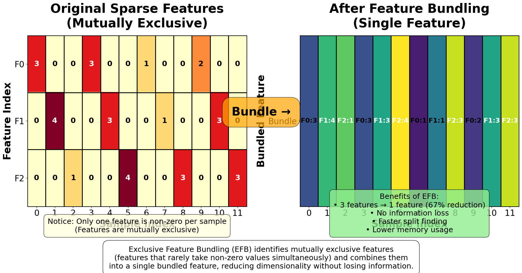
Another key differentiator is LightGBM's Gradient-based One-Side Sampling (GOSS) and Exclusive Feature Bundling (EFB) techniques. GOSS focuses training on instances with larger gradients (harder-to-predict samples) while randomly sampling instances with smaller gradients, effectively reducing the computational cost without significantly impacting model quality. EFB reduces the number of features by bundling mutually exclusive features together, which is particularly beneficial for high-dimensional sparse datasets commonly found in real-world applications.
We will not cover learning to rank in this course. However, it is important to note that LightGBM is widely used for learning to rank tasks, such as information retrieval and recommendation systems. LightGBM's ranking implementation is similar in principle to XGBoost's, but it includes its own optimizations and ranking objectives (such as lambdarank and rank_xendcg) that are specifically tailored for efficient and scalable ranking model training.
Advantages
LightGBM offers several compelling advantages that make it an excellent choice for many machine learning scenarios. The most significant benefit is its exceptional computational efficiency - LightGBM can be significantly faster than traditional gradient boosting methods while using less memory, with speed improvements of 2-10x depending on the dataset characteristics.
Note: Performance improvements vary significantly based on dataset size, dimensionality, and hardware. LightGBM's advantages are most pronounced with large datasets (millions of samples) and high-dimensional sparse data.
This speed advantage comes from multiple sources: the leaf-wise tree growth strategy, optimized histogram-based algorithms for finding the best splits, and efficient parallel computing implementations that can utilize multiple CPU cores effectively.
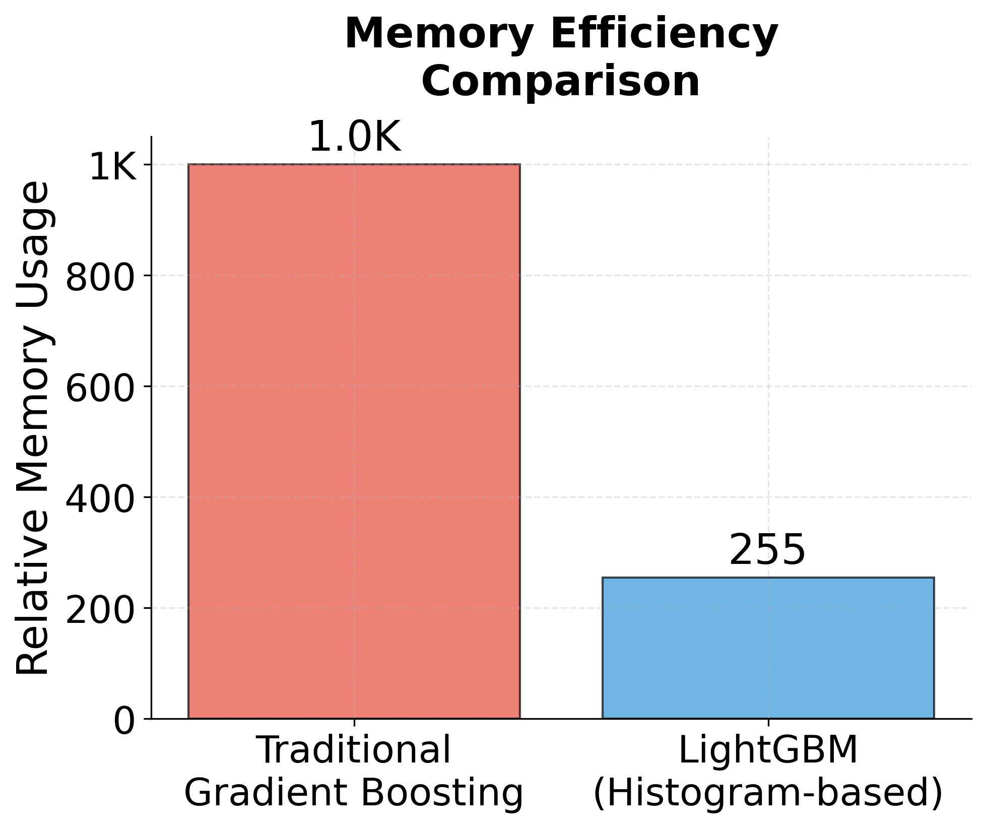
The framework's memory efficiency is particularly noteworthy for large-scale applications. LightGBM uses a novel histogram-based approach for split finding that requires much less memory than traditional methods. Instead of storing all possible split points, it discretizes continuous features into bins and works with these histograms, dramatically reducing memory requirements. This makes LightGBM practical for datasets that would be too large to fit in memory using other gradient boosting implementations.
LightGBM also provides excellent out-of-the-box performance with minimal hyperparameter tuning. The default parameters are well-optimized for most use cases, and the framework includes built-in support for categorical features without requiring one-hot encoding, which can significantly reduce preprocessing time and memory usage. Additionally, LightGBM offers robust handling of missing values and can automatically learn optimal strategies for dealing with them during training.
Disadvantages
Despite its many advantages, LightGBM does have some limitations that practitioners should be aware of. The leaf-wise tree growth strategy, while efficient, can lead to overfitting more easily than level-wise growth, especially on smaller datasets. This means that LightGBM may require more careful regularization and early stopping compared to other gradient boosting methods, and it might not be the best choice for very small datasets where the risk of overfitting is high.
Another potential drawback is that LightGBM's optimizations, while excellent for speed and memory efficiency, can sometimes make the model less interpretable than simpler alternatives. The leaf-wise growth and feature bundling techniques can create more complex tree structures that are harder to visualize and understand. For applications where model interpretability is crucial, simpler methods like traditional decision trees or even XGBoost with level-wise growth might be more appropriate.
LightGBM also has some limitations in terms of algorithm diversity compared to other frameworks. While it excels at gradient boosting, it doesn't offer the same variety of base learners or boosting algorithms that some other frameworks provide. Additionally, the framework's focus on efficiency sometimes comes at the cost of flexibility - certain advanced features or custom loss functions that might be available in other frameworks may not be as easily implemented in LightGBM.
Understanding Bins
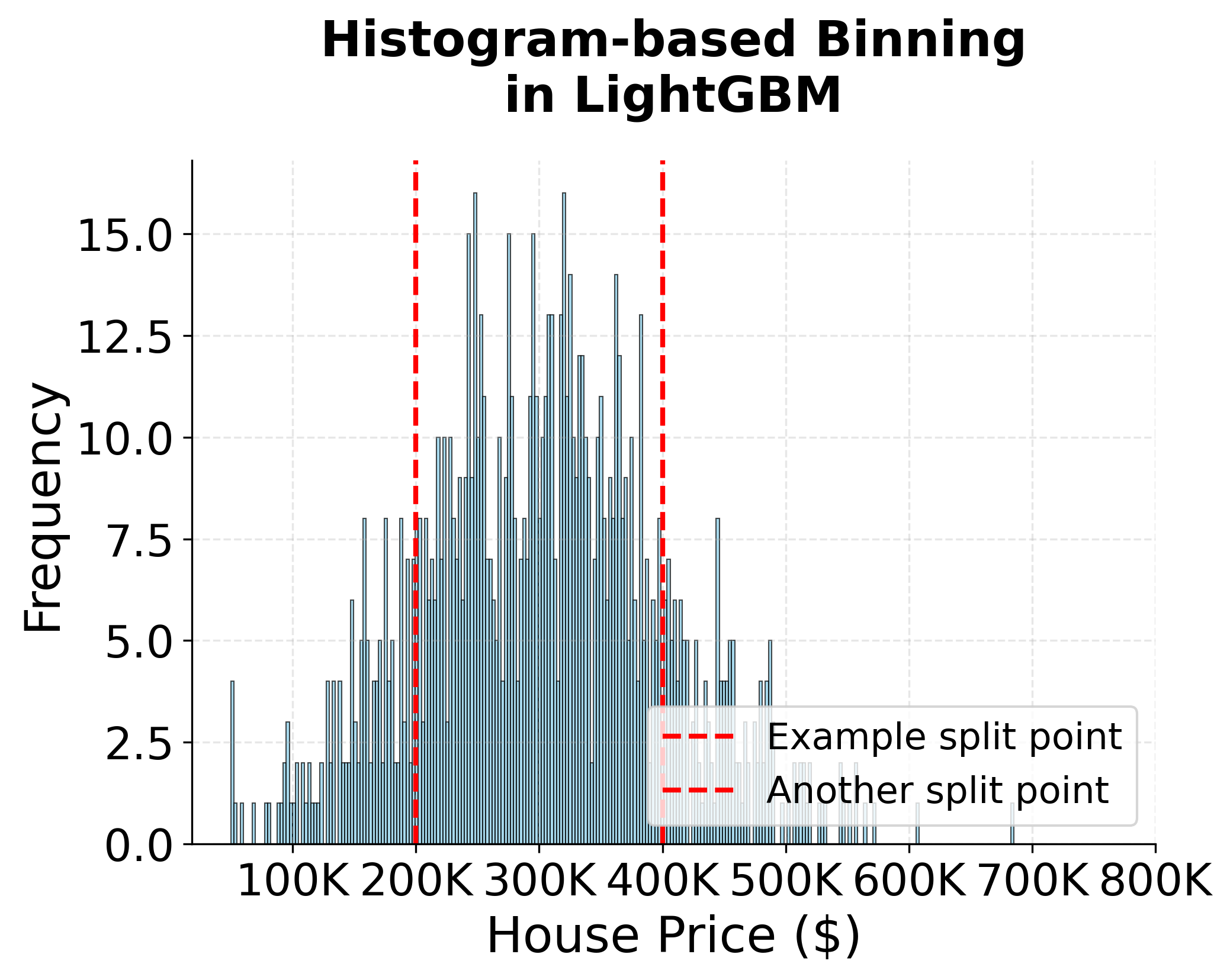
The concept of bins is fundamental to understanding how LightGBM achieves its remarkable efficiency. In traditional gradient boosting methods like XGBoost, the algorithm must evaluate every possible split point for continuous features, which can be computationally expensive for large datasets. LightGBM revolutionizes this process through histogram-based binning.
Bins are essentially discrete intervals that divide the range of continuous feature values into a fixed number of buckets. For example, if we have a feature representing house prices ranging from 500,000, we might create 255 bins (the default in LightGBM), where each bin represents a price range of approximately 50,000 and 51,765 and $53,530 into the second bin, and so on.
How binning works in practice:
- Feature Discretization: For each continuous feature, LightGBM automatically determines the optimal number of bins (default is 255) and creates histogram buckets that cover the entire range of feature values.
- Gradient Accumulation: Instead of tracking gradients for individual data points, LightGBM accumulates gradients and Hessians within each bin. This means that all data points falling into the same bin are treated as having the same feature value for split evaluation purposes.
- Split Evaluation: When finding the best split, LightGBM only needs to evaluate splits at bin boundaries rather than at every possible data point. This dramatically reduces the number of split candidates from potentially thousands to just 255 (or whatever the bin count is).
Memory and computational benefits:
- Memory efficiency: Instead of storing gradients for every data point, LightGBM only needs to store gradient sums for each bin, reducing memory usage from to where is the number of samples and is the number of features.
- Computational speed: Evaluating splits at bin boundaries is much faster than evaluating every possible split point, especially for large datasets.
- Approximation quality: While binning introduces some approximation error, the default of 255 bins provides excellent accuracy while maintaining significant efficiency gains.
Adaptive binning: LightGBM uses sophisticated algorithms to determine optimal bin boundaries. It can handle different distributions of feature values and automatically adjusts bin sizes to ensure that each bin contains a reasonable number of data points. This adaptive approach helps maintain model accuracy even with the discretization process.
The binning strategy is particularly effective for high-cardinality categorical features as well. Instead of creating one-hot encoded features (which would be memory-intensive), LightGBM can directly work with categorical values by treating them as discrete bins, further enhancing efficiency.
Formula
The mathematical foundation of LightGBM builds upon the standard gradient boosting framework, but with key modifications to the tree construction process. Let's start with the fundamental gradient boosting objective function and then see how LightGBM optimizes it.
Note: The Loss function should look very similar to the one in XGBoost, hence we will not repeat the details here. Please refer to the XGBoost section for more detail.
The standard gradient boosting objective function combines a loss function with regularization terms:
where is the loss function, is the -th tree we're adding, and is the regularization term for the tree.
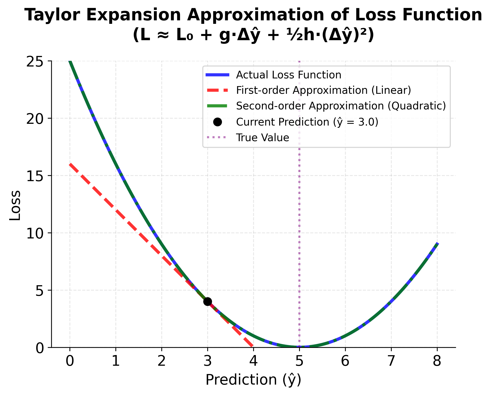
In LightGBM, we use a second-order Taylor expansion to approximate this objective:
where:
- : first-order gradient (the slope of the loss function with respect to the prediction for instance )
- : second-order gradient or Hessian (the curvature of the loss function with respect to the prediction for instance )
This second-order approximation provides a more accurate representation of the loss function around the current prediction.
The key innovation in LightGBM lies in its unique approach to constructing decision trees, which is fundamentally different from the traditional level-wise method used in most gradient boosting frameworks.
Let's break down the LightGBM tree construction process step by step:
-
Leaf-wise Growth Strategy:
- In traditional level-wise tree growth (as in XGBoost by default), all leaves at the current depth are split simultaneously, resulting in a balanced tree.
- LightGBM, however, adopts a leaf-wise (best-first) growth strategy. At each step, it searches among all current leaves and selects the one whose split would result in the largest reduction in the loss function (i.e., the greatest "gain").
- This means that LightGBM can grow deeper, more complex branches where the model can most effectively reduce error, potentially leading to higher accuracy with fewer trees.
-
Calculating the Split Gain:
- When considering splitting a particular leaf , LightGBM evaluates all possible splits and calculates the "gain" for each.
- The gain measures how much the split would reduce the overall loss function. The formula for the gain when splitting a leaf into left () and right () children is:
where:
- : first-order gradient (the derivative of the loss with respect to the prediction for instance )
- : second-order gradient (the second derivative, or curvature, of the loss for instance )
- : set of all instances in the current leaf before the split
- : set of instances that would go to the left child leaf after the split
- : set of instances that would go to the right child leaf after the split
- : L2 regularization parameter (helps prevent overfitting by penalizing large leaf weights)
- : minimum gain threshold required to make a split (splits with gain less than are not performed)
Observe that in the gain formula, each term of the form represents a fraction: the numerator is the square of the sum of gradients for a group of instances (such as all instances in the left child), and the denominator is the sum of the Hessians (second-order gradients) for those instances plus the regularization parameter .
This fraction reflects the confidence in the leaf's prediction—a larger sum of gradients (numerator) indicates a greater potential adjustment, while a larger sum of Hessians (denominator) or stronger regularization reduces the magnitude of that adjustment. The difference between the fractions for the left and right children and the original leaf quantifies the net reduction in loss achieved by making the split.
- Step-by-step Gain Calculation:
- a. For each possible split, sum the gradients () and Hessians () for the left and right child nodes.
- b. Compute the gain for the split using the formula above.
- c. Compare the gain to the threshold . If the gain is greater than , the split is considered valid.
- d. Among all possible splits across all leaves, select the split with the highest gain and perform it.
- e. Repeat this process, always splitting the leaf with the largest potential gain, until a stopping criterion is met (such as maximum tree depth, minimum number of samples in a leaf, or minimum gain).
This leaf-wise, best-first approach allows LightGBM to focus its modeling capacity where it is most needed, often resulting in faster convergence and higher accuracy compared to level-wise methods. However, because it can create deeper, more complex trees, it may also be more prone to overfitting, especially on small datasets—so regularization and early stopping are important.
In summary, LightGBM's step-by-step tree construction process is:
- At each iteration, evaluate all possible splits for all current leaves.
- Calculate the gain for each split using the gradients and Hessians.
- Select and perform the split with the highest gain (if it exceeds ).
- Repeat until stopping criteria are met.
This process is at the heart of LightGBM's efficiency and predictive power.
The Gradient-based One-Side Sampling (GOSS) technique is a core innovation in LightGBM that significantly accelerates training without sacrificing accuracy, especially on large datasets. GOSS is based on the observation that data instances with larger gradients (i.e., those that are currently poorly predicted by the model) contribute more to the information gain when building trees. Therefore, GOSS prioritizes these "hard" instances during the split-finding process.
Here's how GOSS works in detail:
-
Gradient Calculation:
- For each data instance, compute the gradient of the loss function with respect to the current prediction. The magnitude of the gradient reflects how much the model's prediction for that instance needs to be updated.
-
Instance Selection:
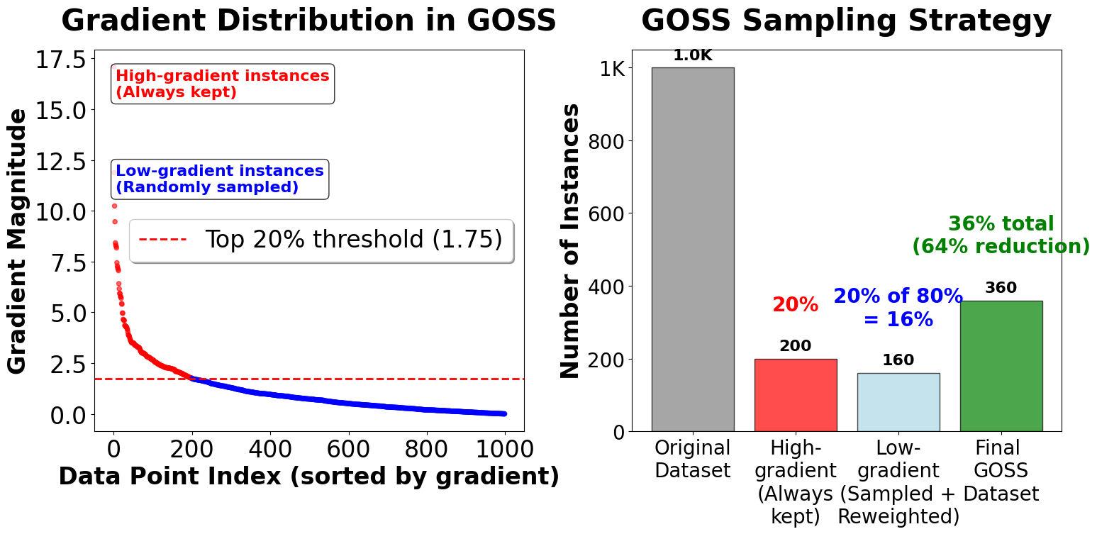
- Large-gradient instances: Select and retain all instances whose gradients are among the top fraction (e.g., the top 20%) of all gradients. These are the most "informative" samples for the current boosting iteration.
- Small-gradient instances: From the remaining instances (those with smaller gradients), randomly sample a subset, typically a fraction (e.g., 20%) of the total data. This ensures that the model still sees a representative sample of "easy" instances, but at a much lower computational cost.
-
Reweighting for Unbiased Estimation:
- Because the small-gradient instances are under-sampled, GOSS compensates by up-weighting their gradients and Hessians during the split gain calculation. Specifically, the gradients and Hessians of the randomly sampled small-gradient instances are multiplied by a factor of to ensure that the overall distribution of gradients remains unbiased.
Note: The reweighting factor ensures that the expected contribution of small-gradient instances matches what would be obtained from the full dataset, maintaining the statistical properties of the gradient boosting algorithm.
- Split Finding:
- The split-finding process (i.e., evaluating possible feature splits and calculating the gain for each) is then performed using the union of all large-gradient instances and the sampled, reweighted small-gradient instances. This dramatically reduces the number of data points considered at each split, leading to much faster training.
The sampling ratio for small-gradient instances is typically set to , where is the sampling ratio for large-gradient instances and is the sampling ratio for small-gradient instances. For example, if and , then 20% of the data with the largest gradients are retained, and 20% of the remaining data with small gradients are randomly sampled and up-weighted.
The Gradient-based One-Side Sampling (GOSS) technique offers several important advantages. First, it greatly improves efficiency by concentrating computational effort on the most informative samples—those with the largest gradients—thereby reducing the amount of data that needs to be processed at each iteration and resulting in faster training times. Second, GOSS maintains high accuracy because it includes all large-gradient instances, ensuring that the model continues to learn from the most challenging and informative cases without losing critical information. Finally, the reweighting of the randomly sampled small-gradient instances guarantees that the calculation of split gain remains an unbiased estimate of what would be obtained if the full dataset were used, preserving the integrity of the learning process.
In summary, GOSS enables LightGBM to scale to very large datasets by reducing the computational burden of split finding, while still preserving the accuracy and robustness of the model.
Mathematical properties
LightGBM maintains the convergence guarantees of gradient boosting, while introducing several efficiency improvements. Its leaf-wise tree growth strategy often results in faster convergence (fewer trees required for a given level of accuracy), though it necessitates careful regularization to avoid overfitting. The histogram-based split finding algorithm in LightGBM has a time complexity of , which is generally more efficient than the complexity of traditional pre-sorted algorithms, especially when the number of bins is much smaller than the number of data points.
In terms of memory usage, LightGBM scales as , rather than , making it well-suited for high-dimensional data. Additionally, the Exclusive Feature Bundling (EFB) technique can reduce the effective number of features by combining mutually exclusive (non-overlapping) features, sometimes halving the number of features in sparse datasets and further improving memory and computational efficiency.
Visualizing LightGBM
Let's create visualizations that demonstrate LightGBM's key characteristics and performance advantages.
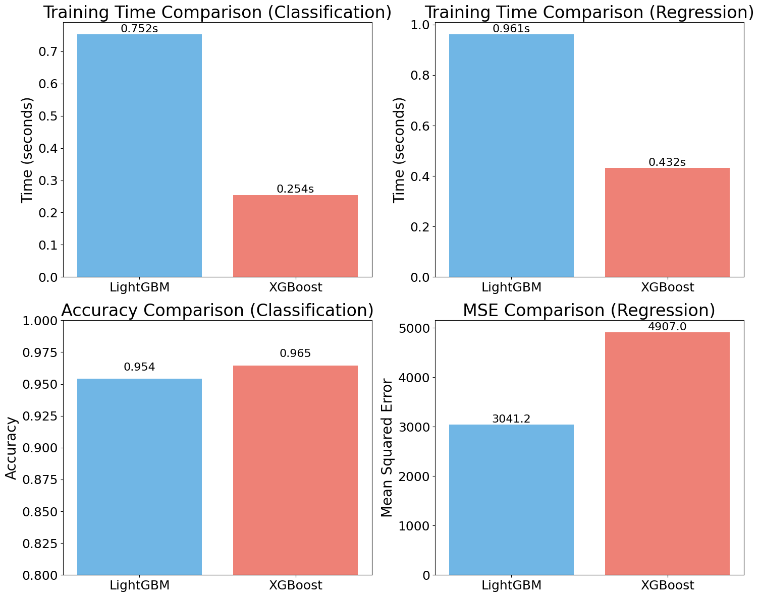
Note: The performance comparison below uses relatively small synthetic datasets (10,000 samples, 20 features) for demonstration purposes. LightGBM's true advantages become more apparent with larger, real-world datasets containing millions of samples and hundreds or thousands of features.
Note: The results presented above may seem unexpected, especially considering LightGBM's strong reputation for speed and efficiency. However, several key factors help explain why XGBoost outperformed LightGBM in three out of four metrics in this particular comparison.
The results presented above may seem unexpected, especially considering LightGBM's strong reputation for speed and efficiency. However, several key factors help explain why XGBoost outperformed LightGBM in three out of four metrics in this particular comparison.
First, the characteristics of the datasets play a significant role. In this case, the synthetic datasets generated with make_classification and make_regression are relatively small, each containing 10,000 samples and 20 features. LightGBM's strengths are most pronounced with much larger datasets—those with millions of samples—and with higher-dimensional data. On smaller datasets, the overhead introduced by LightGBM's histogram-based binning and its leaf-wise tree growth strategy can sometimes outweigh the performance benefits these features provide.
Second, differences in default parameters between the two models can influence results. Both LightGBM and XGBoost were used with their default settings, but these defaults are optimized for different scenarios. XGBoost's default parameters may be better suited to the size and complexity of the datasets used here, while LightGBM's defaults—such as num_leaves=31—are designed for larger datasets where its efficiency advantages are more likely to be realized.
In summary, LightGBM's true advantages become most apparent in situations involving large datasets (over 100,000 samples), high-dimensional data (over 1,000 features), or sparse datasets, where its histogram-based approach and Exclusive Feature Bundling (EFB) offer significant benefits. Additionally, LightGBM excels with categorical features due to its built-in handling (eliminating the need for one-hot encoding) and is particularly well-suited for memory-constrained environments thanks to its lower memory footprint.
Example
Let's work through a concrete mathematical example to demonstrate how LightGBM builds trees and makes predictions. We'll use a simple regression problem with a small dataset to make the calculations transparent.
Note: This is a simplified pedagogical example designed to illustrate the core concepts. Real-world applications typically involve much larger datasets and more complex feature interactions.
Dataset
Suppose we have the following training data for predicting house prices based on size and age:
| House | Size (sq ft) | Age (years) | Price ($) |
|---|---|---|---|
| 1 | 100 | 5 | 200 |
| 2 | 150 | 10 | 280 |
| 3 | 200 | 2 | 350 |
| 4 | 120 | 8 | 220 |
| 5 | 180 | 15 | 300 |
| 6 | 250 | 1 | 450 |
| 7 | 140 | 12 | 260 |
| 8 | 160 | 6 | 290 |
Step 1: Initial Prediction and Gradient Calculation
The initial prediction for all samples is the mean of the target variable:
For regression with squared error loss, the gradient is the negative residual:
Example calculation for House 1:
- (actual price)
- (initial prediction)
Calculating gradients for each sample:
| House | |||
|---|---|---|---|
| 1 | 200 | 280 | 80 |
| 2 | 280 | 280 | 0 |
| 3 | 350 | 280 | -70 |
| 4 | 220 | 280 | 60 |
| 5 | 300 | 280 | -20 |
| 6 | 450 | 280 | -170 |
| 7 | 260 | 280 | 20 |
| 8 | 290 | 280 | -10 |
Step 2: Finding the Best Split
LightGBM evaluates potential splits and calculates the gain for each. Let's consider splitting on the 'size' feature. We sort the data by size and consider splits at midpoints between consecutive values:
| House | Size | Gradient |
|---|---|---|
| 1 | 100 | 80 |
| 4 | 120 | 60 |
| 7 | 140 | 20 |
| 2 | 150 | 0 |
| 8 | 160 | -10 |
| 5 | 180 | -20 |
| 3 | 200 | -70 |
| 6 | 250 | -170 |
Potential split points: 110, 130, 145, 155, 170, 190, 225
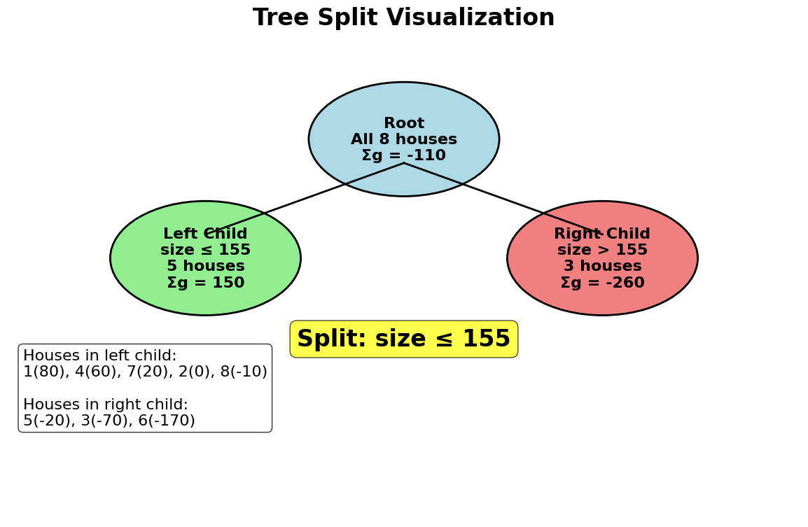
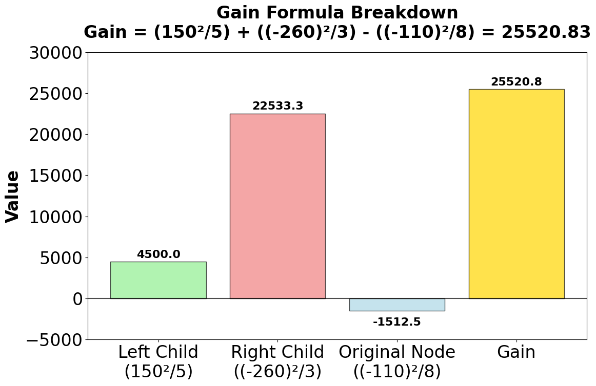
Let's calculate the gain for splitting at size ≤ 155:
Left child (size ≤ 155): Houses 1, 4, 7, 2, 8
Right child (size > 155): Houses 5, 3, 6
Original node:
Let's do the calculations step by step:
- Left child gradient sum:
- Right child gradient sum:
- Original node gradient sum:
Note: For this simplified example, we assume the Hessian (second-order gradient) equals 1 for all samples, which reduces the gain formula to a simpler form. In practice, LightGBM uses the full second-order approximation.
Using the simplified gain formula (assuming hessian = 1 for all samples):
The gain here quantifies how much the split at size ≤ 155 improves the model's objective function (i.e., reduces the loss) compared to not splitting. In gradient boosting, each split is chosen to maximize this gain, which represents the improvement in the model's fit to the data.
- A higher gain means the split creates child nodes that are more "pure" (i.e., the gradients within each child are more similar), leading to better predictions.
- The gain calculation uses the sum of gradients in each child and the parent, reflecting how well the split separates the data according to the current model's errors.
- In this example, a gain of 25,520.83 indicates a substantial reduction in the loss function, making this split highly desirable.
In summary, the gain measures the effectiveness of a split: the larger the gain, the more the split helps the model learn from the data.
Step 3: Leaf-wise Growth Decision
LightGBM would evaluate all possible splits and select the one with the highest gain. In this example, the split at size ≤ 155 shows a substantial gain of 25,520.83, indicating that this split significantly reduces the loss function.
The algorithm would then:
- Perform this split, creating two child nodes
- Continue the process by finding the next best split among all current leaves
- Focus on the leaf that would provide the largest gain reduction
This demonstrates how LightGBM's leaf-wise growth strategy prioritizes the most informative splits, building trees that focus computational effort where it can achieve the greatest loss reduction.
Implementation in LightGBM
LightGBM provides both a scikit-learn compatible interface and its native API. Let's demonstrate both approaches:
Scikit-learn Interface
The scikit-learn interface provides a familiar API for users already comfortable with scikit-learn. The accuracy score indicates strong predictive performance on this classification task. The classification report shows precision, recall, and F1-scores for each class, providing a comprehensive view of model performance across different metrics. High precision indicates that when the model predicts a class, it's usually correct, while high recall means the model successfully identifies most instances of each class.
Native LightGBM API
The native API offers more fine-grained control over the training process and is particularly useful for advanced users who need to customize training behavior. The model achieved comparable accuracy to the scikit-learn interface, demonstrating consistency across both APIs. The best iteration value shows where early stopping determined the optimal number of boosting rounds, helping prevent overfitting by stopping training when validation performance plateaus.
Feature Importance
Feature importance scores help identify which features contribute most to the model's predictions. Features with higher importance values have a stronger influence on the model's decision-making process. This information is valuable for feature selection, model interpretation, and understanding which aspects of your data drive predictions. In practice, you might consider removing features with very low importance to simplify the model without sacrificing performance.
Cross-Validation
Cross-validation provides a more robust estimate of model performance by evaluating the model on multiple train-test splits. The mean CV accuracy represents the average performance across all folds, while the standard deviation (shown as +/-) indicates the variability in performance. Low variability suggests the model performs consistently across different data subsets, which is a good indicator of generalization capability. If the CV scores vary significantly, it might indicate that the model is sensitive to the specific training data or that hyperparameter tuning is needed.
Key Parameters
Below are the main parameters that affect how LightGBM works and performs.
n_estimators: Number of boosting rounds or trees to build (default: 100). More trees generally improve performance but increase training time and memory usage. Start with 100 and increase if validation performance continues to improve.learning_rate: Step size shrinkage used to prevent overfitting (default: 0.1). Smaller values require more trees but often lead to better performance. Typical values range from 0.01 to 0.3.max_depth: Maximum depth of each tree (default: -1, meaning no limit). Limiting depth helps prevent overfitting. Values between 3 and 10 work well for most datasets.num_leaves: Maximum number of leaves in each tree (default: 31). This is the main parameter controlling tree complexity in LightGBM's leaf-wise growth. Should be less than to prevent overfitting.min_child_samples: Minimum number of samples required in a leaf node (default: 20). Higher values prevent overfitting by requiring more data support for splits. Increase for noisy data or small datasets.subsample(orbagging_fraction): Fraction of data to use for each tree (default: 1.0). Values less than 1.0 enable bagging, which can improve generalization. Typical values are 0.7 to 0.9.colsample_bytree(orfeature_fraction): Fraction of features to use for each tree (default: 1.0). Reduces correlation between trees and speeds up training. Values between 0.6 and 1.0 are common.reg_alpha: L1 regularization term (default: 0.0). Encourages sparsity in leaf weights. Useful for feature selection and preventing overfitting.reg_lambda: L2 regularization term (default: 0.0). Smooths leaf weights to prevent overfitting. More commonly used than L1 regularization.random_state: Seed for reproducibility (default: None). Set to an integer to ensure consistent results across runs.verbose: Controls the verbosity of training output (default: 1). Set to -1 to suppress all output, or higher values for more detailed logging.
Key Methods
The following are the most commonly used methods for interacting with LightGBM models.
fit(X, y): Trains the LightGBM model on training data X and target values y. Supports optional parameters likeeval_setfor validation data andcallbacksfor early stopping.predict(X): Returns predicted class labels (classification) or values (regression) for input data X. For classification, returns the class with the highest probability.predict_proba(X): Returns probability estimates for each class (classification only). Useful for setting custom decision thresholds or understanding prediction confidence.score(X, y): Returns the mean accuracy (classification) or R² score (regression) on the given test data. Convenient for quick model evaluation.feature_importances_: Property that returns the importance of each feature based on how often they are used for splitting. Higher values indicate more important features.
Practical Applications
Practical Implications
LightGBM excels in several specific scenarios where computational efficiency and scalability are paramount. Large-scale datasets with millions of samples and thousands of features represent a particularly well-suited use case for LightGBM, as its memory efficiency and speed advantages become most pronounced at this scale. The histogram-based approach and leaf-wise tree growth enable faster training compared to traditional gradient boosting methods, making it particularly valuable for companies processing big data in real-time or near real-time scenarios.
High-dimensional sparse data is another area where LightGBM demonstrates significant advantages. The Exclusive Feature Bundling (EFB) technique effectively handles datasets with many categorical variables or sparse features, such as those commonly found in recommendation systems, click-through rate prediction, and natural language processing applications. The framework's built-in categorical feature handling eliminates the need for one-hot encoding, reducing both memory usage and preprocessing time substantially.
Production environments with strict latency requirements benefit from LightGBM's fast prediction times. The leaf-wise tree growth strategy typically produces more compact trees with fewer total nodes, leading to faster inference compared to level-wise approaches. This makes LightGBM well-suited for applications like real-time fraud detection, dynamic pricing systems, and online advertising, where model predictions must be generated within milliseconds. However, practitioners should exercise caution when applying LightGBM to small datasets (typically less than 10,000 samples), as the leaf-wise growth strategy can lead to overfitting more easily than level-wise methods. For smaller datasets, simpler methods like logistic regression, random forests, or XGBoost with level-wise growth may be more appropriate.
Best Practices
To achieve optimal results with LightGBM, start by properly configuring the key hyperparameters. Begin with num_leaves=31 and max_depth=-1 (unlimited), but monitor for overfitting on smaller datasets by reducing num_leaves or setting a specific max_depth between 5 and 10. The learning rate should typically be set between 0.01 and 0.1, with lower values requiring more boosting rounds but often producing better generalization. Use early stopping with a validation set to automatically determine the optimal number of trees, setting callbacks=[lgb.early_stopping(stopping_rounds=50)] to halt training when validation performance plateaus.
For categorical features, leverage LightGBM's native categorical support by specifying them explicitly with the categorical_feature parameter rather than one-hot encoding them. This approach is both more memory-efficient and often produces better results. When dealing with imbalanced datasets, adjust the scale_pos_weight parameter or use custom evaluation metrics that better reflect your business objectives. Regularization through reg_alpha (L1) and reg_lambda (L2) helps prevent overfitting, with typical values ranging from 0.1 to 10 depending on dataset size and complexity.
Use cross-validation to assess model performance and tune hyperparameters, as single train-test splits can be misleading. Monitor multiple evaluation metrics beyond accuracy, such as AUC-ROC for classification or RMSE for regression, to ensure the model performs well across different aspects of the problem. For production deployments, save the trained model using model.save_model() and load it with lgb.Booster(model_file='model.txt') to ensure consistent predictions and faster loading times.
Data Requirements and Preprocessing
LightGBM works with both numerical and categorical features, but proper preprocessing enhances performance. For numerical features, standardization or normalization is generally not required because tree-based models are invariant to monotonic transformations of features. However, handling missing values appropriately is important—LightGBM can handle missing values natively by learning the optimal direction to send missing values during splits, but you should verify that missing values are encoded correctly (typically as NaN or None).
Categorical features should be encoded as integers (0, 1, 2, ...) and explicitly specified using the categorical_feature parameter. LightGBM will then use its optimized categorical split-finding algorithm, which is more efficient than one-hot encoding for high-cardinality features. For features with very high cardinality (thousands of unique values), consider grouping rare categories or using target encoding as a preprocessing step, though LightGBM's native handling is often sufficient.
The minimum dataset size for effective use of LightGBM depends on the problem complexity, but generally datasets with at least 10,000 samples work well. For smaller datasets, increase regularization parameters and reduce num_leaves to prevent overfitting. Feature engineering remains important despite LightGBM's power—creating interaction features, polynomial features, or domain-specific transformations can significantly improve performance. Ensure your data is clean and outliers are handled appropriately, as extreme values can still influence tree splits and lead to suboptimal models.
Common Pitfalls
One frequent mistake is using default parameters without tuning for the specific dataset. While LightGBM's defaults work reasonably well, they are optimized for large datasets and may cause overfitting on smaller problems. Start with conservative settings like lower num_leaves (e.g., 15-31) and higher min_child_samples (e.g., 20-50) for small to medium datasets, then gradually increase complexity while monitoring validation performance.
Another common issue is neglecting to use early stopping, which can lead to overfitting as the model continues training beyond the optimal point. Split your data into training and validation sets, and use early stopping with a reasonable patience value (e.g., 50 rounds) to halt training when validation performance stops improving. Failing to properly encode categorical features is also problematic—if you one-hot encode categorical variables instead of using LightGBM's native categorical support, you lose the efficiency benefits and may get worse performance.
Ignoring class imbalance in classification problems often leads to models that perform poorly on minority classes. Use the scale_pos_weight parameter or custom evaluation metrics to account for imbalance, and evaluate performance using appropriate metrics like F1-score, precision-recall curves, or AUC-ROC rather than just accuracy. Finally, be cautious about feature leakage—ensure that your features don't contain information from the future or the target variable itself, as LightGBM's powerful learning capability will exploit such leakage and produce misleadingly good training performance that doesn't generalize.
Computational Considerations
LightGBM's computational complexity is primarily determined by the number of samples, features, and bins used for histogram construction. The training time scales approximately as O(data × features × bins), which is more efficient than traditional pre-sorted algorithms that scale as O(data × features × log(data)). For datasets with more than 100,000 samples, LightGBM typically trains 2-10 times faster than XGBoost, with the advantage increasing for larger datasets.
Memory usage is controlled by the histogram-based approach, requiring approximately O(bins × features) memory for storing histograms plus O(data) for storing the dataset. The default of 255 bins provides a good balance between accuracy and efficiency, but you can reduce this to 128 or 64 for very large datasets to save memory. For datasets larger than available RAM, consider using LightGBM's out-of-core training capabilities or sampling strategies to reduce the working set size.
Parallelization is well-supported through the n_jobs parameter, which controls the number of threads used for training. Setting n_jobs=-1 uses all available CPU cores, providing near-linear speedup for large datasets. For distributed training on multiple machines, LightGBM supports both data-parallel and feature-parallel modes, though data-parallel is generally more efficient for most use cases. GPU acceleration is also available through the device='gpu' parameter, offering substantial speedups (5-10x) for very large datasets, though it requires additional setup and compatible hardware.
Performance and Deployment Considerations
Evaluating LightGBM model performance requires careful selection of metrics that align with your business objectives. For classification, use AUC-ROC for ranking quality, F1-score for balanced precision-recall tradeoffs, or custom metrics that reflect actual business costs. For regression, RMSE and MAE are standard choices, but consider using quantile loss or custom metrics if your application has asymmetric error costs. Evaluate on a held-out test set that wasn't used for training or hyperparameter tuning to get an unbiased estimate of generalization performance.
When deploying LightGBM models to production, consider the prediction latency requirements. LightGBM typically achieves prediction times of 1-10 milliseconds per sample on modern hardware, making it suitable for real-time applications. Save trained models in the native LightGBM format using model.save_model() rather than pickle, as this format loads faster and is more stable across different LightGBM versions. For high-throughput applications, batch predictions are more efficient than single-sample predictions due to reduced overhead.
Model monitoring in production should track both prediction quality and data drift. Implement logging to capture prediction distributions and compare them against training data distributions to detect when the model may need retraining. Feature importance can shift over time as data patterns change, so periodically retrain models on recent data to maintain performance. For critical applications, consider maintaining multiple model versions and using A/B testing to validate that new models actually improve performance before full deployment. Finally, document your model's limitations, expected performance ranges, and the conditions under which it was trained to ensure appropriate use in production systems.
Summary
LightGBM represents a significant advancement in gradient boosting technology, offering exceptional speed and memory efficiency while maintaining high predictive performance. Its key innovations - leaf-wise tree growth, Gradient-based One-Side Sampling, and Exclusive Feature Bundling - make it particularly well-suited for large-scale machine learning applications where computational efficiency is paramount. The framework's ability to handle high-dimensional sparse data and categorical features without extensive preprocessing makes it a practical choice for many real-world scenarios.
The mathematical foundation of LightGBM builds upon standard gradient boosting principles while introducing optimizations that focus on the most informative splits and features. The second-order Taylor expansion provides accurate loss approximation, while the histogram-based split finding algorithm dramatically reduces computational complexity. These innovations allow LightGBM to achieve similar or better accuracy than traditional methods while being significantly faster and more memory-efficient.
When choosing between LightGBM and alternatives like XGBoost or CatBoost, practitioners should consider their specific requirements. LightGBM excels for large datasets, high-dimensional sparse data, and scenarios requiring fast training and prediction times. However, for smaller datasets where overfitting is a concern, or when model interpretability is crucial, other methods may be more appropriate. The framework's excellent default parameters and built-in categorical feature handling make it particularly accessible for practitioners who need reliable performance with minimal hyperparameter tuning.
Quiz
Ready to test your understanding of LightGBM? Take this quick quiz to reinforce what you've learned about light gradient boosting machines.

Comments