KV Cache Compression: Eviction, Quantization & H2O Algorithm

Michael Brenndoerfer

Machine Learning Language AI Handbook Software Engineering Data, Analytics & AI

Master KV cache compression techniques including eviction strategies, attention sinks, the H2O algorithm, and INT8 quantization for efficient LLM inference.

Reading Level

Choose your expertise level to adjust how many terms are explained. Beginners see more tooltips, experts see fewer to maintain reading flow. Hover over underlined terms for instant definitions.

KV Cache CompressionLink Copied

As we explored in the previous chapters on KV cache fundamentals and memory analysis, the cache grows linearly with sequence length and can consume tens of gigabytes for long contexts. Paged attention addresses memory fragmentation, but the total memory footprint remains substantial. KV cache compression tackles this problem directly by reducing the amount of data stored, either through selective eviction of less important cache entries or by quantizing the cached values to lower precision.

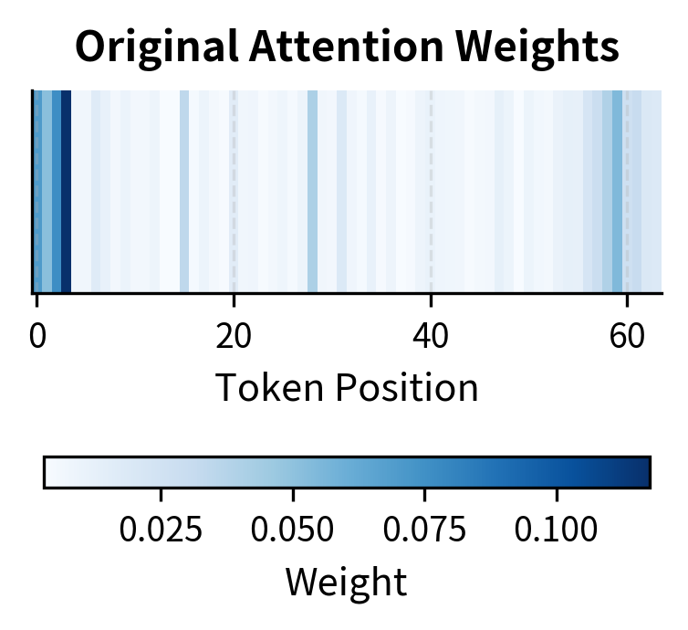
The key insight driving compression research is that not all cached tokens contribute equally to generation quality. Attention patterns in transformers are highly non-uniform: certain tokens receive concentrated attention while others are nearly ignored. This sparsity creates an opportunity. If we can identify and preserve the high-value cache entries while discarding the rest, we can dramatically reduce memory usage with minimal impact on output quality.

This chapter covers the three main approaches to KV cache compression: eviction-based strategies that remove entire token representations from the cache, attention sink preservation that protects critical initial tokens, and cache quantization that reduces the numerical precision of stored values. We'll examine the H2O (Heavy-Hitter Oracle) algorithm in detail as a representative eviction method, then explore how these techniques can be combined for maximum compression.

The Compression OpportunityLink Copied

Before diving into specific techniques, let's understand why compression is feasible in the first place. The fundamental question we need to answer is this: can we discard information from the KV cache without significantly harming generation quality? To answer this, consider the attention patterns in a typical language model generating the 500th token. The query for this new token computes attention scores against all 499 previous key vectors. In a perfectly uniform distribution, each previous token would receive $1/499 \approx 0.2\%$ of the attention. In practice, attention is far from uniform, and this non-uniformity is precisely what makes compression possible.

Studies of transformer attention patterns reveal several consistent phenomena that explain why some tokens matter far more than others:

Local focus: Recent tokens often receive disproportionate attention, especially in lower layers. This makes intuitive sense because language exhibits strong local coherence, with adjacent words often being grammatically and semantically related.
Anchor tokens: Certain semantically important tokens (subjects, verbs, key entities) attract attention regardless of distance. These tokens carry the core meaning of a passage and remain relevant throughout generation.
Attention sinks: As we covered in Part XV, initial tokens accumulate attention even when semantically irrelevant. This curious phenomenon appears to serve a computational purpose rather than a semantic one.
Sparse activation: Many tokens receive near-zero attention and contribute minimally to the output. These tokens are candidates for removal without significant quality degradation.

Out[2]:

Visualization

Bar chart showing attention weights across token positions with high weights at beginning, end, and two intermediate positions. — Simulated attention distribution showing characteristic non-uniformity. Initial tokens act as attention sinks, recent tokens receive local focus, and specific semantic positions (15, 28) act as anchor tokens. Many intermediate tokens receive near-zero attention, creating the compression opportunity.

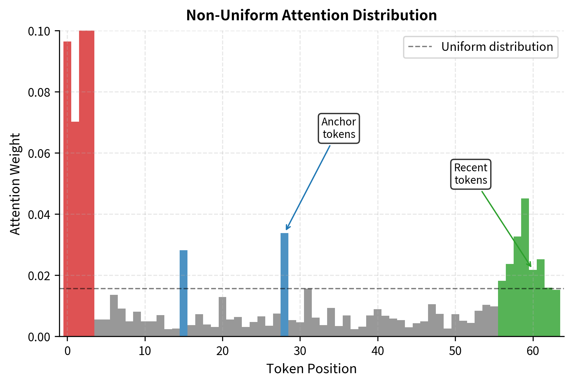
This non-uniformity means that a cache storing only the high-attention tokens might preserve most of the information needed for accurate generation. The attention distribution is not merely slightly skewed; it is often dramatically concentrated on a small subset of tokens. The challenge lies in identifying these important tokens efficiently, without requiring expensive computation at each generation step. We need methods that can predict which tokens will be important for future generation steps, not just which tokens have been important in the past.

Window-Based EvictionLink Copied

The simplest eviction strategy maintains a fixed-size sliding window, keeping only the most recent $k$ tokens in the cache. This approach has clear appeal for several reasons. It is trivial to implement, requires no analysis of attention patterns, and guarantees constant memory usage regardless of sequence length. The underlying assumption is that recent context is the most relevant context, which holds true for many language modeling scenarios.

In[3]:

Code

def sliding_window_cache(keys, values, window_size):
    """
    Maintains only the most recent window_size tokens in cache.

    Args:
        keys: (batch, heads, seq_len, head_dim)
        values: (batch, heads, seq_len, head_dim)
        window_size: Number of recent tokens to keep

    Returns:
        Truncated keys and values
    """
    seq_len = keys.size(2)

    if seq_len <= window_size:
        return keys, values

    # Keep only the last window_size tokens
    return keys[:, :, -window_size:, :], values[:, :, -window_size:, :]

def sliding_window_cache(keys, values, window_size):
    """
    Maintains only the most recent window_size tokens in cache.

    Args:
        keys: (batch, heads, seq_len, head_dim)
        values: (batch, heads, seq_len, head_dim)
        window_size: Number of recent tokens to keep

    Returns:
        Truncated keys and values
    """
    seq_len = keys.size(2)

    if seq_len <= window_size:
        return keys, values

    # Keep only the last window_size tokens
    return keys[:, :, -window_size:, :], values[:, :, -window_size:, :]

In[4]:

Code

import torch

# Demonstrate the sliding window
batch_size, num_heads, seq_len, head_dim = 1, 8, 100, 64
keys = torch.randn(batch_size, num_heads, seq_len, head_dim)
values = torch.randn(batch_size, num_heads, seq_len, head_dim)

window_size = 32
k_truncated, v_truncated = sliding_window_cache(keys, values, window_size)
memory_reduction_pct = (1 - window_size / seq_len) * 100

import torch

# Demonstrate the sliding window
batch_size, num_heads, seq_len, head_dim = 1, 8, 100, 64
keys = torch.randn(batch_size, num_heads, seq_len, head_dim)
values = torch.randn(batch_size, num_heads, seq_len, head_dim)

window_size = 32
k_truncated, v_truncated = sliding_window_cache(keys, values, window_size)
memory_reduction_pct = (1 - window_size / seq_len) * 100

Out[5]:

Console

Original cache: 100 tokens
Window size: 32
Truncated cache: 32 tokens
Memory reduction: 68.0%

Truncating to 32 tokens reduces cache memory by 68% in this example. The implementation is straightforward: we simply slice the tensor to keep only the final positions. However, this simplicity comes with a fundamental limitation: the approach discards all context beyond the window, including potentially crucial information from the beginning of the sequence.

Consider the practical implications through a concrete example. Imagine generating a response to a question. The question might appear at token positions 0-50, followed by supporting context at positions 51-400, with generation starting at position 401. A sliding window of 100 tokens would retain only tokens 301-400, losing the original question entirely. The model would have no memory of what it was asked, potentially producing irrelevant or incoherent responses. This illustrates why pure window-based approaches often fail for tasks requiring long-range dependencies. The approach works well for streaming applications or local language modeling, but breaks down when the task requires referencing distant context.

Attention-Based EvictionLink Copied

A more sophisticated approach selects tokens based on their historical attention scores rather than their recency. The intuition behind this method is straightforward: tokens that have received high attention in the past are likely to be important for future generation. These tokens have already proven their value, so preserving them makes sense. By tracking cumulative attention and evicting low-attention tokens, we can maintain a compact cache of the most relevant context while adapting to the specific content being processed.

The key insight here is that attention scores provide a signal of token importance. When the model attends heavily to a particular token, it extracts information from that token to inform its output. Tokens that consistently receive high attention across multiple generation steps are carrying information that the model repeatedly needs. These "frequently consulted" tokens are prime candidates for preservation, while tokens that receive negligible attention can likely be removed without consequence.

In[6]:

Code

import torch


class AttentionBasedCache:
    """
    Maintains a cache of fixed size by evicting tokens with lowest
    cumulative attention scores.
    """

    def __init__(self, max_cache_size, num_heads, head_dim):
        self.max_cache_size = max_cache_size
        self.num_heads = num_heads
        self.head_dim = head_dim

        # Initialize empty cache
        self.keys = None  # (batch, heads, cache_size, head_dim)
        self.values = None
        self.attention_scores = None  # Cumulative attention per token

    def update(self, new_key, new_value, attention_weights):
        """
        Add new token to cache and evict if necessary.

        Args:
            new_key: (batch, heads, 1, head_dim)
            new_value: (batch, heads, 1, head_dim)
            attention_weights: (batch, heads, 1, seq_len) - attention to all cached tokens
        """
        batch_size = new_key.size(0)

        if self.keys is None:
            # First token - initialize cache
            self.keys = new_key
            self.values = new_value
            # Initialize with the attention this token receives (from itself)
            self.attention_scores = attention_weights.mean(dim=1).squeeze(
                -2
            )  # (batch, 1)
            return

        # Append new token
        self.keys = torch.cat([self.keys, new_key], dim=2)
        self.values = torch.cat([self.values, new_value], dim=2)

        # Update cumulative attention scores for existing tokens
        # Average attention across heads, then add to cumulative scores
        current_attention = attention_weights.mean(dim=1).squeeze(
            -2
        )  # (batch, seq_len)

        # Existing tokens get their attention updated (all but last position)
        old_scores = self.attention_scores + current_attention[:, :-1]
        # New token starts with its self-attention score
        new_score = current_attention[:, -1:]

        self.attention_scores = torch.cat([old_scores, new_score], dim=1)

        # Evict if over capacity
        if self.keys.size(2) > self.max_cache_size:
            self._evict_lowest_attention()

    def _evict_lowest_attention(self):
        """Remove the token with lowest cumulative attention."""
        # Find index of minimum attention score
        _, min_idx = self.attention_scores.min(dim=1)

        batch_size = self.keys.size(0)

        # Create mask for tokens to keep (all except min_idx)
        keep_mask = torch.ones(batch_size, self.keys.size(2), dtype=torch.bool)
        for b in range(batch_size):
            keep_mask[b, min_idx[b]] = False

        # Apply mask
        # For simplicity, we'll handle batch_size=1 case
        self.keys = self.keys[:, :, keep_mask[0], :]
        self.values = self.values[:, :, keep_mask[0], :]
        self.attention_scores = self.attention_scores[:, keep_mask[0]]

import torch


class AttentionBasedCache:
    """
    Maintains a cache of fixed size by evicting tokens with lowest
    cumulative attention scores.
    """

    def __init__(self, max_cache_size, num_heads, head_dim):
        self.max_cache_size = max_cache_size
        self.num_heads = num_heads
        self.head_dim = head_dim

        # Initialize empty cache
        self.keys = None  # (batch, heads, cache_size, head_dim)
        self.values = None
        self.attention_scores = None  # Cumulative attention per token

    def update(self, new_key, new_value, attention_weights):
        """
        Add new token to cache and evict if necessary.

        Args:
            new_key: (batch, heads, 1, head_dim)
            new_value: (batch, heads, 1, head_dim)
            attention_weights: (batch, heads, 1, seq_len) - attention to all cached tokens
        """
        batch_size = new_key.size(0)

        if self.keys is None:
            # First token - initialize cache
            self.keys = new_key
            self.values = new_value
            # Initialize with the attention this token receives (from itself)
            self.attention_scores = attention_weights.mean(dim=1).squeeze(
                -2
            )  # (batch, 1)
            return

        # Append new token
        self.keys = torch.cat([self.keys, new_key], dim=2)
        self.values = torch.cat([self.values, new_value], dim=2)

        # Update cumulative attention scores for existing tokens
        # Average attention across heads, then add to cumulative scores
        current_attention = attention_weights.mean(dim=1).squeeze(
            -2
        )  # (batch, seq_len)

        # Existing tokens get their attention updated (all but last position)
        old_scores = self.attention_scores + current_attention[:, :-1]
        # New token starts with its self-attention score
        new_score = current_attention[:, -1:]

        self.attention_scores = torch.cat([old_scores, new_score], dim=1)

        # Evict if over capacity
        if self.keys.size(2) > self.max_cache_size:
            self._evict_lowest_attention()

    def _evict_lowest_attention(self):
        """Remove the token with lowest cumulative attention."""
        # Find index of minimum attention score
        _, min_idx = self.attention_scores.min(dim=1)

        batch_size = self.keys.size(0)

        # Create mask for tokens to keep (all except min_idx)
        keep_mask = torch.ones(batch_size, self.keys.size(2), dtype=torch.bool)
        for b in range(batch_size):
            keep_mask[b, min_idx[b]] = False

        # Apply mask
        # For simplicity, we'll handle batch_size=1 case
        self.keys = self.keys[:, :, keep_mask[0], :]
        self.values = self.values[:, :, keep_mask[0], :]
        self.attention_scores = self.attention_scores[:, keep_mask[0]]

This approach adapts dynamically to the content being processed. Important tokens accumulate high attention scores over time and remain in the cache, while less relevant tokens get evicted as their scores remain low. The method naturally identifies semantically meaningful tokens like subjects, key entities, and important verbs that the model needs to reference repeatedly.

However, the approach introduces computational overhead for tracking scores and, more critically, has a fundamental flaw that we must address. The flaw relates to a peculiar attention pattern we covered earlier: attention sinks. We will explore this issue and its solution in the next section.

Attention Sink PreservationLink Copied

As we discussed in Part XV, Chapter 5 on attention sinks, transformers exhibit a curious behavior that complicates attention-based eviction: initial tokens in a sequence accumulate disproportionate attention even when they carry no semantic importance. These "attention sinks" appear to serve as computational anchors, providing a stable target for attention heads to discharge probability mass when no relevant context exists. The phenomenon emerges from training dynamics: the model learns to use early tokens as a default attention target, creating a dependency that persists even when those tokens are semantically meaningless.

When we evict tokens based purely on historical attention scores, we risk removing these sink tokens because they may not have the highest cumulative attention. Counterintuitively, the initial tokens that receive high attention are not necessarily the tokens we should prioritize keeping based on semantic importance. The consequences of removing sinks can be severe. Without attention sinks available, models may produce incoherent outputs, fall into repetition loops, or exhibit generally degraded quality. The attention mechanism loses its computational anchor, disrupting the learned patterns that depend on its presence.

This creates a paradox for attention-based eviction strategies. The tokens receiving highest attention (the sinks) may not be semantically important, while truly important content tokens may receive only moderate attention because they share the attention budget with the sinks. Pure attention-score-based eviction conflates two distinct sources of high attention: semantic importance and computational anchoring.

The solution is elegantly simple: protect initial tokens from eviction regardless of their attention scores. By unconditionally preserving the first few tokens, we ensure the attention sinks remain available while still allowing the eviction policy to remove genuinely unimportant tokens from the rest of the sequence.

In[7]:

Code

import torch


class StreamingLLMCache:
    """
    Implements the StreamingLLM approach: preserve initial sink tokens
    plus a sliding window of recent tokens.

    Reference: "Efficient Streaming Language Models with Attention Sinks"
    """

    def __init__(self, sink_size, window_size, num_heads, head_dim):
        self.sink_size = sink_size  # Number of initial tokens to always keep
        self.window_size = window_size  # Number of recent tokens to keep
        self.num_heads = num_heads
        self.head_dim = head_dim

        self.keys = None
        self.values = None
        self.total_tokens_seen = 0

    @property
    def max_cache_size(self):
        return self.sink_size + self.window_size

    def update(self, new_key, new_value):
        """
        Add new token, maintaining sink tokens and recent window.

        Args:
            new_key: (batch, heads, 1, head_dim)
            new_value: (batch, heads, 1, head_dim)
        """
        self.total_tokens_seen += 1

        if self.keys is None:
            self.keys = new_key
            self.values = new_value
            return

        # Append new token
        self.keys = torch.cat([self.keys, new_key], dim=2)
        self.values = torch.cat([self.values, new_value], dim=2)

        current_size = self.keys.size(2)

        # If we exceed capacity, keep sinks + recent window
        if current_size > self.max_cache_size:
            # Keep first sink_size tokens and last window_size tokens
            sink_keys = self.keys[:, :, : self.sink_size, :]
            sink_values = self.values[:, :, : self.sink_size, :]

            window_keys = self.keys[:, :, -self.window_size :, :]
            window_values = self.values[:, :, -self.window_size :, :]

            self.keys = torch.cat([sink_keys, window_keys], dim=2)
            self.values = torch.cat([sink_values, window_values], dim=2)

    def get_cache(self):
        """Return current key-value cache."""
        return self.keys, self.values

import torch


class StreamingLLMCache:
    """
    Implements the StreamingLLM approach: preserve initial sink tokens
    plus a sliding window of recent tokens.

    Reference: "Efficient Streaming Language Models with Attention Sinks"
    """

    def __init__(self, sink_size, window_size, num_heads, head_dim):
        self.sink_size = sink_size  # Number of initial tokens to always keep
        self.window_size = window_size  # Number of recent tokens to keep
        self.num_heads = num_heads
        self.head_dim = head_dim

        self.keys = None
        self.values = None
        self.total_tokens_seen = 0

    @property
    def max_cache_size(self):
        return self.sink_size + self.window_size

    def update(self, new_key, new_value):
        """
        Add new token, maintaining sink tokens and recent window.

        Args:
            new_key: (batch, heads, 1, head_dim)
            new_value: (batch, heads, 1, head_dim)
        """
        self.total_tokens_seen += 1

        if self.keys is None:
            self.keys = new_key
            self.values = new_value
            return

        # Append new token
        self.keys = torch.cat([self.keys, new_key], dim=2)
        self.values = torch.cat([self.values, new_value], dim=2)

        current_size = self.keys.size(2)

        # If we exceed capacity, keep sinks + recent window
        if current_size > self.max_cache_size:
            # Keep first sink_size tokens and last window_size tokens
            sink_keys = self.keys[:, :, : self.sink_size, :]
            sink_values = self.values[:, :, : self.sink_size, :]

            window_keys = self.keys[:, :, -self.window_size :, :]
            window_values = self.values[:, :, -self.window_size :, :]

            self.keys = torch.cat([sink_keys, window_keys], dim=2)
            self.values = torch.cat([sink_values, window_values], dim=2)

    def get_cache(self):
        """Return current key-value cache."""
        return self.keys, self.values

In[8]:

Code

import torch


# Demonstrate StreamingLLM cache behavior
def simulate_generation(cache, num_tokens):
    """Simulate generating num_tokens and track cache state."""
    batch_size = 1

    history = []
    for i in range(num_tokens):
        # Simulate a new key-value pair
        new_key = torch.randn(batch_size, cache.num_heads, 1, cache.head_dim)
        new_value = torch.randn(batch_size, cache.num_heads, 1, cache.head_dim)

        cache.update(new_key, new_value)

        if cache.keys is not None:
            history.append(cache.keys.size(2))

    return history

import torch


# Demonstrate StreamingLLM cache behavior
def simulate_generation(cache, num_tokens):
    """Simulate generating num_tokens and track cache state."""
    batch_size = 1

    history = []
    for i in range(num_tokens):
        # Simulate a new key-value pair
        new_key = torch.randn(batch_size, cache.num_heads, 1, cache.head_dim)
        new_value = torch.randn(batch_size, cache.num_heads, 1, cache.head_dim)

        cache.update(new_key, new_value)

        if cache.keys is not None:
            history.append(cache.keys.size(2))

    return history

In[9]:

Code

cache = StreamingLLMCache(sink_size=4, window_size=32, num_heads=8, head_dim=64)
history = simulate_generation(cache, 100)

cache = StreamingLLMCache(sink_size=4, window_size=32, num_heads=8, head_dim=64)
history = simulate_generation(cache, 100)

Out[10]:

Console

Configuration: 4 sink tokens + 32 window
Maximum cache size: 36 tokens

Cache size over generation:
  After 10 tokens: 10
  After 36 tokens: 36
  After 50 tokens: 36
  After 100 tokens: 36

The StreamingLLM approach maintains exactly sink_size + window_size tokens once the cache is full, providing predictable memory usage while preserving the critical attention sinks. The cache size grows linearly during the initial phase, then plateaus at the maximum size and remains constant regardless of how many additional tokens are generated. This bounded memory behavior enables indefinitely long streaming generation.

Out[11]:

Visualization

Line plot comparing cache sizes over generation steps for different eviction strategies. — Cache size comparison between StreamingLLM and sliding window approaches over 100 generated tokens. StreamingLLM (sink + window) maintains bounded memory after reaching capacity, while a hypothetical unbounded cache would grow linearly. Both approaches plateau, but StreamingLLM preserves critical initial tokens.

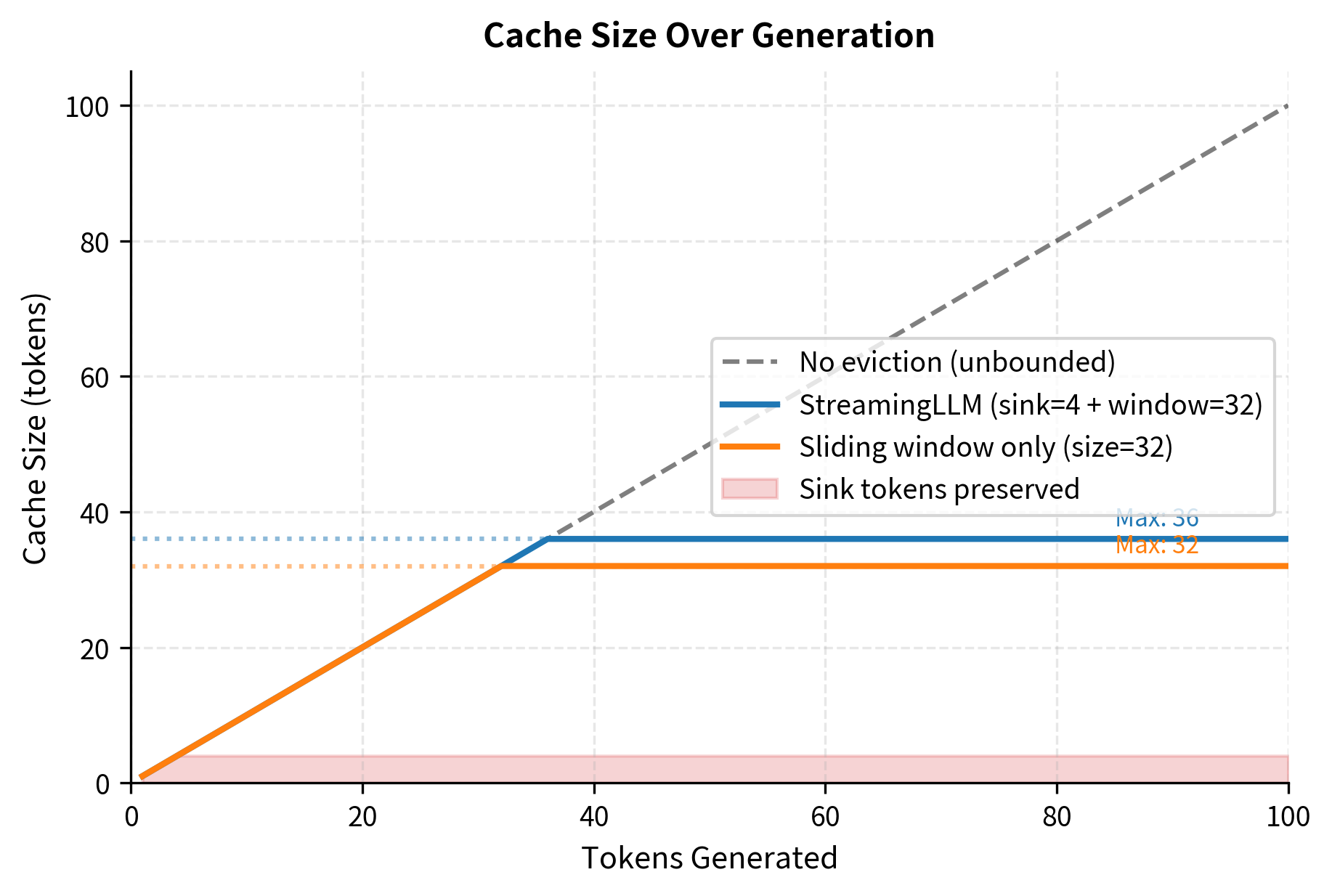
Research has shown that just 4 sink tokens are typically sufficient to maintain generation quality, making this a highly efficient solution. The small sink budget adds minimal memory overhead while providing the computational anchoring the model requires. Combined with a modest window size, the approach achieves substantial compression while maintaining coherent generation for streaming applications.

The H2O AlgorithmLink Copied

Heavy-Hitter Oracle (H2O) represents a more sophisticated eviction policy that extends beyond simple recency or sink preservation. The algorithm combines attention-based selection with sink preservation, addressing the limitations of both pure window-based and pure attention-based approaches. The key insight motivating H2O is that tokens exhibit different temporal importance patterns. Some tokens are "heavy hitters," consistently receiving high attention across many generation steps because they carry information the model repeatedly needs. Other tokens are transient, relevant only briefly before becoming obsolete as generation proceeds.

Consider how these patterns manifest in practice. A subject noun at the beginning of a paragraph might be a heavy hitter, receiving attention throughout the paragraph as the model maintains coherence. A transition word, by contrast, might receive attention only from the immediately following tokens before becoming irrelevant. H2O captures this distinction by tracking cumulative attention over time and using it to identify tokens worthy of long-term preservation.

H2O maintains two categories of tokens that serve complementary purposes:

Recent tokens: A sliding window of the most recent $k_{\text{recent}}$ tokens. These provide immediate local context and ensure the model can maintain coherent generation based on what was just produced.
Heavy hitters: Tokens with the highest cumulative attention scores, capped at $k_{\text{heavy}}$ tokens. These represent semantically important content that the model has repeatedly consulted, suggesting continued relevance.

The algorithm dynamically balances these sets throughout generation, ensuring that both recency and historical importance are considered when making eviction decisions. Tokens can transition between categories: a recent token that accumulates high attention becomes a heavy hitter candidate, while a former heavy hitter that stops receiving attention may eventually be evicted.

In[12]:

Code

import torch


class H2OCache:
    """
    Heavy-Hitter Oracle (H2O) KV cache compression.

    Maintains recent tokens plus heavy-hitters (tokens with highest
    cumulative attention scores).

    Reference: "H2O: Heavy-Hitter Oracle for Efficient Generative Inference"
    """

    def __init__(self, recent_size, heavy_hitter_size, num_heads, head_dim):
        self.recent_size = recent_size
        self.heavy_hitter_size = heavy_hitter_size
        self.num_heads = num_heads
        self.head_dim = head_dim

        # Cache storage
        self.keys = None  # (batch, heads, cache_size, head_dim)
        self.values = None
        self.cumulative_attention = None  # (batch, cache_size)
        self.token_positions = None  # Original position of each token

    @property
    def max_cache_size(self):
        return self.recent_size + self.heavy_hitter_size

    def update(self, new_key, new_value, attention_weights):
        """
        Add new token and update heavy-hitter statistics.

        Args:
            new_key: (batch, heads, 1, head_dim)
            new_value: (batch, heads, 1, head_dim)
            attention_weights: (batch, heads, 1, current_cache_size)
        """
        batch_size = new_key.size(0)

        if self.keys is None:
            # Initialize with first token
            self.keys = new_key
            self.values = new_value
            self.cumulative_attention = torch.zeros(batch_size, 1)
            self.token_positions = torch.tensor([[0]])
            return

        # Update cumulative attention for existing tokens
        # Average across heads for simplicity
        attn_update = attention_weights.mean(dim=1).squeeze(
            -2
        )  # (batch, cache_size)
        self.cumulative_attention = self.cumulative_attention + attn_update

        # Add new token
        new_position = self.token_positions.max() + 1
        self.keys = torch.cat([self.keys, new_key], dim=2)
        self.values = torch.cat([self.values, new_value], dim=2)
        self.cumulative_attention = torch.cat(
            [self.cumulative_attention, torch.zeros(batch_size, 1)], dim=1
        )
        self.token_positions = torch.cat(
            [self.token_positions, torch.tensor([[new_position]])], dim=1
        )

        # Evict if necessary
        current_size = self.keys.size(2)
        if current_size > self.max_cache_size:
            self._evict()

    def _evict(self):
        """
        Evict tokens to maintain cache size.
        Keep: recent_size most recent + heavy_hitter_size highest attention
        """
        batch_size = self.keys.size(0)
        current_size = self.keys.size(2)

        # Identify recent tokens (by position)
        positions = self.token_positions[0]  # (cache_size,)
        _, recent_indices = positions.topk(self.recent_size)
        recent_mask = torch.zeros(current_size, dtype=torch.bool)
        recent_mask[recent_indices] = True

        # Among non-recent tokens, find heavy hitters
        non_recent_mask = ~recent_mask
        non_recent_attention = self.cumulative_attention[0].clone()
        non_recent_attention[recent_mask] = float("-inf")  # Exclude recent

        # Get top heavy hitters from non-recent tokens
        _, heavy_hitter_indices = non_recent_attention.topk(
            min(self.heavy_hitter_size, non_recent_mask.sum())
        )
        heavy_hitter_mask = torch.zeros(current_size, dtype=torch.bool)
        heavy_hitter_mask[heavy_hitter_indices] = True

        # Keep tokens that are either recent or heavy hitters
        keep_mask = recent_mask | heavy_hitter_mask

        # Apply mask
        self.keys = self.keys[:, :, keep_mask, :]
        self.values = self.values[:, :, keep_mask, :]
        self.cumulative_attention = self.cumulative_attention[:, keep_mask]
        self.token_positions = self.token_positions[:, keep_mask]

import torch


class H2OCache:
    """
    Heavy-Hitter Oracle (H2O) KV cache compression.

    Maintains recent tokens plus heavy-hitters (tokens with highest
    cumulative attention scores).

    Reference: "H2O: Heavy-Hitter Oracle for Efficient Generative Inference"
    """

    def __init__(self, recent_size, heavy_hitter_size, num_heads, head_dim):
        self.recent_size = recent_size
        self.heavy_hitter_size = heavy_hitter_size
        self.num_heads = num_heads
        self.head_dim = head_dim

        # Cache storage
        self.keys = None  # (batch, heads, cache_size, head_dim)
        self.values = None
        self.cumulative_attention = None  # (batch, cache_size)
        self.token_positions = None  # Original position of each token

    @property
    def max_cache_size(self):
        return self.recent_size + self.heavy_hitter_size

    def update(self, new_key, new_value, attention_weights):
        """
        Add new token and update heavy-hitter statistics.

        Args:
            new_key: (batch, heads, 1, head_dim)
            new_value: (batch, heads, 1, head_dim)
            attention_weights: (batch, heads, 1, current_cache_size)
        """
        batch_size = new_key.size(0)

        if self.keys is None:
            # Initialize with first token
            self.keys = new_key
            self.values = new_value
            self.cumulative_attention = torch.zeros(batch_size, 1)
            self.token_positions = torch.tensor([[0]])
            return

        # Update cumulative attention for existing tokens
        # Average across heads for simplicity
        attn_update = attention_weights.mean(dim=1).squeeze(
            -2
        )  # (batch, cache_size)
        self.cumulative_attention = self.cumulative_attention + attn_update

        # Add new token
        new_position = self.token_positions.max() + 1
        self.keys = torch.cat([self.keys, new_key], dim=2)
        self.values = torch.cat([self.values, new_value], dim=2)
        self.cumulative_attention = torch.cat(
            [self.cumulative_attention, torch.zeros(batch_size, 1)], dim=1
        )
        self.token_positions = torch.cat(
            [self.token_positions, torch.tensor([[new_position]])], dim=1
        )

        # Evict if necessary
        current_size = self.keys.size(2)
        if current_size > self.max_cache_size:
            self._evict()

    def _evict(self):
        """
        Evict tokens to maintain cache size.
        Keep: recent_size most recent + heavy_hitter_size highest attention
        """
        batch_size = self.keys.size(0)
        current_size = self.keys.size(2)

        # Identify recent tokens (by position)
        positions = self.token_positions[0]  # (cache_size,)
        _, recent_indices = positions.topk(self.recent_size)
        recent_mask = torch.zeros(current_size, dtype=torch.bool)
        recent_mask[recent_indices] = True

        # Among non-recent tokens, find heavy hitters
        non_recent_mask = ~recent_mask
        non_recent_attention = self.cumulative_attention[0].clone()
        non_recent_attention[recent_mask] = float("-inf")  # Exclude recent

        # Get top heavy hitters from non-recent tokens
        _, heavy_hitter_indices = non_recent_attention.topk(
            min(self.heavy_hitter_size, non_recent_mask.sum())
        )
        heavy_hitter_mask = torch.zeros(current_size, dtype=torch.bool)
        heavy_hitter_mask[heavy_hitter_indices] = True

        # Keep tokens that are either recent or heavy hitters
        keep_mask = recent_mask | heavy_hitter_mask

        # Apply mask
        self.keys = self.keys[:, :, keep_mask, :]
        self.values = self.values[:, :, keep_mask, :]
        self.cumulative_attention = self.cumulative_attention[:, keep_mask]
        self.token_positions = self.token_positions[:, keep_mask]

In[13]:

Code

import torch
import torch.nn.functional as F


def demonstrate_h2o(heavy_hitter_positions):
    """Show H2O cache behavior with varying attention patterns."""
    batch_size = 1
    num_heads = 8
    head_dim = 64

    cache = H2OCache(
        recent_size=8,
        heavy_hitter_size=8,
        num_heads=num_heads,
        head_dim=head_dim,
    )

    # Simulate 50 tokens with varying attention patterns
    for t in range(50):
        new_key = torch.randn(batch_size, num_heads, 1, head_dim)
        new_value = torch.randn(batch_size, num_heads, 1, head_dim)

        if cache.keys is not None:
            current_size = cache.keys.size(2)
            # Create attention weights
            attn = torch.rand(batch_size, num_heads, 1, current_size)

            # Give extra attention to heavy hitter positions if they're in cache
            for pos_idx, pos in enumerate(cache.token_positions[0].tolist()):
                if pos in heavy_hitter_positions:
                    attn[:, :, :, pos_idx] += 2.0  # Boost attention

            # Normalize
            attn = F.softmax(attn, dim=-1)
            cache.update(new_key, new_value, attn)
        else:
            cache.update(new_key, new_value, None)

    return cache

import torch
import torch.nn.functional as F


def demonstrate_h2o(heavy_hitter_positions):
    """Show H2O cache behavior with varying attention patterns."""
    batch_size = 1
    num_heads = 8
    head_dim = 64

    cache = H2OCache(
        recent_size=8,
        heavy_hitter_size=8,
        num_heads=num_heads,
        head_dim=head_dim,
    )

    # Simulate 50 tokens with varying attention patterns
    for t in range(50):
        new_key = torch.randn(batch_size, num_heads, 1, head_dim)
        new_value = torch.randn(batch_size, num_heads, 1, head_dim)

        if cache.keys is not None:
            current_size = cache.keys.size(2)
            # Create attention weights
            attn = torch.rand(batch_size, num_heads, 1, current_size)

            # Give extra attention to heavy hitter positions if they're in cache
            for pos_idx, pos in enumerate(cache.token_positions[0].tolist()):
                if pos in heavy_hitter_positions:
                    attn[:, :, :, pos_idx] += 2.0  # Boost attention

            # Normalize
            attn = F.softmax(attn, dim=-1)
            cache.update(new_key, new_value, attn)
        else:
            cache.update(new_key, new_value, None)

    return cache

In[14]:

Code

heavy_hitter_positions = {5, 10}
cache = demonstrate_h2o(heavy_hitter_positions)

heavy_hitter_positions = {5, 10}
cache = demonstrate_h2o(heavy_hitter_positions)

Out[15]:

Console

After 50 tokens:
  Cache size: 16 tokens
  Token positions in cache: [0, 1, 2, 3, 4, 5, 6, 10, 42, 43, 44, 45, 46, 47, 48, 49]

Cumulative attention scores:
  Position  0: 4.009
  Position  1: 3.053
  Position  2: 2.600
  Position  3: 2.247
  Position  4: 1.945
  Position  5: 12.489 (heavy hitter)
  Position  6: 1.711
  Position 10: 9.881 (heavy hitter)
  Position 42: 0.238
  Position 43: 0.210
  Position 44: 0.177
  Position 45: 0.148
  Position 46: 0.096
  Position 47: 0.072
  Position 48: 0.033
  Position 49: 0.000

Notice how positions 5 and 10 are retained in the cache despite not being among the most recent tokens. Their high cumulative attention scores qualify them as heavy hitters, preserving important context while still maintaining recency through the recent token budget. The algorithm has automatically identified these tokens as carrying important information that the model repeatedly needs, and it protects them from eviction even as dozens of newer tokens have been generated.

Out[16]:

Visualization

Bar chart showing cumulative attention scores for retained tokens with heavy hitters and recent tokens color-coded. — H2O cache composition showing token categorization and retention based on cumulative attention. Heavy hitters at positions 5 and 10 are preserved despite distance, while the most recent tokens form a sliding window to maintain local context. This dual strategy ensures both semantic importance and recency are represented.

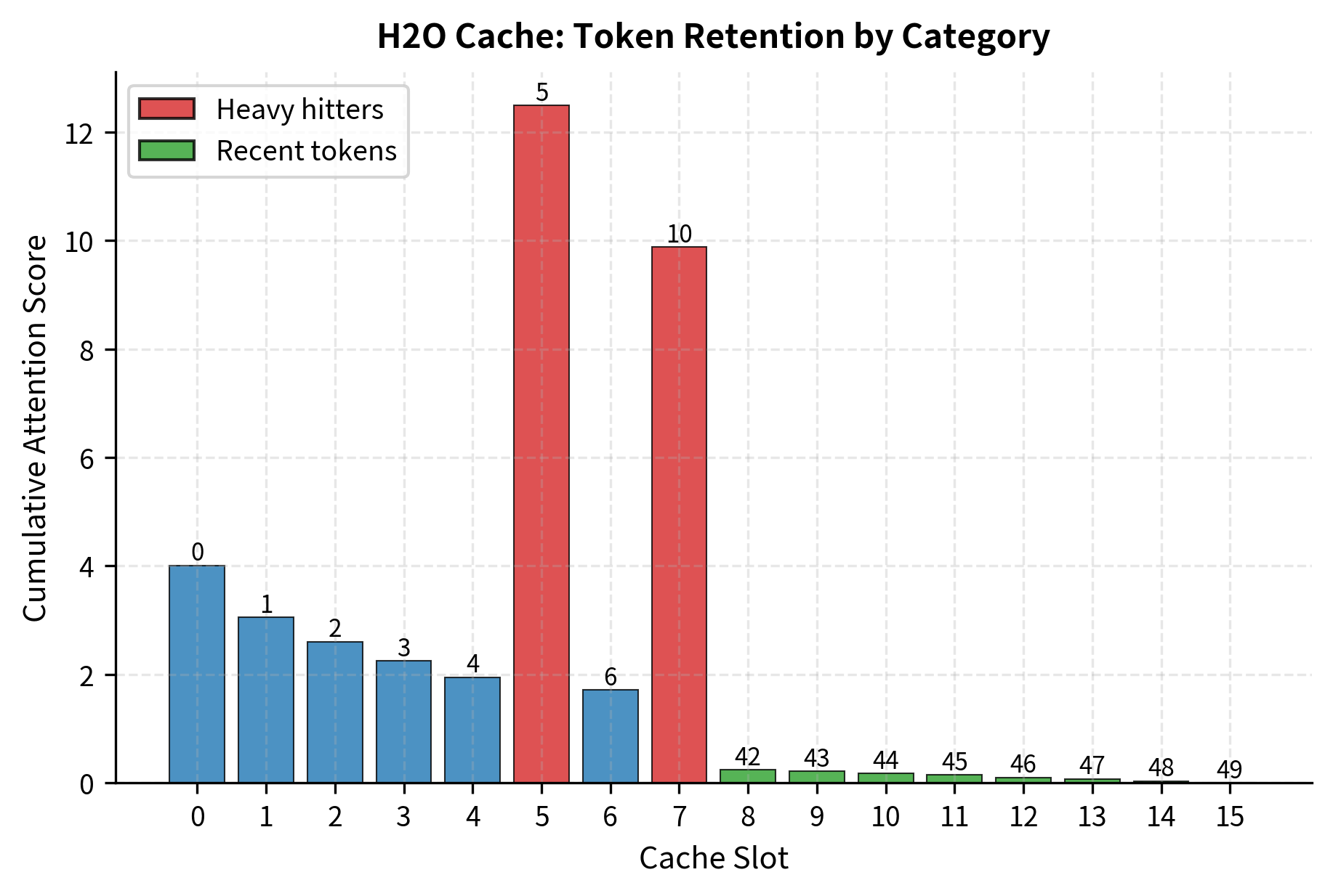
The cumulative attention scores reveal the distinction between heavy hitters and ordinary tokens. Positions 5 and 10 have accumulated substantially higher scores than other retained positions because the simulated attention pattern consistently attended to them. In a real model, these high-attention tokens would typically correspond to semantically important content: the subject of a sentence, a key entity being discussed, or a critical fact that informs subsequent generation.

Cache QuantizationLink Copied

Orthogonal to eviction strategies, cache quantization reduces memory by storing key and value vectors at lower numerical precision. While model weights typically use FP16 or BF16 during inference, the cached activations can often tolerate even lower precision without significant quality loss. This approach complements eviction: rather than removing tokens entirely, we keep all tokens but represent each one using fewer bits.

The mathematical foundation of quantization is straightforward. We need to map continuous floating-point values to a discrete set of integers that can be stored compactly. The simplest form is uniform quantization which divides the value range into equally-spaced bins and maps each floating-point value to the nearest bin:

q = \text{round}\left(\frac{x - x_{\min}}{x_{\max} - x_{\min}} \cdot (2^b - 1)\right)

Let us carefully examine each component of this formula to understand how it accomplishes the mapping from floating-point to integer representation:

$q$ : the resulting quantized integer index, which will be stored in place of the original floating-point value
$x$ : the original floating-point value that we wish to compress
$x_{\min}$ : the minimum value in the group being quantized, establishing the lower bound of the value range
$x_{\max}$ : the maximum value in the group being quantized, establishing the upper bound of the value range
$b$ : the target bit width (e.g., 8 for INT8 or 4 for INT4), determining how many discrete levels are available
$2^b - 1$ : the total number of discrete quantization levels, which equals the maximum integer value representable

This transformation accomplishes its goal through a sequence of intuitive steps. First, it normalizes the original value $x$ to the range $[0, 1]$ by computing the fraction $\frac{x - x_{\min}}{x_{\max} - x_{\min}}$ . This fraction represents where $x$ falls within the overall range of values. Second, it scales this normalized value to the full integer range $[0, 2^b - 1]$ by multiplication. Finally, it rounds to the nearest integer to obtain a discrete representation that can be stored efficiently. This approach preserves the relative ordering and approximate magnitudes of values while dramatically reducing storage requirements.

When we need to use the cached values for computation, we must reverse this process. Dequantization recovers an approximation of the original value:

\hat{x} = \frac{q}{2^b - 1} \cdot (x_{\max} - x_{\min}) + x_{\min}

Again, let us examine each component to understand the reconstruction process:

$\hat{x}$ : the reconstructed floating-point value, which approximates the original $x$
$q$ : the stored quantized integer retrieved from memory
$b$ : the target bit width used during quantization
$x_{\min}$ : the minimum value from the original group, serving as the offset that restores the correct baseline
$x_{\max} - x_{\min}$ : the dynamic range of the original values, used to restore the correct magnitude

The reconstruction process precisely reverses the quantization steps. It first converts the integer $q$ back to a proportion in $[0, 1]$ by dividing by the maximum integer value. It then maps that proportion onto the original dynamic range by multiplying by $(x_{\max} - x_{\min})$ . Finally, it adds the offset $x_{\min}$ to restore the correct baseline. The reconstructed value $\hat{x}$ will differ from the original $x$ by at most half a quantization step, introducing a small but bounded error.

In[17]:

Code

import torch


class QuantizedCache:
    """
    KV cache with quantized storage.
    Stores keys and values at reduced precision.
    """

    def __init__(self, bits=8):
        self.bits = bits
        self.max_val = 2**bits - 1

        # Quantized storage
        self.keys_quantized = None
        self.values_quantized = None

        # Quantization parameters (per-tensor)
        self.key_min = None
        self.key_scale = None
        self.value_min = None
        self.value_scale = None

    def quantize(self, tensor):
        """Quantize tensor to self.bits precision."""
        t_min = tensor.min()
        t_max = tensor.max()
        scale = (t_max - t_min) / self.max_val

        # Avoid division by zero
        if scale == 0:
            scale = torch.tensor(1.0)

        quantized = torch.round((tensor - t_min) / scale).to(torch.uint8)
        return quantized, t_min, scale

    def dequantize(self, quantized, t_min, scale):
        """Recover approximate float tensor."""
        return quantized.float() * scale + t_min

    def store(self, keys, values):
        """Store key-value pairs in quantized format."""
        self.keys_quantized, self.key_min, self.key_scale = self.quantize(keys)
        self.values_quantized, self.value_min, self.value_scale = self.quantize(
            values
        )

    def retrieve(self):
        """Retrieve dequantized key-value pairs."""
        keys = self.dequantize(
            self.keys_quantized, self.key_min, self.key_scale
        )
        values = self.dequantize(
            self.values_quantized, self.value_min, self.value_scale
        )
        return keys, values

    def memory_usage(self, original_dtype=torch.float16):
        """Compare memory usage."""
        if self.keys_quantized is None:
            return 0, 0

        # Quantized: uint8 = 1 byte per element
        quantized_bytes = (
            self.keys_quantized.numel() + self.values_quantized.numel()
        )

        # Original: 2 bytes for FP16
        original_bytes = (
            self.keys_quantized.numel() + self.values_quantized.numel()
        ) * 2

        return quantized_bytes, original_bytes

import torch


class QuantizedCache:
    """
    KV cache with quantized storage.
    Stores keys and values at reduced precision.
    """

    def __init__(self, bits=8):
        self.bits = bits
        self.max_val = 2**bits - 1

        # Quantized storage
        self.keys_quantized = None
        self.values_quantized = None

        # Quantization parameters (per-tensor)
        self.key_min = None
        self.key_scale = None
        self.value_min = None
        self.value_scale = None

    def quantize(self, tensor):
        """Quantize tensor to self.bits precision."""
        t_min = tensor.min()
        t_max = tensor.max()
        scale = (t_max - t_min) / self.max_val

        # Avoid division by zero
        if scale == 0:
            scale = torch.tensor(1.0)

        quantized = torch.round((tensor - t_min) / scale).to(torch.uint8)
        return quantized, t_min, scale

    def dequantize(self, quantized, t_min, scale):
        """Recover approximate float tensor."""
        return quantized.float() * scale + t_min

    def store(self, keys, values):
        """Store key-value pairs in quantized format."""
        self.keys_quantized, self.key_min, self.key_scale = self.quantize(keys)
        self.values_quantized, self.value_min, self.value_scale = self.quantize(
            values
        )

    def retrieve(self):
        """Retrieve dequantized key-value pairs."""
        keys = self.dequantize(
            self.keys_quantized, self.key_min, self.key_scale
        )
        values = self.dequantize(
            self.values_quantized, self.value_min, self.value_scale
        )
        return keys, values

    def memory_usage(self, original_dtype=torch.float16):
        """Compare memory usage."""
        if self.keys_quantized is None:
            return 0, 0

        # Quantized: uint8 = 1 byte per element
        quantized_bytes = (
            self.keys_quantized.numel() + self.values_quantized.numel()
        )

        # Original: 2 bytes for FP16
        original_bytes = (
            self.keys_quantized.numel() + self.values_quantized.numel()
        ) * 2

        return quantized_bytes, original_bytes

In[18]:

Code

import torch.nn.functional as F


def evaluate_quantization_error(keys, values, bits_list=[8, 4, 2]):
    """Measure reconstruction error at different bit widths."""
    results = []

    for bits in bits_list:
        cache = QuantizedCache(bits=bits)
        cache.store(keys, values)

        keys_recovered, values_recovered = cache.retrieve()

        # Compute mean squared error
        key_mse = F.mse_loss(keys_recovered, keys).item()
        value_mse = F.mse_loss(values_recovered, values).item()

        # Compute cosine similarity (important for attention)
        key_cos = F.cosine_similarity(
            keys.flatten(), keys_recovered.flatten(), dim=0
        ).item()

        quant_bytes, orig_bytes = cache.memory_usage()

        results.append(
            {
                "bits": bits,
                "key_mse": key_mse,
                "value_mse": value_mse,
                "key_cosine_sim": key_cos,
                "compression_ratio": orig_bytes / quant_bytes
                if quant_bytes > 0
                else 0,
            }
        )

    return results

import torch.nn.functional as F


def evaluate_quantization_error(keys, values, bits_list=[8, 4, 2]):
    """Measure reconstruction error at different bit widths."""
    results = []

    for bits in bits_list:
        cache = QuantizedCache(bits=bits)
        cache.store(keys, values)

        keys_recovered, values_recovered = cache.retrieve()

        # Compute mean squared error
        key_mse = F.mse_loss(keys_recovered, keys).item()
        value_mse = F.mse_loss(values_recovered, values).item()

        # Compute cosine similarity (important for attention)
        key_cos = F.cosine_similarity(
            keys.flatten(), keys_recovered.flatten(), dim=0
        ).item()

        quant_bytes, orig_bytes = cache.memory_usage()

        results.append(
            {
                "bits": bits,
                "key_mse": key_mse,
                "value_mse": value_mse,
                "key_cosine_sim": key_cos,
                "compression_ratio": orig_bytes / quant_bytes
                if quant_bytes > 0
                else 0,
            }
        )

    return results

In[19]:

Code

import torch

## Test with realistic cache data
batch_size, num_heads, seq_len, head_dim = 1, 32, 512, 128
keys = torch.randn(batch_size, num_heads, seq_len, head_dim)
values = torch.randn(batch_size, num_heads, seq_len, head_dim)

results = evaluate_quantization_error(keys, values, bits_list=[8, 4, 2])

import torch

## Test with realistic cache data
batch_size, num_heads, seq_len, head_dim = 1, 32, 512, 128
keys = torch.randn(batch_size, num_heads, seq_len, head_dim)
values = torch.randn(batch_size, num_heads, seq_len, head_dim)

results = evaluate_quantization_error(keys, values, bits_list=[8, 4, 2])

Out[20]:

Console

Quantization Analysis:
-----------------------------------------------------------------
  Bits      Key MSE    Value MSE   Key Cosine  Compression
-----------------------------------------------------------------
     8     0.000130     0.000114       1.0001         2.0x
     4     0.037668     0.033059       0.9817         2.0x
     2     1.133774     0.961849       0.7967         2.0x

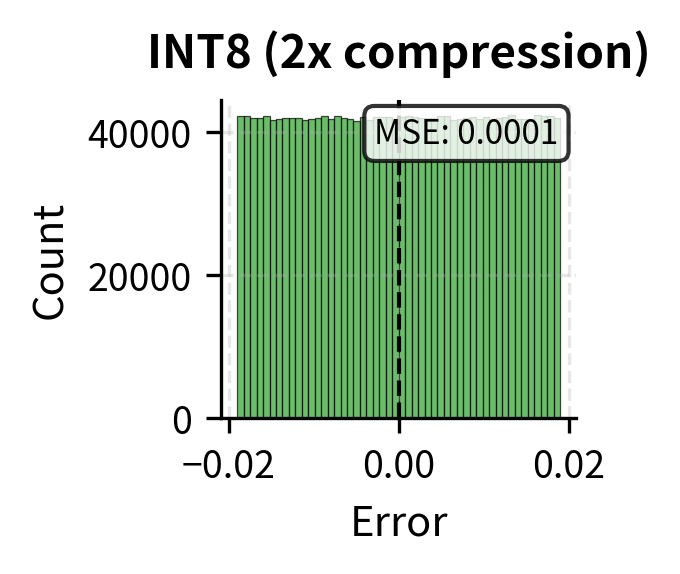
INT8 quantization achieves 2x compression with minimal error, maintaining cosine similarity above 0.99. This high cosine similarity is particularly important because attention operates on dot products between queries and keys. The dot product is fundamentally a measure of similarity, and if the quantized keys preserve high cosine similarity with their original values, the resulting attention scores will be nearly identical to what they would have been without quantization.

Out[21]:

Visualization

Three histograms showing error distributions becoming wider as bit width decreases from 8 to 4 to 2 bits. — Quantization error distribution across varying bit widths, computed as the element-wise difference between original and reconstructed values. Accuracy degrades as precision decreases: INT8 shows minimal error, while INT2 exhibits substantial spread that can impair attention. The plots demonstrate the trade-off between compression ratio and numerical fidelity.

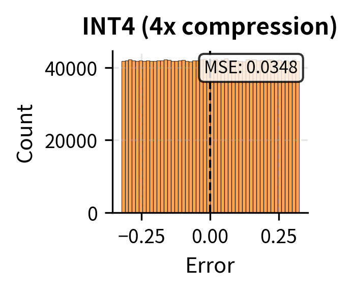
Even INT4 quantization, which provides 4x compression, often preserves sufficient similarity for acceptable generation quality. However, quality degradation becomes noticeable for precision-sensitive tasks at this level. The trade-off between compression and accuracy depends heavily on the specific application: chat applications may tolerate INT4 well, while code generation or mathematical reasoning may require the precision of INT8 or higher.

Per-Channel QuantizationLink Copied

The per-tensor quantization approach we examined computes global statistics across the entire tensor, using a single minimum and scale value for all elements. This approach is simple but can be suboptimal when different attention heads or dimensions have varying value ranges. If one head has values concentrated in a narrow range while another has a wide range, using global statistics forces the narrow-range head to use only a fraction of the available quantization levels, wasting precision.

Per-channel quantization improves accuracy by computing separate scales for each head or channel. Each attention head gets its own minimum and scale values, allowing it to use the full range of quantization levels regardless of what other heads are doing. This independence is particularly valuable because different attention heads often specialize in different types of patterns and may exhibit quite different value distributions.

In[22]:

Code

import torch


class PerChannelQuantizedCache:
    """
    KV cache with per-head quantization for better accuracy.
    """

    def __init__(self, bits=8):
        self.bits = bits
        self.max_val = 2**bits - 1

        self.keys_quantized = None
        self.values_quantized = None
        self.key_params = None  # (min, scale) per head
        self.value_params = None

    def quantize_per_head(self, tensor):
        """
        Quantize with separate parameters per attention head.
        tensor shape: (batch, heads, seq_len, head_dim)
        """
        batch_size, num_heads, seq_len, head_dim = tensor.shape

        # Compute min/max per head
        # Reshape to (batch * heads, seq_len * head_dim) for per-head stats
        reshaped = tensor.view(batch_size * num_heads, -1)
        t_min = reshaped.min(dim=1, keepdim=True)[0]
        t_max = reshaped.max(dim=1, keepdim=True)[0]

        scale = (t_max - t_min) / self.max_val
        scale = torch.where(scale == 0, torch.ones_like(scale), scale)

        # Quantize
        quantized = torch.round((reshaped - t_min) / scale)
        quantized = quantized.clamp(0, self.max_val).to(torch.uint8)
        quantized = quantized.view(batch_size, num_heads, seq_len, head_dim)

        return quantized, (t_min, scale)

    def dequantize_per_head(self, quantized, params):
        """Dequantize using per-head parameters."""
        t_min, scale = params
        batch_size, num_heads, seq_len, head_dim = quantized.shape

        reshaped = quantized.view(batch_size * num_heads, -1).float()
        dequantized = reshaped * scale + t_min

        return dequantized.view(batch_size, num_heads, seq_len, head_dim)

    def store(self, keys, values):
        self.keys_quantized, self.key_params = self.quantize_per_head(keys)
        self.values_quantized, self.value_params = self.quantize_per_head(
            values
        )

    def retrieve(self):
        keys = self.dequantize_per_head(self.keys_quantized, self.key_params)
        values = self.dequantize_per_head(
            self.values_quantized, self.value_params
        )
        return keys, values

import torch


class PerChannelQuantizedCache:
    """
    KV cache with per-head quantization for better accuracy.
    """

    def __init__(self, bits=8):
        self.bits = bits
        self.max_val = 2**bits - 1

        self.keys_quantized = None
        self.values_quantized = None
        self.key_params = None  # (min, scale) per head
        self.value_params = None

    def quantize_per_head(self, tensor):
        """
        Quantize with separate parameters per attention head.
        tensor shape: (batch, heads, seq_len, head_dim)
        """
        batch_size, num_heads, seq_len, head_dim = tensor.shape

        # Compute min/max per head
        # Reshape to (batch * heads, seq_len * head_dim) for per-head stats
        reshaped = tensor.view(batch_size * num_heads, -1)
        t_min = reshaped.min(dim=1, keepdim=True)[0]
        t_max = reshaped.max(dim=1, keepdim=True)[0]

        scale = (t_max - t_min) / self.max_val
        scale = torch.where(scale == 0, torch.ones_like(scale), scale)

        # Quantize
        quantized = torch.round((reshaped - t_min) / scale)
        quantized = quantized.clamp(0, self.max_val).to(torch.uint8)
        quantized = quantized.view(batch_size, num_heads, seq_len, head_dim)

        return quantized, (t_min, scale)

    def dequantize_per_head(self, quantized, params):
        """Dequantize using per-head parameters."""
        t_min, scale = params
        batch_size, num_heads, seq_len, head_dim = quantized.shape

        reshaped = quantized.view(batch_size * num_heads, -1).float()
        dequantized = reshaped * scale + t_min

        return dequantized.view(batch_size, num_heads, seq_len, head_dim)

    def store(self, keys, values):
        self.keys_quantized, self.key_params = self.quantize_per_head(keys)
        self.values_quantized, self.value_params = self.quantize_per_head(
            values
        )

    def retrieve(self):
        keys = self.dequantize_per_head(self.keys_quantized, self.key_params)
        values = self.dequantize_per_head(
            self.values_quantized, self.value_params
        )
        return keys, values

In[23]:

Code

import torch.nn.functional as F

# Compare per-tensor vs per-channel quantization
cache_per_tensor = QuantizedCache(bits=4)
cache_per_channel = PerChannelQuantizedCache(bits=4)

cache_per_tensor.store(keys, values)
cache_per_channel.store(keys, values)

keys_pt, values_pt = cache_per_tensor.retrieve()
keys_pc, values_pc = cache_per_channel.retrieve()

mse_pt = F.mse_loss(keys_pt, keys).item()
mse_pc = F.mse_loss(keys_pc, keys).item()

cos_pt = F.cosine_similarity(keys.flatten(), keys_pt.flatten(), dim=0).item()
cos_pc = F.cosine_similarity(keys.flatten(), keys_pc.flatten(), dim=0).item()

mse_reduction_pct = (1 - mse_pc / mse_pt) * 100

import torch.nn.functional as F

# Compare per-tensor vs per-channel quantization
cache_per_tensor = QuantizedCache(bits=4)
cache_per_channel = PerChannelQuantizedCache(bits=4)

cache_per_tensor.store(keys, values)
cache_per_channel.store(keys, values)

keys_pt, values_pt = cache_per_tensor.retrieve()
keys_pc, values_pc = cache_per_channel.retrieve()

mse_pt = F.mse_loss(keys_pt, keys).item()
mse_pc = F.mse_loss(keys_pc, keys).item()

cos_pt = F.cosine_similarity(keys.flatten(), keys_pt.flatten(), dim=0).item()
cos_pc = F.cosine_similarity(keys.flatten(), keys_pc.flatten(), dim=0).item()

mse_reduction_pct = (1 - mse_pc / mse_pt) * 100

Out[24]:

Console

INT4 Quantization Comparison:
  Per-tensor:  MSE = 0.037668, Cosine = 0.9817
  Per-channel: MSE = 0.027849, Cosine = 0.9861

  Per-channel reduces MSE by 26.1%

Per-channel quantization significantly reduces error at the same bit width because each attention head can use its full quantization range independently. The improvement is particularly pronounced at lower bit widths where the limited number of quantization levels makes efficient range utilization critical. This technique allows INT4 per-channel quantization to approach the accuracy of INT8 per-tensor quantization in many cases.

Combining TechniquesLink Copied

The most effective KV cache compression strategies combine multiple approaches to achieve multiplicative benefits. Rather than choosing between eviction and quantization, we can apply both: first reduce the number of cached tokens through intelligent eviction, then store the remaining tokens at reduced precision through quantization. This layered approach addresses memory from two complementary angles.

A practical configuration might use the following combination:

Attention sink preservation: Keep the first 4 tokens unconditionally to maintain computational stability
H2O-style eviction: Maintain heavy hitters plus recent tokens to preserve both semantic importance and local context
INT8 quantization: Store all cached values at 8-bit precision to halve the per-token memory footprint

In[25]:

Code

import torch


class CompressedKVCache:
    """
    Combined compression: sink preservation + H2O eviction + quantization.
    """

    def __init__(
        self,
        sink_size=4,
        recent_size=64,
        heavy_hitter_size=64,
        num_heads=32,
        head_dim=128,
        quant_bits=8,
    ):
        self.sink_size = sink_size
        self.recent_size = recent_size
        self.heavy_hitter_size = heavy_hitter_size
        self.num_heads = num_heads
        self.head_dim = head_dim

        # Quantizer for storage
        self.quantizer = PerChannelQuantizedCache(bits=quant_bits)

        # Runtime state (full precision for computation)
        self.keys = None
        self.values = None
        self.cumulative_attention = None
        self.positions = None

    @property
    def max_cache_size(self):
        return self.sink_size + self.recent_size + self.heavy_hitter_size

    def update(self, new_key, new_value, attention_weights=None):
        """Add new token with combined compression strategy."""
        if self.keys is None:
            self.keys = new_key
            self.values = new_value
            self.cumulative_attention = torch.zeros(new_key.size(0), 1)
            self.positions = torch.tensor([[0]])
            return

        # Update attention scores
        if attention_weights is not None:
            attn_update = attention_weights.mean(dim=1).squeeze(-2)
            self.cumulative_attention = self.cumulative_attention + attn_update

        # Add new token
        new_pos = self.positions.max() + 1
        self.keys = torch.cat([self.keys, new_key], dim=2)
        self.values = torch.cat([self.values, new_value], dim=2)
        self.cumulative_attention = torch.cat(
            [self.cumulative_attention, torch.zeros(new_key.size(0), 1)], dim=1
        )
        self.positions = torch.cat(
            [self.positions, torch.tensor([[new_pos]])], dim=1
        )

        # Apply eviction if needed
        if self.keys.size(2) > self.max_cache_size:
            self._evict()

    def _evict(self):
        """Evict using sink + H2O strategy."""
        current_size = self.keys.size(2)
        positions = self.positions[0]

        # 1. Always keep sink tokens (first sink_size positions)
        sink_mask = positions < self.sink_size

        # 2. Keep recent tokens
        non_sink_positions = positions.clone()
        non_sink_positions[sink_mask] = -1
        _, recent_indices = non_sink_positions.topk(self.recent_size)
        recent_mask = torch.zeros(current_size, dtype=torch.bool)
        recent_mask[recent_indices] = True

        # 3. From remaining, keep heavy hitters
        remaining_mask = ~(sink_mask | recent_mask)
        remaining_attention = self.cumulative_attention[0].clone()
        remaining_attention[~remaining_mask] = float("-inf")

        n_heavy = min(self.heavy_hitter_size, remaining_mask.sum().item())
        if n_heavy > 0:
            _, heavy_indices = remaining_attention.topk(n_heavy)
            heavy_mask = torch.zeros(current_size, dtype=torch.bool)
            heavy_mask[heavy_indices] = True
        else:
            heavy_mask = torch.zeros(current_size, dtype=torch.bool)

        # Combine masks
        keep_mask = sink_mask | recent_mask | heavy_mask

        # Apply eviction
        self.keys = self.keys[:, :, keep_mask, :]
        self.values = self.values[:, :, keep_mask, :]
        self.cumulative_attention = self.cumulative_attention[:, keep_mask]
        self.positions = self.positions[:, keep_mask]

    def get_quantized_state(self):
        """Return quantized cache state for storage."""
        self.quantizer.store(self.keys, self.values)
        return (
            self.quantizer.keys_quantized,
            self.quantizer.values_quantized,
            self.quantizer.key_params,
            self.quantizer.value_params,
        )

    def memory_stats(self):
        """Report memory usage statistics."""
        if self.keys is None:
            return {}

        batch, heads, seq_len, head_dim = self.keys.shape

        # Full precision (FP16): 2 bytes per element
        full_precision_bytes = (
            batch * heads * seq_len * head_dim * 2 * 2
        )  # keys + values

        # Quantized: bits/8 bytes per element
        quantized_bytes = (
            batch * heads * seq_len * head_dim * 2 * self.quantizer.bits / 8
        )

        return {
            "tokens_cached": seq_len,
            "max_cache_size": self.max_cache_size,
            "full_precision_mb": full_precision_bytes / (1024 * 1024),
            "quantized_mb": quantized_bytes / (1024 * 1024),
            "compression_ratio": full_precision_bytes / quantized_bytes,
        }

import torch


class CompressedKVCache:
    """
    Combined compression: sink preservation + H2O eviction + quantization.
    """

    def __init__(
        self,
        sink_size=4,
        recent_size=64,
        heavy_hitter_size=64,
        num_heads=32,
        head_dim=128,
        quant_bits=8,
    ):
        self.sink_size = sink_size
        self.recent_size = recent_size
        self.heavy_hitter_size = heavy_hitter_size
        self.num_heads = num_heads
        self.head_dim = head_dim

        # Quantizer for storage
        self.quantizer = PerChannelQuantizedCache(bits=quant_bits)

        # Runtime state (full precision for computation)
        self.keys = None
        self.values = None
        self.cumulative_attention = None
        self.positions = None

    @property
    def max_cache_size(self):
        return self.sink_size + self.recent_size + self.heavy_hitter_size

    def update(self, new_key, new_value, attention_weights=None):
        """Add new token with combined compression strategy."""
        if self.keys is None:
            self.keys = new_key
            self.values = new_value
            self.cumulative_attention = torch.zeros(new_key.size(0), 1)
            self.positions = torch.tensor([[0]])
            return

        # Update attention scores
        if attention_weights is not None:
            attn_update = attention_weights.mean(dim=1).squeeze(-2)
            self.cumulative_attention = self.cumulative_attention + attn_update

        # Add new token
        new_pos = self.positions.max() + 1
        self.keys = torch.cat([self.keys, new_key], dim=2)
        self.values = torch.cat([self.values, new_value], dim=2)
        self.cumulative_attention = torch.cat(
            [self.cumulative_attention, torch.zeros(new_key.size(0), 1)], dim=1
        )
        self.positions = torch.cat(
            [self.positions, torch.tensor([[new_pos]])], dim=1
        )

        # Apply eviction if needed
        if self.keys.size(2) > self.max_cache_size:
            self._evict()

    def _evict(self):
        """Evict using sink + H2O strategy."""
        current_size = self.keys.size(2)
        positions = self.positions[0]

        # 1. Always keep sink tokens (first sink_size positions)
        sink_mask = positions < self.sink_size

        # 2. Keep recent tokens
        non_sink_positions = positions.clone()
        non_sink_positions[sink_mask] = -1
        _, recent_indices = non_sink_positions.topk(self.recent_size)
        recent_mask = torch.zeros(current_size, dtype=torch.bool)
        recent_mask[recent_indices] = True

        # 3. From remaining, keep heavy hitters
        remaining_mask = ~(sink_mask | recent_mask)
        remaining_attention = self.cumulative_attention[0].clone()
        remaining_attention[~remaining_mask] = float("-inf")

        n_heavy = min(self.heavy_hitter_size, remaining_mask.sum().item())
        if n_heavy > 0:
            _, heavy_indices = remaining_attention.topk(n_heavy)
            heavy_mask = torch.zeros(current_size, dtype=torch.bool)
            heavy_mask[heavy_indices] = True
        else:
            heavy_mask = torch.zeros(current_size, dtype=torch.bool)

        # Combine masks
        keep_mask = sink_mask | recent_mask | heavy_mask

        # Apply eviction
        self.keys = self.keys[:, :, keep_mask, :]
        self.values = self.values[:, :, keep_mask, :]
        self.cumulative_attention = self.cumulative_attention[:, keep_mask]
        self.positions = self.positions[:, keep_mask]

    def get_quantized_state(self):
        """Return quantized cache state for storage."""
        self.quantizer.store(self.keys, self.values)
        return (
            self.quantizer.keys_quantized,
            self.quantizer.values_quantized,
            self.quantizer.key_params,
            self.quantizer.value_params,
        )

    def memory_stats(self):
        """Report memory usage statistics."""
        if self.keys is None:
            return {}

        batch, heads, seq_len, head_dim = self.keys.shape

        # Full precision (FP16): 2 bytes per element
        full_precision_bytes = (
            batch * heads * seq_len * head_dim * 2 * 2
        )  # keys + values

        # Quantized: bits/8 bytes per element
        quantized_bytes = (
            batch * heads * seq_len * head_dim * 2 * self.quantizer.bits / 8
        )

        return {
            "tokens_cached": seq_len,
            "max_cache_size": self.max_cache_size,
            "full_precision_mb": full_precision_bytes / (1024 * 1024),
            "quantized_mb": quantized_bytes / (1024 * 1024),
            "compression_ratio": full_precision_bytes / quantized_bytes,
        }

In[26]:

Code

import torch


def benchmark_compressed_cache(num_tokens):
    """Simulate long sequence generation with compressed cache."""
    cache = CompressedKVCache(
        sink_size=4,
        recent_size=32,
        heavy_hitter_size=28,  # Total: 4 + 32 + 28 = 64 tokens
        num_heads=32,
        head_dim=128,
        quant_bits=8,
    )

    # Simulate generation
    batch_size = 1
    for t in range(num_tokens):
        new_key = torch.randn(batch_size, 32, 1, 128)
        new_value = torch.randn(batch_size, 32, 1, 128)

        # Simulate attention weights
        if cache.keys is not None:
            current_size = cache.keys.size(2)
            attn = torch.softmax(
                torch.randn(batch_size, 32, 1, current_size), dim=-1
            )
        else:
            attn = None

        cache.update(new_key, new_value, attn)

    return cache

import torch


def benchmark_compressed_cache(num_tokens):
    """Simulate long sequence generation with compressed cache."""
    cache = CompressedKVCache(
        sink_size=4,
        recent_size=32,
        heavy_hitter_size=28,  # Total: 4 + 32 + 28 = 64 tokens
        num_heads=32,
        head_dim=128,
        quant_bits=8,
    )

    # Simulate generation
    batch_size = 1
    for t in range(num_tokens):
        new_key = torch.randn(batch_size, 32, 1, 128)
        new_value = torch.randn(batch_size, 32, 1, 128)

        # Simulate attention weights
        if cache.keys is not None:
            current_size = cache.keys.size(2)
            attn = torch.softmax(
                torch.randn(batch_size, 32, 1, current_size), dim=-1
            )
        else:
            attn = None

        cache.update(new_key, new_value, attn)

    return cache

In[27]:

Code

num_tokens = 1000
cache = benchmark_compressed_cache(num_tokens)
stats = cache.memory_stats()

## Calculate what uncompressed would be
uncompressed_bytes = 1 * 32 * num_tokens * 128 * 2 * 2  # KV, FP16
uncompressed_mb = uncompressed_bytes / (1024 * 1024)

overall_compression = uncompressed_mb / stats["quantized_mb"]

num_tokens = 1000
cache = benchmark_compressed_cache(num_tokens)
stats = cache.memory_stats()

## Calculate what uncompressed would be
uncompressed_bytes = 1 * 32 * num_tokens * 128 * 2 * 2  # KV, FP16
uncompressed_mb = uncompressed_bytes / (1024 * 1024)

overall_compression = uncompressed_mb / stats["quantized_mb"]

Out[28]:

Console

Compressed KV Cache Results (1000 tokens generated):
  Without compression: 15.6 MB (1000 tokens)
  With eviction only:  1.0 MB (64 tokens)
  With eviction + INT8: 0.5 MB

  Overall compression: 31.2x

The combined approach achieves dramatic memory reduction through the multiplication of two independent compression factors. Eviction reduces the token count from 1000 to 64, providing approximately 15.6x compression. INT8 quantization then provides an additional 2x reduction by halving the bytes per token. The total compression ratio exceeds 30x, transforming what would require substantial memory into a compact representation that fits easily in limited GPU memory.

Out[29]:

Visualization

Stacked bar chart showing memory reduction at each compression stage from uncompressed to eviction to quantization. — Combined compression breakdown showing how eviction and quantization contribute multiplicatively to overall memory reduction. Starting from 15.6 MB for an uncompressed 1000-token cache, eviction reduces this to 1.0 MB by keeping only 64 tokens, and INT8 quantization halves it further to 0.5 MB. The combined effect achieves over 30x compression.

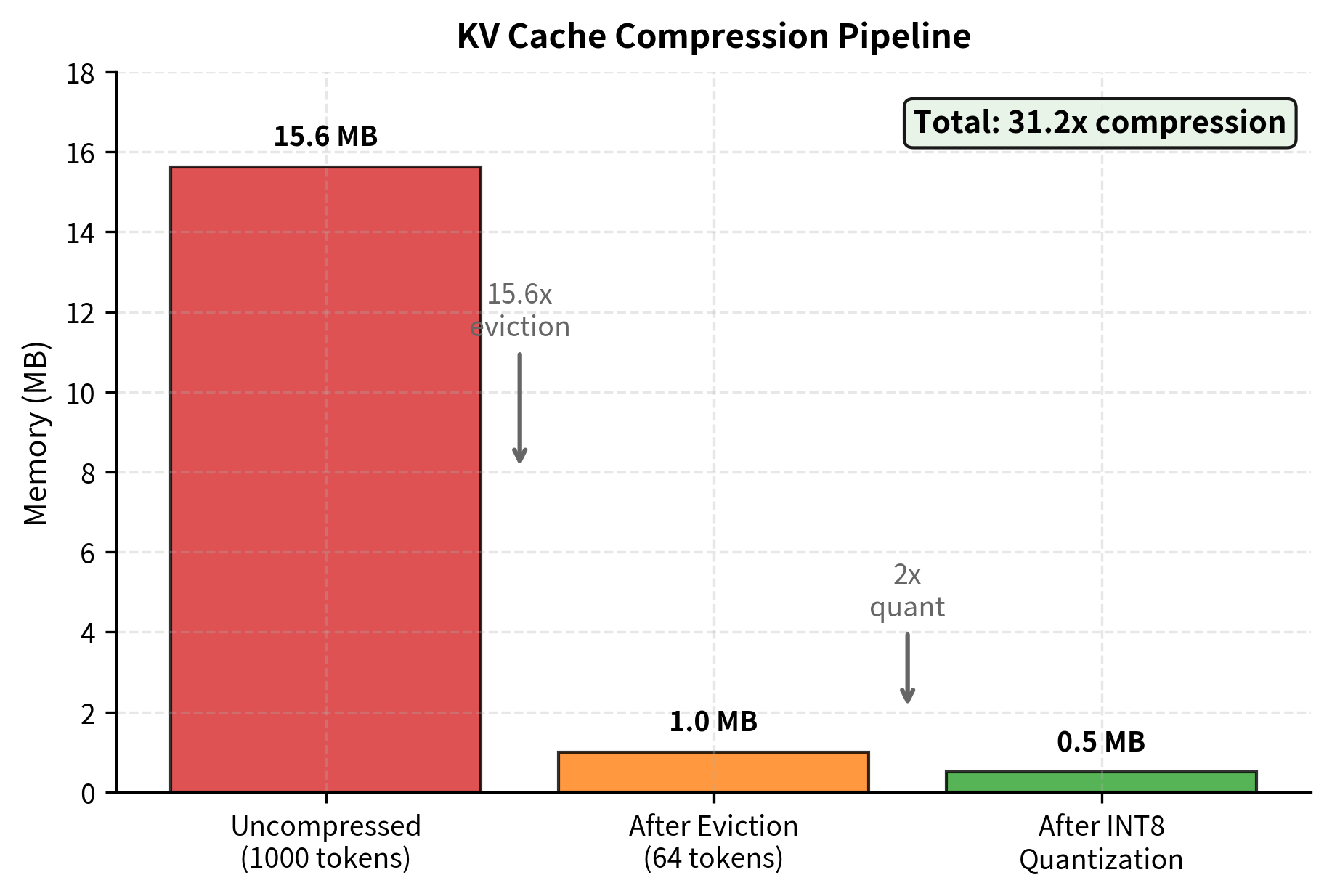
This level of compression enables generation at context lengths that would otherwise exceed available memory. A configuration that might require 16GB of KV cache memory without compression can operate within 500MB using these combined techniques. For deployment scenarios where memory is constrained or costs must be minimized, such aggressive compression makes previously infeasible applications practical.

Compression Quality AnalysisLink Copied

Compression introduces approximation error that can degrade generation quality, and understanding the nature of this error is essential for making informed trade-offs. Different compression techniques produce qualitatively different error patterns, which affects how they impact the attention mechanism and ultimately the generated text.

Let's visualize how different compression strategies affect the attention computation:

In[30]:

Code

import numpy as np

# Simulate a realistic attention pattern
np.random.seed(42)
seq_len = 64
query_len = 1

# Create attention weights with structure:
# - High attention to initial tokens (sinks)
# - Local attention to recent tokens
# - Sparse attention to intermediate tokens
attention_logits = np.random.randn(query_len, seq_len) * 0.5

# Add attention sink
attention_logits[:, :4] += 2.0

# Add local attention
attention_logits[:, -8:] += 1.5

# Add some heavy hitter tokens
attention_logits[:, 15] += 1.8
attention_logits[:, 28] += 2.0


# Softmax to get attention weights
def softmax(x):
    exp_x = np.exp(x - x.max(axis=-1, keepdims=True))
    return exp_x / exp_x.sum(axis=-1, keepdims=True)


original_attention = softmax(attention_logits)[0]

# Simulate quantization error (small random noise)
quant_noise = np.random.randn(seq_len) * 0.01
quantized_attention = softmax(attention_logits + quant_noise.reshape(1, -1))[0]

# Simulate eviction: only keep sink (4) + heavy hitters (4) + recent (8)
keep_mask = np.zeros(seq_len, dtype=bool)
keep_mask[:4] = True  # Sink
keep_mask[-8:] = True  # Recent
keep_mask[15] = True  # Heavy hitter
keep_mask[28] = True  # Heavy hitter

evicted_attention = np.zeros(seq_len)
evicted_logits = attention_logits.copy()
evicted_logits[:, ~keep_mask] = -1e9  # Mask evicted tokens
evicted_attention_computed = softmax(evicted_logits)[0]
evicted_attention[keep_mask] = evicted_attention_computed[keep_mask]

import numpy as np

# Simulate a realistic attention pattern
np.random.seed(42)
seq_len = 64
query_len = 1

# Create attention weights with structure:
# - High attention to initial tokens (sinks)
# - Local attention to recent tokens
# - Sparse attention to intermediate tokens
attention_logits = np.random.randn(query_len, seq_len) * 0.5

# Add attention sink
attention_logits[:, :4] += 2.0

# Add local attention
attention_logits[:, -8:] += 1.5

# Add some heavy hitter tokens
attention_logits[:, 15] += 1.8
attention_logits[:, 28] += 2.0


# Softmax to get attention weights
def softmax(x):
    exp_x = np.exp(x - x.max(axis=-1, keepdims=True))
    return exp_x / exp_x.sum(axis=-1, keepdims=True)


original_attention = softmax(attention_logits)[0]

# Simulate quantization error (small random noise)
quant_noise = np.random.randn(seq_len) * 0.01
quantized_attention = softmax(attention_logits + quant_noise.reshape(1, -1))[0]

# Simulate eviction: only keep sink (4) + heavy hitters (4) + recent (8)
keep_mask = np.zeros(seq_len, dtype=bool)
keep_mask[:4] = True  # Sink
keep_mask[-8:] = True  # Recent
keep_mask[15] = True  # Heavy hitter
keep_mask[28] = True  # Heavy hitter

evicted_attention = np.zeros(seq_len)
evicted_logits = attention_logits.copy()
evicted_logits[:, ~keep_mask] = -1e9  # Mask evicted tokens
evicted_attention_computed = softmax(evicted_logits)[0]
evicted_attention[keep_mask] = evicted_attention_computed[keep_mask]

Out[31]:

Visualization

Three heatmaps comparing original attention weights to compressed versions, showing quantization and eviction effects. — Impact of KV cache compression strategies on attention weight accuracy. While quantization introduces small, distributed errors across all positions, eviction causes binary information loss at removed locations. These error profiles show how the model maintains focus on semantic anchors even under aggressive compression.

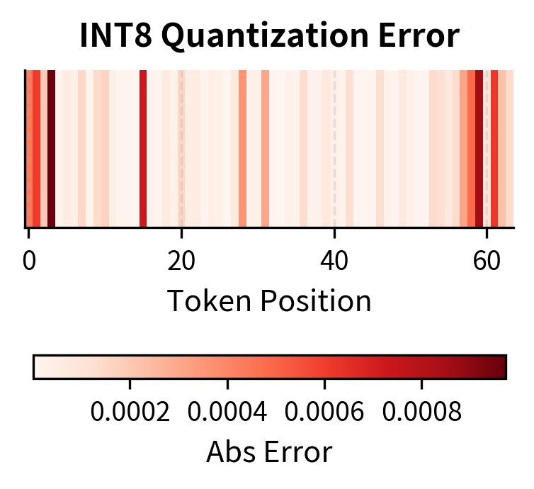
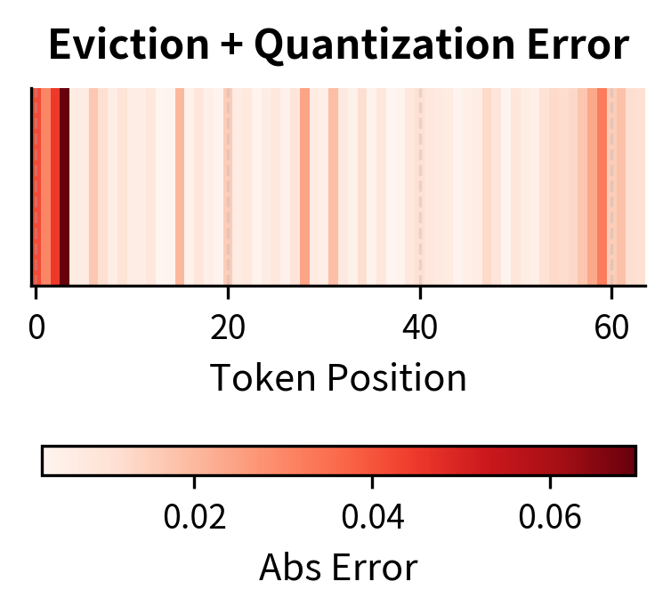
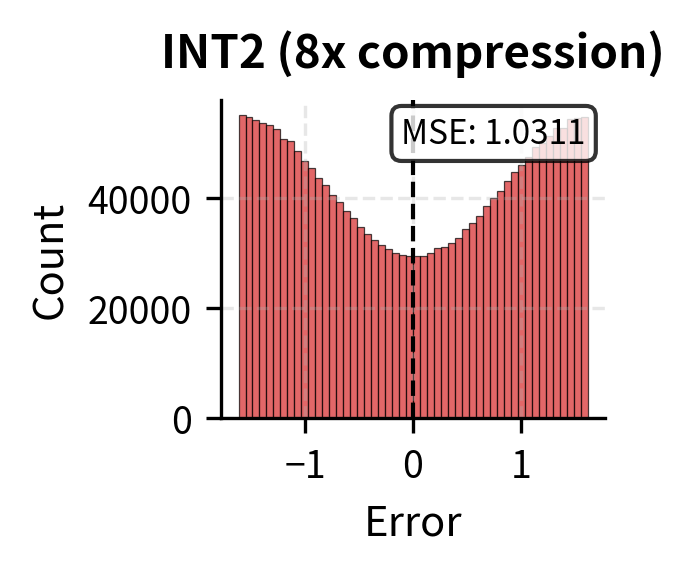
The visualization reveals the distinct error profiles of each compression technique, illustrating a fundamental difference in how they affect the attention computation. Quantization introduces small, distributed errors across all positions, preserving the overall attention pattern while adding noise uniformly. The relative importance of tokens remains intact, and the model can still attend to the information it needs, albeit with slight imprecision.

Eviction, by contrast, creates complete information loss for removed tokens. The error is not small and distributed but rather binary: retained tokens have zero error while evicted tokens have error equal to their original attention weight. The key to successful eviction is ensuring that evicted tokens would have received near-zero attention anyway. When this condition holds, the total attention error is minimal because we are only losing tokens that contributed negligibly. When eviction removes a token that the model would have attended to significantly, generation quality suffers because that information is permanently lost.

The H2O algorithm's tracking of cumulative attention helps identify which tokens can be safely removed by providing evidence of their historical importance. Tokens that have consistently received minimal attention are unlikely to suddenly become critical, making them safe eviction candidates. However, this heuristic is not perfect: a token that received little attention during the first 500 generation steps might become crucial at step 501 if the generated content shifts to reference that earlier context.

Limitations and Practical ConsiderationsLink Copied

KV cache compression involves fundamental trade-offs that you must understand. The most significant limitation is task sensitivity: some tasks are highly sensitive to long-range dependencies that may be evicted or distorted by compression. Summarization, question answering over long documents, and multi-hop reasoning can degrade significantly when important context is removed.

Eviction strategies face the challenge of predicting future importance from past attention. A token that received little attention during the first 500 generation steps might become crucial at step 501, but if it was evicted, that information is permanently lost. This is particularly problematic for tasks where relevance depends on the specific query or generated content. Heavy hitter detection helps, but cannot anticipate all future needs.

Quantization interacts with numerical precision in subtle ways. While INT8 typically works well, INT4 can cause issues for models that rely on precise attention scores. Grouped query attention and multi-query attention, as we covered in Part XIX, already reduce KV cache memory. Combining these architectural choices with aggressive quantization requires careful validation. The upcoming chapters on weight quantization will explore similar precision trade-offs in more depth.

Cache compression also complicates batched inference. Different sequences in a batch may have different important tokens, requiring either per-sequence eviction decisions (complex) or a union of important tokens across sequences (less aggressive compression). PagedAttention, covered in the previous chapter, handles this elegantly by allowing non-contiguous cache storage, but the combination with dynamic eviction adds implementation complexity.

Finally, the computational overhead of compression must be considered. Tracking cumulative attention scores, identifying heavy hitters, and performing quantization all consume compute and memory bandwidth. For latency-sensitive applications, the overhead may offset memory savings. Simple approaches like StreamingLLM's sink plus window strategy often provide the best latency-memory trade-off because they require no attention tracking.

Key ParametersLink Copied

The key parameters for KV cache compression are:

sink_size: Number of initial tokens to always preserve in the cache. These "attention sinks" are critical for stability.
window_size (or recent_size): Number of most recent tokens to keep. Ensures local context is available.
heavy_hitter_size: Number of high-attention tokens to preserve based on historical importance.
bits: Target bit width for quantization (e.g., 4 or 8). Lower bits save more memory but may increase error.

SummaryLink Copied

KV cache compression addresses the memory bottleneck of long-sequence generation through two complementary approaches: reducing the number of cached tokens through eviction, and reducing the precision of stored values through quantization.

Window-based eviction provides the simplest implementation but sacrifices all long-range context. Attention sink preservation recognizes that initial tokens serve as computational anchors and must be protected from eviction. The H2O algorithm extends this by tracking cumulative attention to identify and preserve "heavy hitter" tokens that consistently receive high attention, balancing recency with historical importance.

Cache quantization offers orthogonal memory savings. INT8 quantization typically achieves 2x compression with negligible quality impact. INT4 provides 4x compression but requires per-channel quantization and careful validation. Combining eviction with quantization can achieve compression ratios exceeding 30x for long sequences.

The choice of compression strategy depends on the specific use case. Tasks requiring precise long-range reasoning may tolerate only light compression, while streaming applications or tasks with primarily local dependencies can use aggressive compression. Understanding these trade-offs enables you to select appropriate configurations that balance memory efficiency with generation quality.

QuizLink Copied

Ready to test your understanding? Take this quick quiz to reinforce what you've learned about KV cache compression techniques.

Loading component...

Comments

Back to Language AI Handbook

Previous Chapter

Paged Attention

Next Chapter

Weight Quantization Basics

Reference

BIBTEXAcademic

@misc{kvcachecompressionevictionquantizationh2oalgorithm, author = {Michael Brenndoerfer}, title = {KV Cache Compression: Eviction, Quantization & H2O Algorithm}, year = {2026}, url = {https://mbrenndoerfer.com/writing/kv-cache-compression-eviction-quantization-h2o-algorithm}, organization = {mbrenndoerfer.com}, note = {Accessed: 2025-01-01} }

APAAcademic

Michael Brenndoerfer (2026). KV Cache Compression: Eviction, Quantization & H2O Algorithm. Retrieved from https://mbrenndoerfer.com/writing/kv-cache-compression-eviction-quantization-h2o-algorithm

MLAAcademic

Michael Brenndoerfer. "KV Cache Compression: Eviction, Quantization & H2O Algorithm." 2026. Web. today. <https://mbrenndoerfer.com/writing/kv-cache-compression-eviction-quantization-h2o-algorithm>.

CHICAGOAcademic

Michael Brenndoerfer. "KV Cache Compression: Eviction, Quantization & H2O Algorithm." Accessed today. https://mbrenndoerfer.com/writing/kv-cache-compression-eviction-quantization-h2o-algorithm.

HARVARDAcademic

Michael Brenndoerfer (2026) 'KV Cache Compression: Eviction, Quantization & H2O Algorithm'. Available at: https://mbrenndoerfer.com/writing/kv-cache-compression-eviction-quantization-h2o-algorithm (Accessed: today).

SimpleBasic

Michael Brenndoerfer (2026). KV Cache Compression: Eviction, Quantization & H2O Algorithm. https://mbrenndoerfer.com/writing/kv-cache-compression-eviction-quantization-h2o-algorithm

Direct link:

https://mbrenndoerfer.com/writing/kv-cache-compression-eviction-quantization-h2o-algorithm

About the author: Michael Brenndoerfer

All opinions expressed here are my own and do not reflect the views of my employer.

Michael currently works as an Associate Director of Data Science at EQT Partners in Singapore, leading AI and data initiatives across private capital investments.

With over a decade of experience spanning private equity, management consulting, and software engineering, he specializes in building and scaling analytics capabilities from the ground up. He has published research in leading AI conferences and holds expertise in machine learning, natural language processing, and value creation through data.

View Full Resume Publications Contact Books

KV Cache Compression: Eviction, Quantization & H2O Algorithm

KV Cache CompressionLink Copied

The Compression OpportunityLink Copied

Window-Based EvictionLink Copied

Attention-Based EvictionLink Copied

Attention Sink PreservationLink Copied

The H2O AlgorithmLink Copied

Cache QuantizationLink Copied

Per-Channel QuantizationLink Copied

Combining TechniquesLink Copied

Compression Quality AnalysisLink Copied

Limitations and Practical ConsiderationsLink Copied

Key ParametersLink Copied

SummaryLink Copied

QuizLink Copied

Comments

Reference

About the author: Michael Brenndoerfer

Related Content

GGUF Format: Efficient Storage & Inference for Quantized LLMs

AWQ: Protecting Salient Weights for Efficient LLM Inference

GPTQ: Optimizing 4-Bit Weight Quantization for LLMs

Stay updated

Comments

About the author: Michael Brenndoerfer

Related Content

GGUF Format: Efficient Storage & Inference for Quantized LLMs

AWQ: Protecting Salient Weights for Efficient LLM Inference

GPTQ: Optimizing 4-Bit Weight Quantization for LLMs

Stay updated