

Learn how PagedAttention uses virtual memory paging to eliminate KV cache fragmentation, enabling 5x better memory utilization in LLM serving systems.

This article is part of the free-to-read Language AI Handbook
Choose your expertise level to adjust how many terms are explained. Beginners see more tooltips, experts see fewer to maintain reading flow. Hover over underlined terms for instant definitions.
Paged Attention
In the previous two chapters, we explored how KV caches accelerate autoregressive generation by avoiding redundant computation, and we examined the substantial memory costs this optimization incurs. As we saw, a single 70B parameter model can require over 2.5 GB of KV cache memory per sequence at full context length. When serving multiple concurrent requests, this memory demand becomes the primary bottleneck limiting throughput.
But the raw memory consumption is only part of the story. Traditional KV cache implementations also face memory fragmentation. Even when the GPU has sufficient total free memory, the way that memory is allocated and deallocated can leave it unusable. This fragmentation can waste 60-80% of available KV cache memory, dramatically reducing the number of sequences a server can process simultaneously.
PagedAttention, introduced by the vLLM project in 2023, solves this fragmentation problem by borrowing a fundamental concept from operating systems: virtual memory with paging. Instead of allocating contiguous memory blocks for each sequence's KV cache, PagedAttention breaks the cache into fixed-size pages that can be stored anywhere in memory. This simple but powerful idea enables near-optimal memory utilization and has become the foundation for most modern LLM serving systems.
The Memory Fragmentation Problem
To understand why fragmentation occurs, we need to examine how traditional KV cache systems allocate memory. When a new request arrives, the system must reserve memory for the KV cache that will grow as tokens are generated. But here's the challenge: the system doesn't know in advance how long the final sequence will be.
The Contiguous Allocation Dilemma
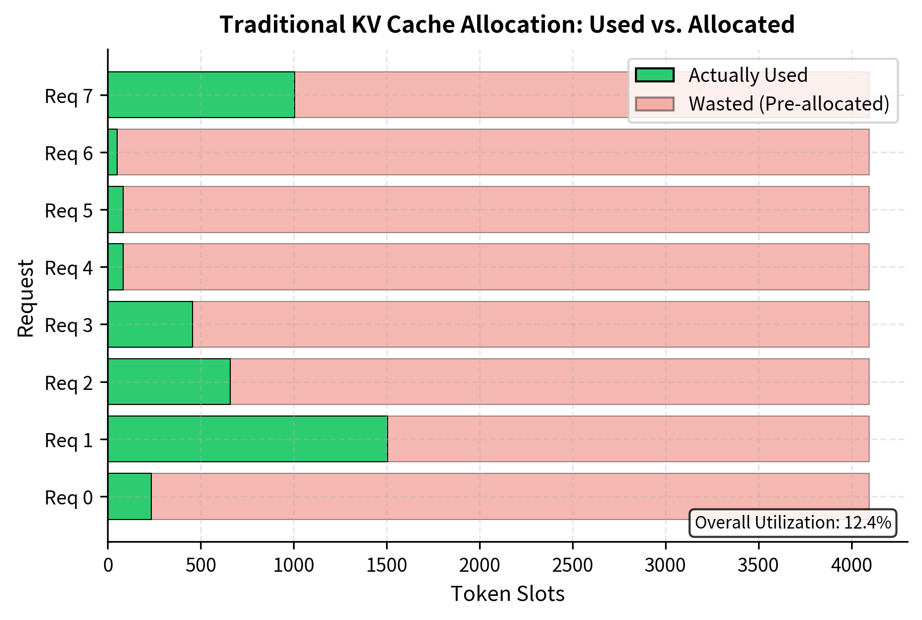
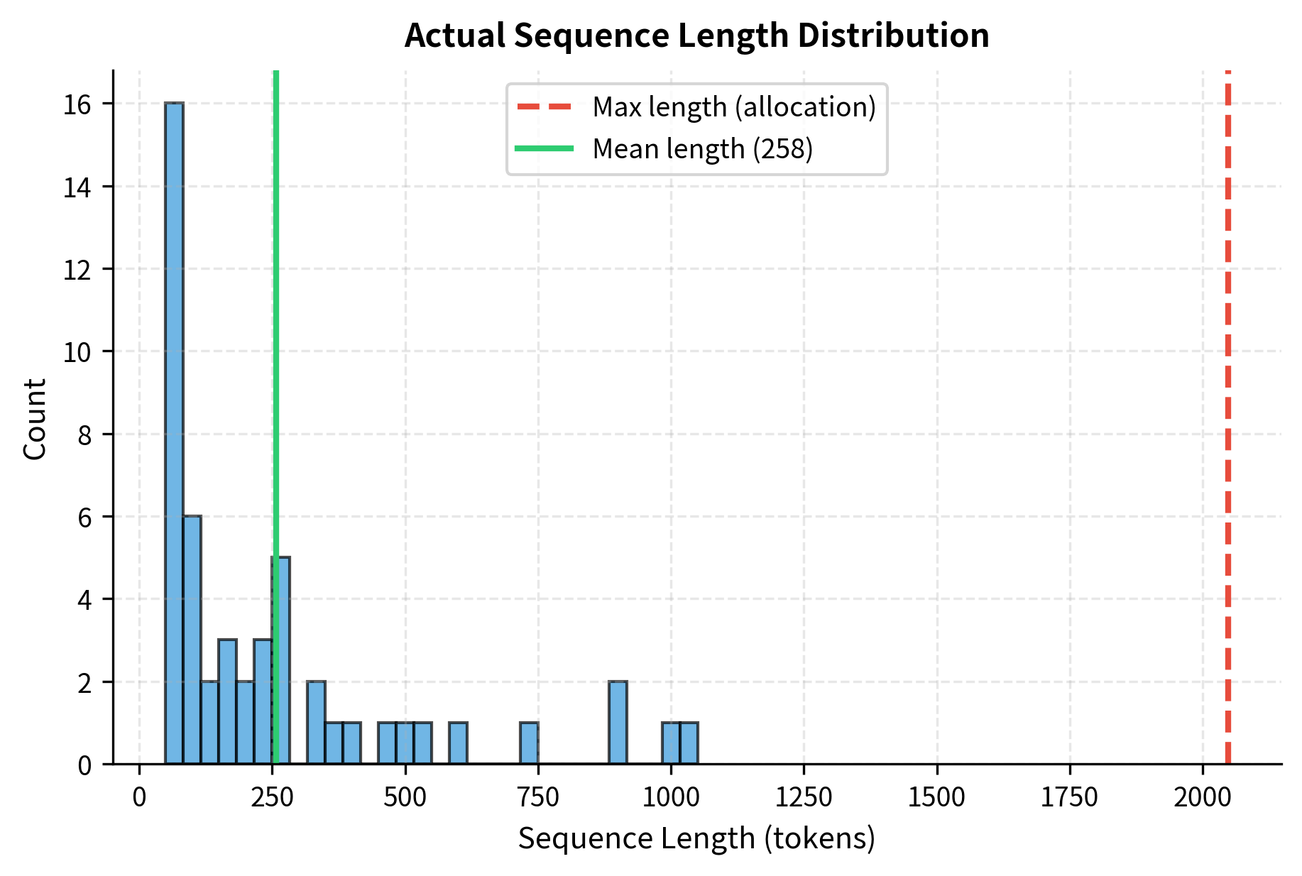
Traditional systems handle this uncertainty by pre-allocating memory based on the maximum possible sequence length. If your model supports 4,096 tokens, the system reserves space for all 4,096 KV pairs for each sequence, even if most requests only generate a few hundred tokens.
With realistic sequence length distributions, traditional allocation achieves only around 15% memory utilization. This means 85% of the reserved GPU memory sits unused, unable to serve additional requests.
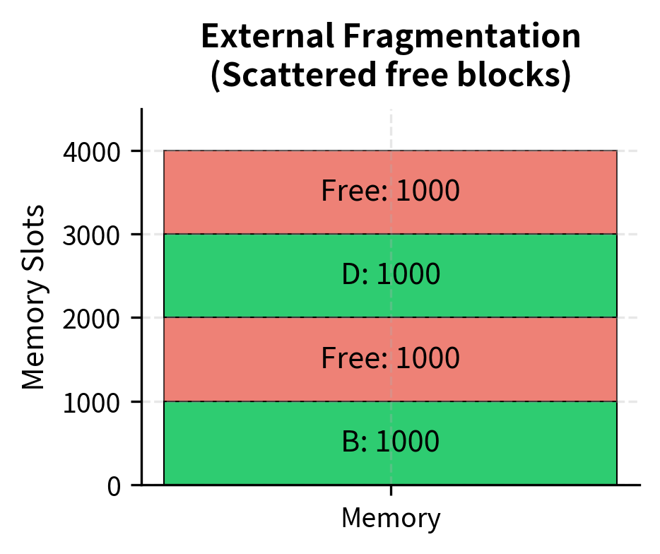
External Fragmentation
Even more problematic is external fragmentation, which occurs when requests complete and free their memory. Consider this scenario:
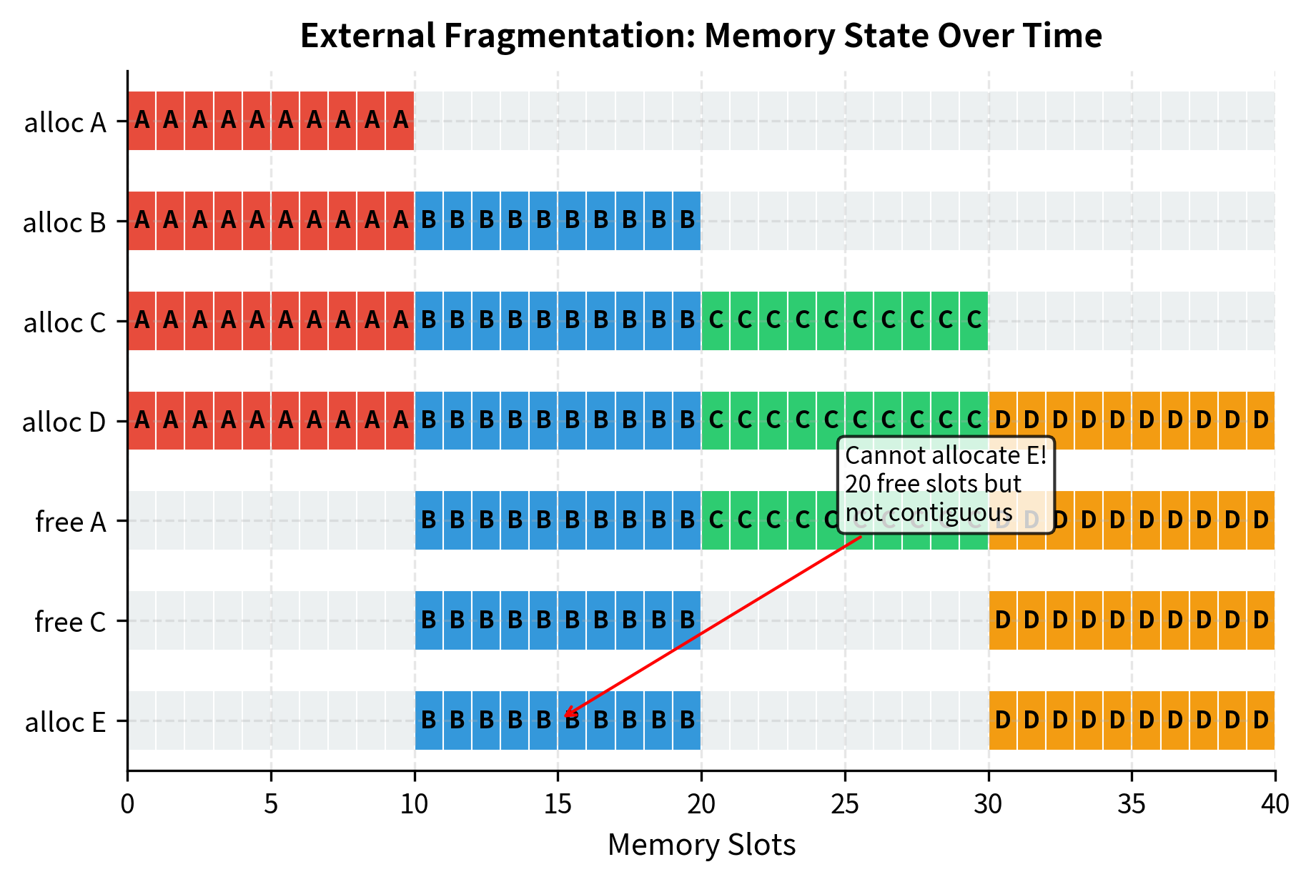
This is external fragmentation: the memory has 20 free slots, but they're split into two non-contiguous regions of 10 slots each. A new request requiring 10 contiguous slots cannot be served, even though sufficient total memory exists. In practice, with many concurrent requests starting and completing at different times, this fragmentation can become severe.
Internal Fragmentation
Internal fragmentation compounds the problem. When we allocate based on maximum sequence length but the actual sequence is shorter, the unused portion within the allocation is wasted:
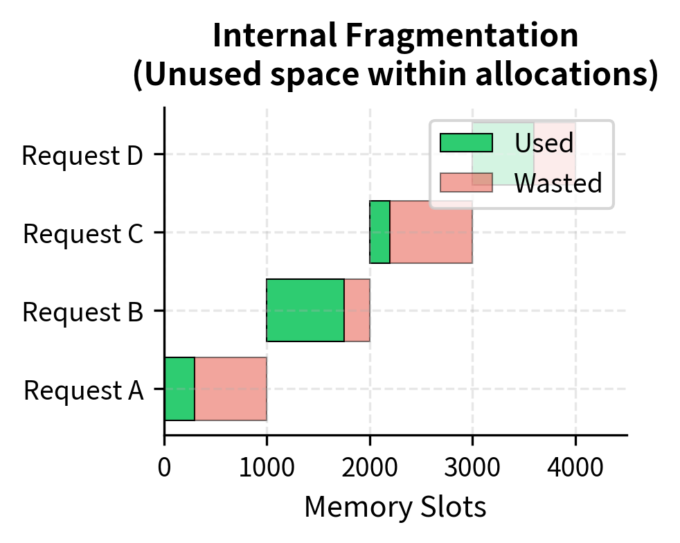
The combination of internal and external fragmentation means traditional serving systems achieve only 20-40% memory efficiency. For a GPU with 40 GB of KV cache capacity, this translates to effectively having only 8-16 GB available for actual use.
Page-Based Memory Allocation
The solution comes from a technique that operating systems have used for decades: virtual memory with paging. Instead of requiring contiguous physical memory, paging allows data to be stored in fixed-size blocks (pages) scattered anywhere in memory, with a page table tracking where each piece actually resides. This technique fundamentally changed operating system design in the 1960s, and it proves equally effective for managing KV caches in modern LLM serving systems.
The Paging Abstraction
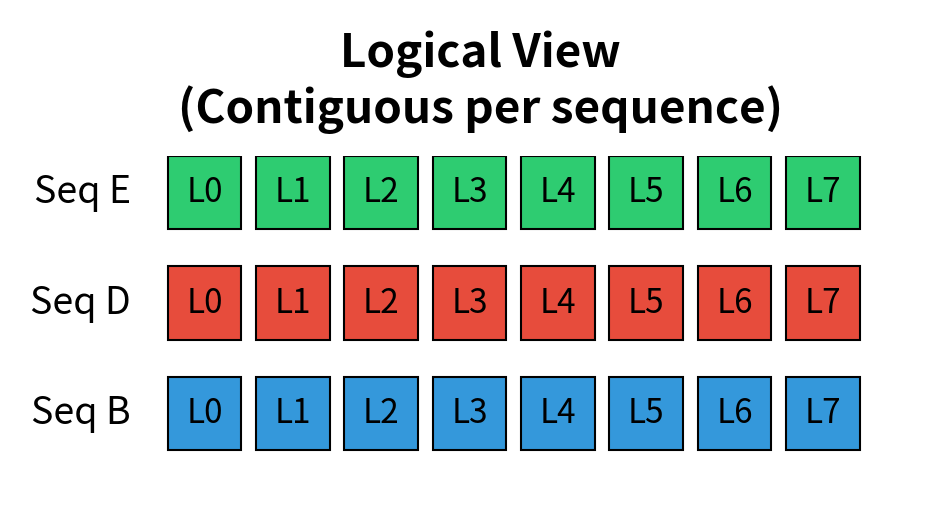
To understand how paging solves fragmentation, we must distinguish between logical and physical memory organization. A sequence's KV cache appears contiguous from a logical perspective, with tokens numbered 0, 1, 2, and so on. However, the actual physical storage need not mirror this logical arrangement. As long as we maintain a mapping that tells us where each piece of data resides in physical memory, we can store the data anywhere we like.
In the context of KV caches, paging works through four key concepts:
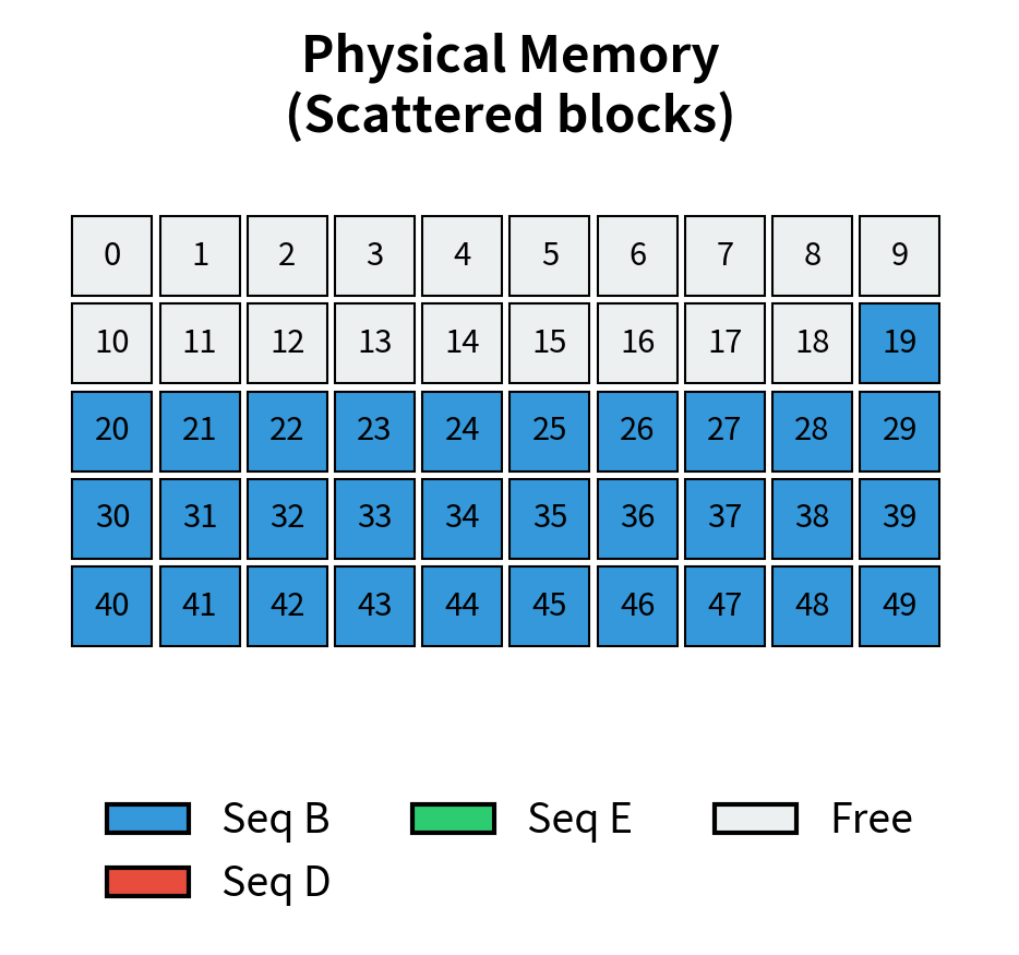
- Physical blocks: GPU memory is divided into fixed-size blocks, each capable of holding a small number of KV pairs (typically 16 tokens worth). These blocks represent the actual memory locations where data is stored.
- Logical blocks: Each sequence's KV cache is divided into logical blocks of the same size. These represent the abstract, contiguous view of the sequence's cache.
- Block table: A mapping from logical block indices to physical block locations. This data structure is the key that enables the translation between the sequence's logical view and the scattered physical reality.
- Dynamic allocation: Physical blocks are allocated only when needed, not pre-allocated. This on-demand approach means we never reserve memory for tokens that haven't been generated yet.
This approach decouples how we think about the data (logically contiguous per sequence) from how we store it (potentially scattered across physical memory). Let's implement a simulator to see these concepts in action:
No fragmentation! Request E was allocated using freed blocks from requests A and C, even though they're non-contiguous.
The key insight is that request E's blocks don't need to be contiguous in physical memory. The block table maintains the logical ordering, while physical blocks can be scattered anywhere. This eliminates external fragmentation entirely. When the simulator freed sequences A and C, their physical blocks returned to the free pool. Request E then claimed blocks from this pool, assembling its logical sequence from whatever physical locations happened to be available. From request E's perspective, it has a perfectly contiguous cache; the block table handles all the translation behind the scenes.
Block Table Structure
The block table is the critical data structure that enables this flexibility. For each sequence, it maintains an ordered list of physical block indices. The position in this list corresponds to the logical block number, while the value at that position indicates where in physical memory that block actually resides.
To visualize this concept, consider a sequence whose KV cache spans three logical blocks. The block table might contain the entries [7, 2, 15], indicating that logical block 0 is stored in physical block 7, logical block 1 is stored in physical block 2, and logical block 2 is stored in physical block 15. When the attention mechanism needs to access the key for token 20 (which falls in logical block 1, since each block holds 16 tokens), it consults the block table, finds that logical block 1 maps to physical block 2, and reads the data from that location.
Notice how sequence 4 (request E) uses physical blocks that are scattered throughout memory, reusing the blocks freed by sequences 0 and 2. From the sequence's perspective, it has a contiguous logical address space. The block table handles the translation.
This indirection through the block table introduces a small amount of overhead: every memory access must first look up the physical location. However, this cost is negligible compared to the enormous benefits of eliminating fragmentation. The block table itself is small, typically fitting entirely in fast GPU memory or cache, making lookups extremely fast.
The PagedAttention Algorithm
With KV cache data potentially scattered across non-contiguous memory locations, we need to modify the attention computation. The PagedAttention algorithm handles this by fetching keys and values according to the block table during attention calculation. This modification preserves the mathematical correctness of attention while accommodating the new memory layout.
Standard Attention vs PagedAttention
In standard attention, keys and values are stored in contiguous tensors. For a sequence of length , the attention mechanism computes a weighted sum of values based on the similarity between the query and keys:
where:
- : the query matrix (typically for the current token being generated)
- : the key matrix containing keys for all tokens in the sequence (contiguous tensor of shape )
- : the value matrix containing values for all tokens in the sequence (contiguous tensor of shape )
- : the dimension of the key vectors
- : the dimension of the value vectors
- : the sequence length
- : the function that normalizes similarity scores into probabilities
The formula consists of three computational stages. First, the dot product measures the similarity between the query and each key. Intuitively, this operation asks "how relevant is each previous token to the token we're currently generating?" Keys that are more similar to the query receive higher scores, indicating greater relevance. The result is a vector of raw similarity scores, one for each position in the sequence.
The second stage applies the function to these raw scores. This normalization transforms the arbitrary similarity values into a proper probability distribution that sums to 1. The softmax operation has an important property: it accentuates differences, making high scores relatively higher and low scores relatively lower. The output is the attention weights, which tell us how much to attend to each previous position.
The third stage multiplies these attention weights by the value matrix , computing a weighted average of the value vectors. Tokens with higher attention weights contribute more to the final output, while tokens with lower weights contribute less. This mechanism allows the model to selectively focus on the most relevant information from the context.
The division by in the formula ensures numerical stability. Without this scaling factor, the dot products between queries and keys tend to grow large as the dimension increases. Large dot products cause the softmax function to saturate, producing attention distributions that are nearly one-hot (all attention on one token). The scaling factor keeps the dot products in a reasonable range, allowing the softmax to produce more nuanced attention patterns and improving numerical stability during training and inference.
In PagedAttention, and are stored in non-contiguous blocks rather than contiguous tensors. The attention computation must gather the relevant blocks according to the block table. While the mathematical operation remains identical, the implementation must navigate the scattered physical layout:
This reference implementation shows the core idea: before computing attention, we gather the keys and values from their physical locations according to the block table. The attention computation itself remains unchanged. The gathering process iterates through logical block indices, looks up the corresponding physical block in the block table, and fetches the data from that physical location. Once all the keys and values are assembled into contiguous tensors, the standard attention formula applies.
Demonstration with Non-Contiguous Blocks
Let's verify that PagedAttention produces correct results even when blocks are scattered:
Optimized CUDA Kernels
The reference implementation above gathers blocks into contiguous memory before computing attention. This defeats some of the purpose of paging, as it requires temporary memory allocation. Production implementations like vLLM use custom CUDA kernels that compute attention directly on the paged data structure, avoiding the explicit gather step entirely.
The key optimization insight is that attention can be computed incrementally as blocks are loaded, rather than requiring all data to be assembled first. This approach leverages the online softmax algorithm (also known as the flash attention technique from Part XIV, Chapter 8) to maintain numerical stability while processing blocks one at a time. The online softmax technique keeps a running maximum and a running sum, updating them as each new block is processed. This allows the kernel to compute the final attention output without ever needing to store all the keys and values in a contiguous buffer.
The critical optimization is computing attention incrementally as blocks are loaded, rather than gathering all blocks first. This approach uses the online softmax algorithm (also known as the flash attention technique from Part XIV, Chapter 8) to maintain numerical stability while processing blocks one at a time. By processing blocks sequentially and maintaining running statistics, the kernel achieves the same mathematical result as gathering all keys first, but with dramatically reduced memory requirements.
vLLM Implementation
vLLM (Variational Large Language Model serving) is the framework that introduced PagedAttention. Understanding its architecture reveals how paging integrates into a complete serving system.
Memory Manager
The vLLM BlockSpaceManager handles physical block allocation:
Freed blocks from sequence 1 are available for reuse!
The simulation illustrates the manager's efficiency: when Sequence 1 completes, its blocks are immediately returned to the free pool. These reclaimed blocks are then available for Sequence 0's expansion or new requests, preventing the memory fragmentation issues seen in static allocation.
Copy-on-Write for Beam Search
One elegant feature of paged memory is enabling copy-on-write (CoW) semantics for parallel decoding strategies like beam search. This technique addresses a fundamental challenge in beam search: multiple candidate sequences (beams) that share a common prefix would traditionally require duplicating the KV cache data for that prefix, even though it's identical across all beams.
With copy-on-write, when multiple beams share a common prefix, they can share the same physical blocks for that prefix rather than duplicating the data. The block manager tracks reference counts for each physical block. When a block has multiple references, it means multiple sequences are sharing that block. Only when a sequence needs to modify a shared block does the system create a copy, hence the name "copy-on-write."
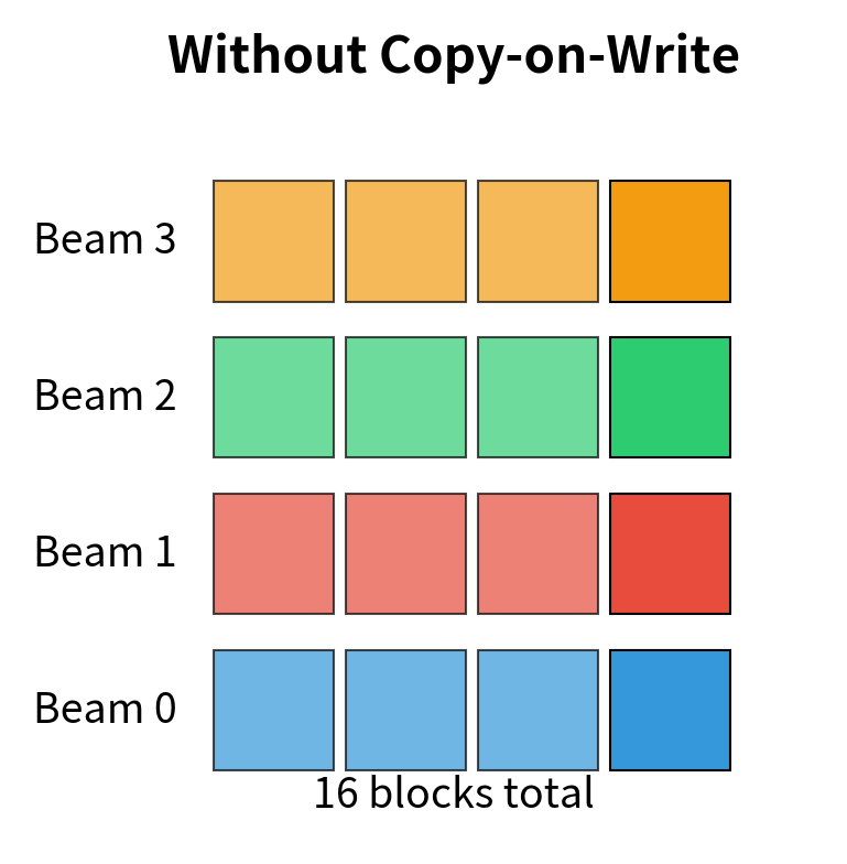
To understand why this matters, consider a beam search with width 4. Without copy-on-write, each beam would need its own complete copy of the KV cache, requiring 4x the memory. With copy-on-write, all four beams share the physical blocks for their common prefix. Memory is only allocated separately when the beams diverge and generate different tokens.
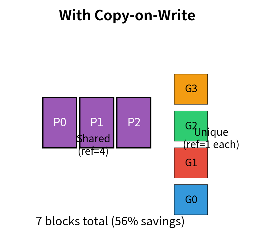
This 25% memory reduction highlights the efficiency of copy-on-write. By allowing multiple beams to share the same physical blocks for their common prefix, we significantly reduce memory footprint compared to duplicating the data for each beam. The savings become even more dramatic with longer prompts or wider beam widths, as the shared prefix represents a larger fraction of the total cache.
Working with vLLM in Practice
Let's see how PagedAttention benefits manifest when using vLLM for inference:
Key Parameters
The key parameters for vLLM related to PagedAttention are:
- block_size: Number of tokens per physical block. Smaller blocks reduce internal fragmentation but increase block table overhead.
- gpu_memory_utilization: Fraction of GPU memory reserved for KV cache. Higher values enable more concurrent sequences.
- max_num_seqs: Maximum concurrent sequences. PagedAttention enables much higher limits than traditional approaches.
- swap_space: CPU memory for block swapping when GPU memory is exhausted.
Measuring Fragmentation Reduction
Let's quantify the improvement PagedAttention provides over traditional allocation:
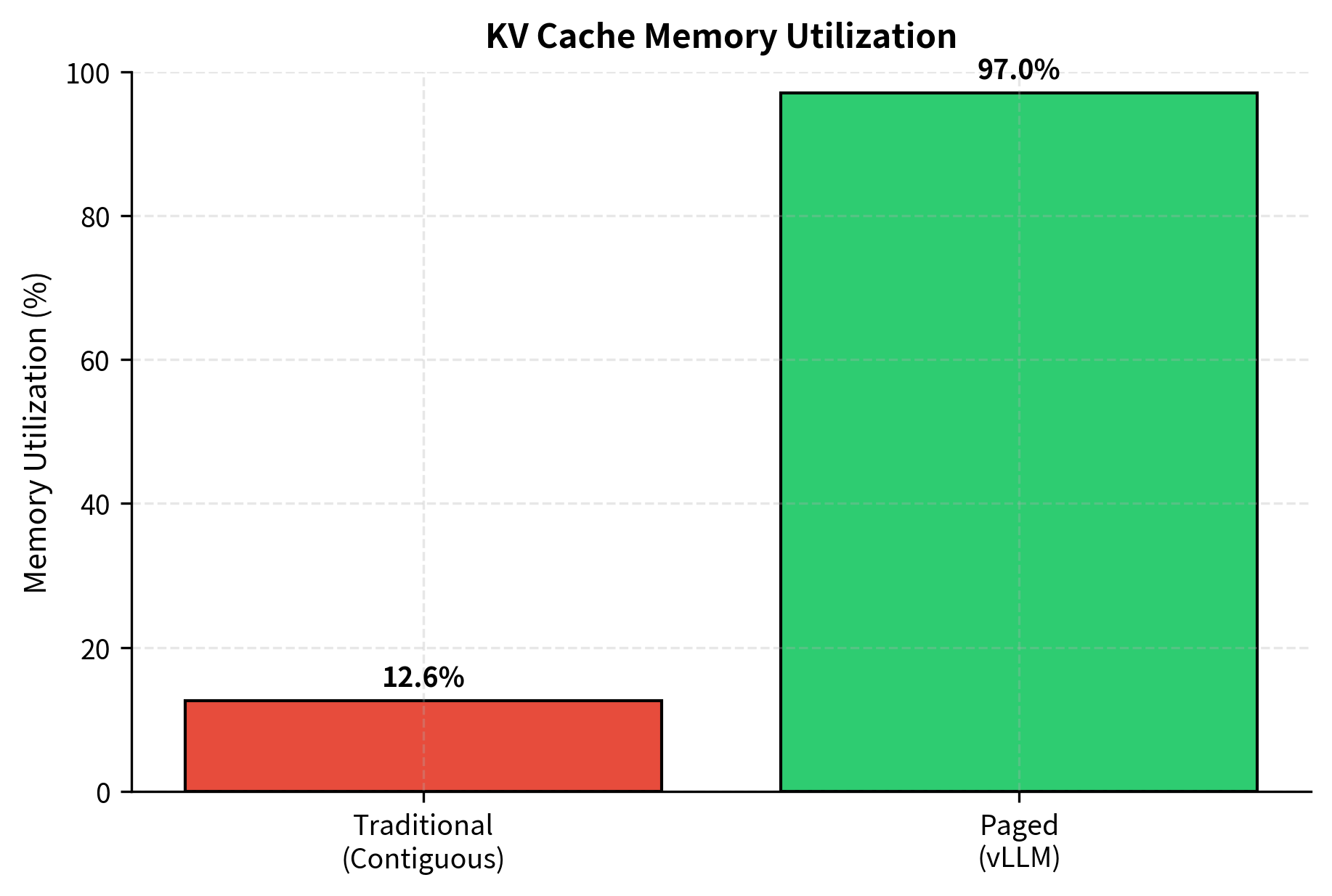
These results highlight the massive inefficiency of contiguous allocation. By switching to paged allocation, we effectively reclaim 80% of the memory that was previously wasted on fragmentation, allowing us to serve five times as many sequences with the same hardware.
Benefits and Performance Impact
PagedAttention provides several interconnected benefits that compound to deliver substantial throughput improvements.
Higher Batch Sizes
The most direct benefit is the ability to serve more concurrent sequences. With 5x better memory utilization, a serving system can batch 5x more requests simultaneously. Since transformer inference is typically compute-bound for large batches, higher batch sizes improve GPU utilization:
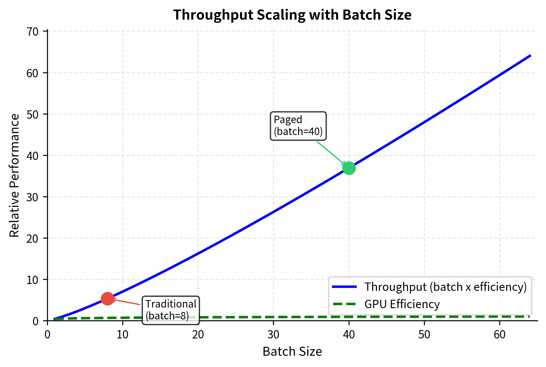
The throughput improvement demonstrates that memory efficiency directly translates to performance. By fitting more sequences into the GPU, we operate in a regime of higher compute intensity, extracting more value from the hardware.
Dynamic Batching Support
Paged memory enables continuous batching (which we'll explore in an upcoming chapter), where new requests can join an ongoing batch as old ones complete. With traditional contiguous allocation, adding a new request requires finding a large enough contiguous memory region. With paging, new requests simply acquire free blocks as needed:
Paged allocation significantly outperforms the traditional approach in dynamic settings. While the traditional allocator quickly becomes fragmented and unable to accept new requests, the paged allocator continuously reuses freed blocks, maintaining high throughput and minimizing queue times.
Preemption and Priority Scheduling
With paged memory, preempting a low-priority request to serve a high-priority one becomes straightforward. The preempted request's blocks can be either swapped to CPU memory or simply marked as reusable. When the request resumes, it reloads from the saved state. This enables sophisticated scheduling policies that traditional contiguous allocation cannot support.
Limitations and Practical Considerations
While PagedAttention represents a major advancement in LLM serving efficiency, it comes with trade-offs and limitations worth understanding.
The most significant overhead is the block table indirection. Every attention computation must look up physical block locations from the block table, adding memory access latency. For very short sequences, this overhead can outweigh the benefits of paging. In practice, the crossover point occurs around 50-100 tokens; shorter sequences may actually perform better with contiguous allocation. Most serving workloads involve longer sequences where the memory efficiency gains far exceed the indexing overhead.
Block size selection presents a tuning challenge. Smaller blocks reduce internal fragmentation (waste from partially-filled blocks) but increase the block table size and lookup overhead. Larger blocks are more efficient for the attention computation but waste more memory on partial fills. The default block size of 16 tokens in vLLM represents a carefully chosen balance, but optimal values vary with workload characteristics. Workloads with highly variable sequence lengths benefit from smaller blocks, while uniform-length workloads can use larger blocks.
Implementing PagedAttention is complex. Custom CUDA kernels must handle the non-contiguous memory access patterns efficiently, maintaining the performance characteristics of optimized attention implementations like FlashAttention while adding paging support. This is why you should use established frameworks like vLLM rather than implementing PagedAttention from scratch.
Finally, PagedAttention addresses memory capacity constraints but not the fundamental memory bandwidth limitations discussed in earlier chapters. The KV cache still requires significant memory bandwidth to read during attention computation. Techniques we'll explore in upcoming chapters, such as KV cache compression and quantization, complement PagedAttention by reducing the size of the data that must be transferred.
Summary
PagedAttention transforms LLM inference efficiency by applying virtual memory principles to KV cache management. The key insights and techniques include:
-
The fragmentation problem arises because traditional KV cache allocation reserves contiguous memory based on maximum sequence length. This causes internal fragmentation (unused space within allocations) and external fragmentation (scattered free blocks that cannot be combined). Together, these issues can waste 60-80% of available memory.
-
Page-based allocation divides memory into fixed-size blocks that can be assigned to any sequence. A block table maps each sequence's logical blocks to their physical locations. This approach eliminates external fragmentation entirely and reduces internal fragmentation to at most one partial block per sequence.
-
The PagedAttention algorithm modifies attention computation to work with non-contiguous KV storage. During attention, keys and values are gathered according to the block table. Optimized CUDA kernels perform this gathering efficiently using online softmax techniques to avoid explicit memory reordering.
-
Copy-on-write semantics enable memory-efficient beam search and other parallel decoding strategies. Sequences can share physical blocks for common prefixes, with new blocks allocated only when sequences diverge.
-
Practical benefits include 2-4x higher throughput from increased batch sizes, support for continuous batching with dynamic request handling, and preemption capabilities for priority scheduling. These improvements have made PagedAttention the foundation of modern LLM serving systems like vLLM, TensorRT-LLM, and others.
Quiz
Ready to test your understanding? Take this quick quiz to reinforce what you've learned about PagedAttention and memory management for LLM serving.

Comments