KV Cache Memory: Calculating GPU Requirements for LLM Inference

In the previous chapter, we saw how the KV cache eliminates redundant computation during autoregressive generation by storing keys and values from previous tokens. This memory-compute tradeoff is fundamental to efficient inference. However, as models grow larger and context windows expand, the KV cache can consume enormous amounts of GPU memory.

Understanding exactly how much memory the KV cache requires is essential for deployment planning. A seemingly A seemingly simple question: "Can I run this model on my GPU?" requires knowing not just the model weight size but also how much memory the cache will consume during generation. The answer depends on the model architecture, the sequence length, the batch size, and the data type. This chapter provides the tools to calculate these requirements precisely.

Before calculating memory requirements, we need to understand exactly what the cache stores. Recall from the previous chapter that during each forward pass, we cache the key and value projections for reuse in subsequent tokens. This caching strategy transforms what would be repeated linear projections into simple memory lookups. However, every lookup requires that the data exist in GPU memory. Understanding the precise shape and structure of this stored data is the first step toward calculating its memory footprint.

The keys and values we cache are not arbitrary tensors. They have very specific shapes determined by the attention mechanism's design. When attention processes a token, it creates a query vector to ask "what should I attend to?" Corresponding key and value vectors for that token answer questions from future tokens. The query is used immediately and discarded, but the keys and values must persist because future tokens will compare against them.

For a single attention layer processing a single token, the projections produce:

• Key tensor: shape [batch_size, num_kv_heads, 1, head_dim]
• Value tensor: shape [batch_size, num_kv_heads, 1, head_dim]

The "1" in these shapes represents the single token being processed during generation. This single-token slice is what gets appended to the existing cache with each forward pass. The batch dimension allows processing multiple independent sequences simultaneously, the head dimension captures the multi-head structure of attention, and the head_dim represents the dimensionality of each head's representation space.

After processing $t$ tokens, the accumulated cache for that layer has:

• Key cache: shape [batch_size, num_kv_heads, t, head_dim]
• Value cache: shape [batch_size, num_kv_heads, t, head_dim]

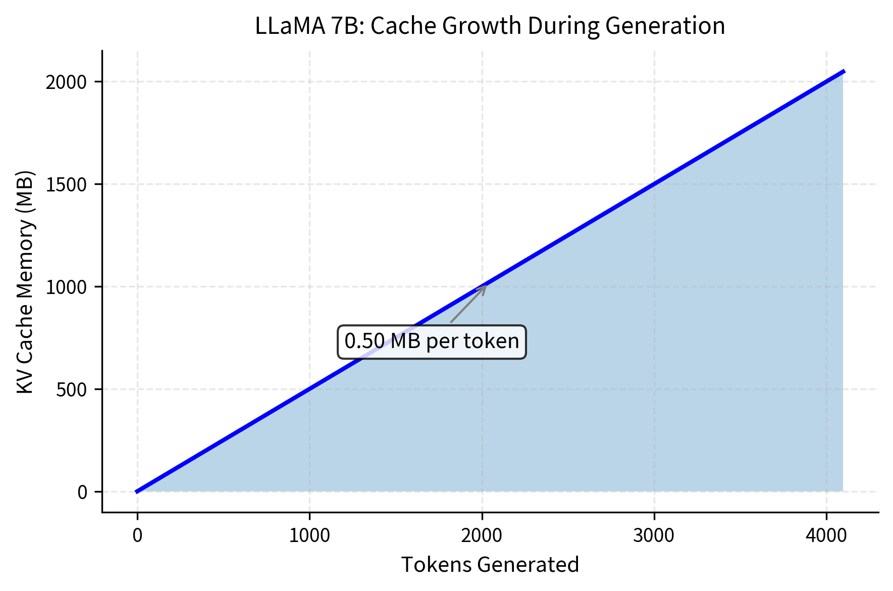
Notice how the sequence dimension grows from 1 to $t$ as tokens accumulate. This growth is the source of the linear memory scaling that dominates long-context inference. Each new token adds one slice along the sequence dimension, which must be stored for all subsequent generation steps.

The full KV cache spans all transformer layers. A model with $L$ layers maintains $L$ key caches and $L$ value caches. This multiplicative effect of layers is crucial: a 32-layer model requires 32 times the cache of a single layer, making the number of layers one of the primary drivers of total cache size. Each layer's cache is completely independent, containing that layer's unique representation of the sequence history.

The data type determines bytes per element. Most modern inference uses half-precision (FP16 or BF16) at 2 bytes per element, though some systems use FP32 (4 bytes) or quantized representations like INT8 (1 byte) or INT4 (0.5 bytes). This choice creates a direct tradeoff between precision and memory consumption. Halving the bytes per element halves the cache size, which is why quantization techniques have become essential for deploying large models.

With a clear understanding of what the cache stores, we can now derive the formula for total memory consumption. The calculation follows directly from multiplying the dimensions of the cached tensors by the number of bytes each element requires. This derivation provides the foundation for all deployment planning decisions.

Consider the structure we described above. For each layer, we store both keys and values. Each of these has shape [batch_size, num_kv_heads, seq_len, head_dim]. The total number of elements in one such tensor is the product of these dimensions. Since we store two tensors (keys and values) per layer across all layers, the total element count becomes:

Converting elements to bytes requires multiplying by the bytes per element, giving us the complete formula:

where:

• $2$ accounts for storing both key and value matrices
• $L$: the number of transformer layers
• $B$: the batch size
• $T$: the sequence length (number of tokens cached)
• $H_{\text{kv}}$: the number of key-value heads
• $D_h$: the head dimension
• $\text{bytes}$: the number of bytes per element (2 for FP16, 4 for FP32)

This formula reveals the linear dependencies that govern cache memory. Doubling any of the multiplicative factors doubles the total memory. This linearity is both a blessing and a curse. It makes calculations simple and predictable, but it also means there are no economies of scale. Processing twice as many tokens always requires twice as much cache memory, with no possibility of compression through clever algorithms (unless we explicitly introduce approximation techniques covered in later chapters).

For standard Multi-Head Attention (MHA), $H_{kv}$ equals the number of attention heads $H$, and $H \times D_h = D_{model}$. This relationship exists because each head operates on a slice of the model dimension, and together all heads span the full representation space. This architectural constraint allows us to simplify our formula:

where:

• $D_{\text{model}}$ is the model dimension (equal to $H \times D_h$, representing the total embedding size)
• $L$: the number of transformer layers
• $B$: the batch size
• $T$: the sequence length
• $\text{bytes}$: the number of bytes per element

This simplified form is particularly useful because $D_{model}$ is typically reported in model documentation, making quick mental calculations possible. For example, knowing that a model has dimension 4096, 32 layers, and you want to cache 4096 tokens in FP16, you can quickly compute: $2 \times 32 \times 1 \times 4096 \times 4096 \times 2$ bytes, which equals roughly 2 GB.

For models using Grouped Query Attention (GQA), which we covered in Part XIX, the number of KV heads is smaller than the number of query heads. This architectural innovation allows multiple query heads to share the same key-value pairs, dramatically reducing the cache footprint. GQA achieves this without proportionally harming model quality. If a model has $H$ query heads but only $H_{kv}$ key-value heads, the cache size reduces proportionally:

where:

• $H$ is the number of query attention heads
• $H_{\text{kv}}$ is the number of key-value heads

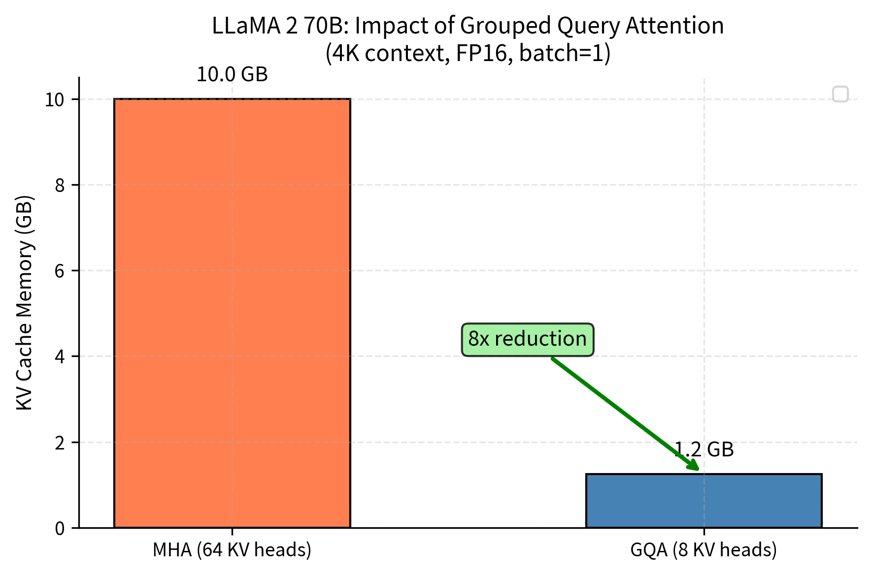
This reduction factor quantifies the memory savings from GQA. A model with 64 query heads and 8 KV heads achieves an 8× reduction in cache size compared to standard MHA. This 8× reduction makes large models feasible on single GPUs instead of requiring expensive multi-GPU clusters.

Now let's examine concrete examples with popular model architectures. First, we define our model specifications and a calculation function:

These results reveal several important patterns about KV cache scaling across different architectures. For GPT-2, the cache remains negligible relative to model weights, consuming only about 2-3% of total memory. However, as we scale to larger models like LLaMA 7B, the cache becomes more significant, reaching approximately 7-8% of weight memory at 4K context. The most striking pattern appears with LLaMA 2 and 3 70B models. Despite being 10× larger than LLaMA 7B, their use of Grouped Query Attention with only 8 KV heads means their cache is actually smaller than LLaMA 7B's cache, demonstrating an 8× reduction compared to what standard multi-head attention would require. This architectural choice makes the difference between practical deployment and memory constraints that would require multiple GPUs.

Several patterns emerge from this comparison. GPT-2's KV cache is negligible relative to its weights. But as models scale up, the cache becomes increasingly significant. For LLaMA 7B at 4096 tokens, the cache is already a measurable percentage of the model weight memory. The benefit of GQA becomes clear with LLaMA 2 70B: using 8 KV heads instead of 64 reduces cache size by 8×. This dramatic reduction makes large model deployment feasible within typical GPU memory constraints.

Sequence length has a linear effect on KV cache size. This relationship emerges directly from our formula. The term $T$ (sequence length) appears as a simple multiplicative factor, meaning that doubling the context window doubles the cache memory. Unlike attention score computation, which grows quadratically with sequence length, cache memory grows strictly linearly. This linear relationship enables straightforward capacity planning and creates unavoidable memory costs for long contexts.

This linear relationship becomes particularly problematic for long-context models. The trend in language model development has been toward ever-longer context windows, from 512 tokens in early BERT models to 128K or even 1M token windows in modern systems. Every tenfold increase in context length requires tenfold more cache memory, creating a fundamental tension between capability and resource requirements.

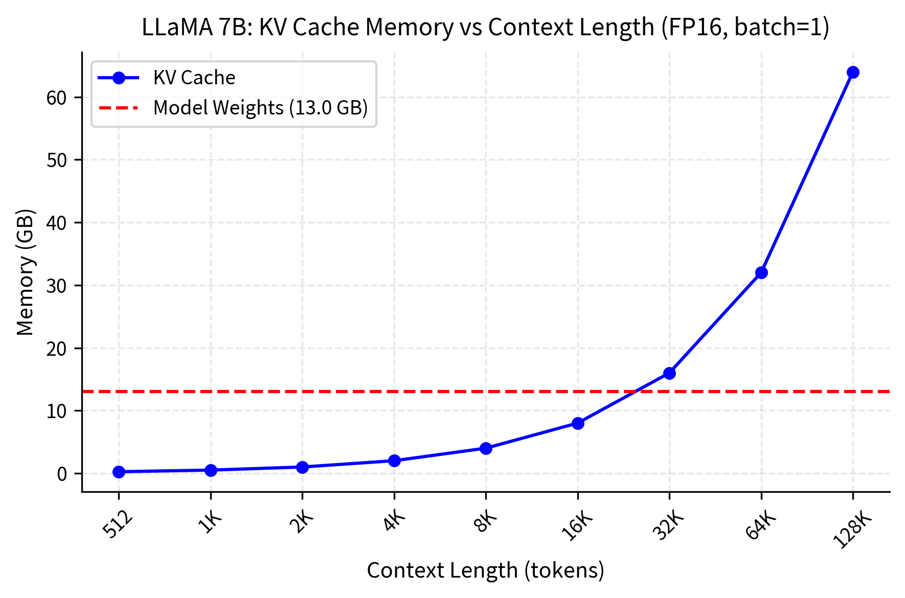
The crossover point, where KV cache exceeds model weights, is critical for deployment planning. This visualization clearly shows the linear relationship between sequence length and memory consumption, with the cache becoming the dominant memory consumer at longer contexts. Let's find it exactly:

This crossover point represents a fundamental shift in the memory profile of inference. Below this threshold, model weights dominate memory consumption and the cache is a relatively small overhead. Above this threshold, the cache becomes the primary memory consumer, growing linearly with every additional token while weights remain constant. For context windows beyond approximately 32K tokens, the KV cache will consume more memory than the model itself, fundamentally changing deployment requirements and making cache optimization techniques essential rather than optional.

At this crossover point, the KV cache memory equals the model weight memory. For context lengths beyond this point, the cache becomes the dominant memory consumer, fundamentally changing the memory profile of inference.

For long-context applications such as document analysis, multi-turn conversations, and code completion, the KV cache dominates memory usage. A 128K context window, as supported by models like Claude and GPT-4, would require 32× more cache memory than a 4K window. This scaling explains why long-context inference often requires specialized infrastructure and optimization techniques that would be unnecessary for short-context applications.

Batch size also scales linearly with cache memory, following the same multiplicative relationship we observed with sequence length. Each sequence in the batch maintains its own independent cache. Tokens in one sequence do not attend to tokens in another sequence, so cached values are not shared across batch elements. Each sequence maintains independent keys and values accessed only by its own future tokens.

This independence has important implications for memory planning. If you want to process 8 concurrent requests, you need 8 complete copies of the KV cache (one for each sequence). The batch dimension in our cache tensors, represented by $B$ in our formula, is not a clever abstraction that enables sharing; it simply organizes multiple independent caches for efficient parallel processing.

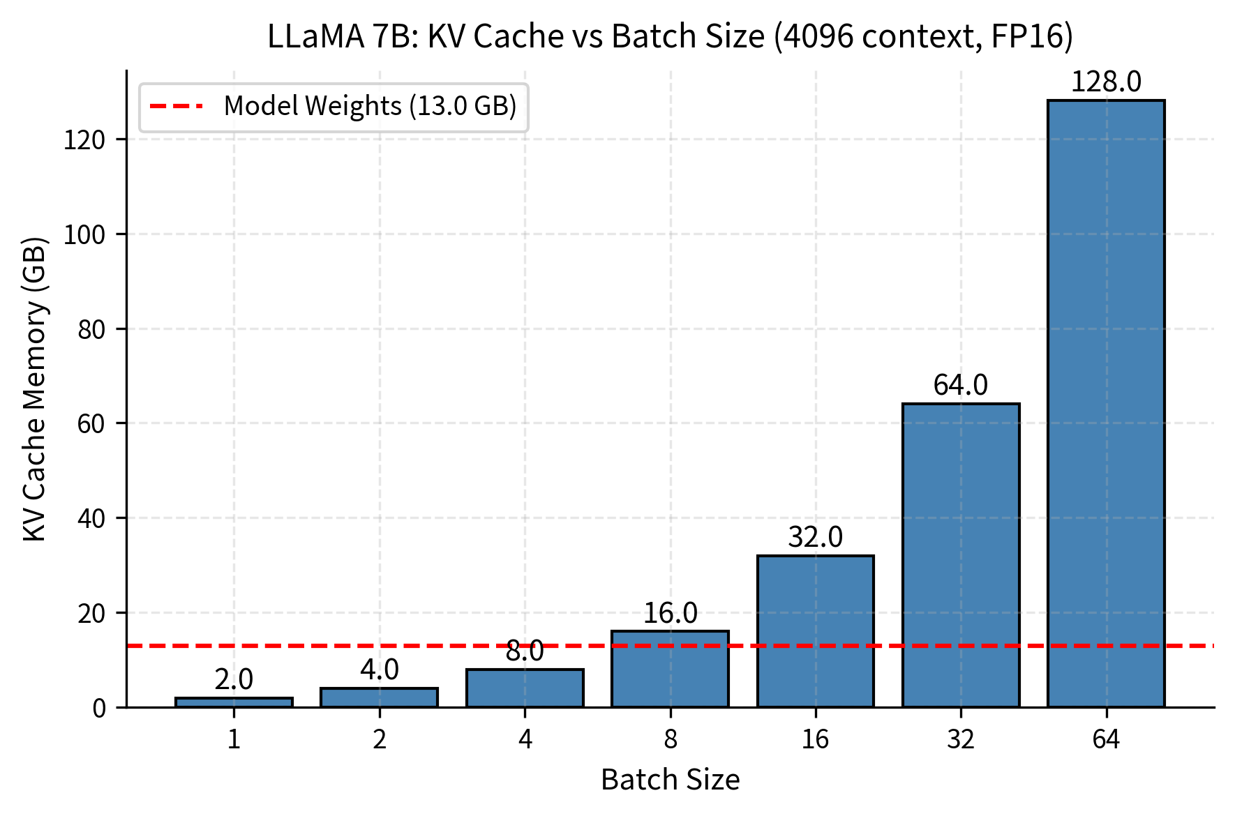
This visualization clearly demonstrates the linear relationship between batch size and KV cache memory. The batch size tradeoff is fundamental to inference economics, as it directly determines the throughput your system can achieve in production deployment. Doubling batch size doubles memory requirements, but it also doubles the number of requests you can process in parallel. This creates a direct tension between throughput and memory availability:

• Single-sequence inference minimizes cache memory but leaves GPU compute underutilized
• Large batches maximize throughput (tokens per second) but require proportionally more memory
• The optimal batch size is typically the largest that fits in available memory after accounting for model weights and activation memory

GPU compute is expensive, and leaving it idle while processing a single sequence is wasteful. Batching amortizes the fixed costs of loading model weights and allows the GPU's parallel processing capabilities to be fully utilized. But this amortization is only possible if you have sufficient memory to hold multiple caches simultaneously.

This calculation reveals excellent throughput potential for LLaMA 7B on high-end hardware. With an A100 80GB GPU running LLaMA 7B at 4096-token context, we can support a significant batch size for concurrent processing.

In practice, we must account for all memory consumers simultaneously. The GPU has a fixed amount of memory, and every component of inference (model weights, temporary buffers, cache, and overhead) must fit within this budget. Omitting any component from memory accounting causes out-of-memory errors and crashes inference. Accurate memory estimation is essential for reliable deployment.

The total GPU memory budget must accommodate:

1. Model weights: Fixed once loaded. These parameters define the model's learned behavior and remain constant regardless of input or batch size.
2. KV cache: Grows with batch size and sequence length. This is the dynamic component that varies most dramatically during inference.
3. Activation memory: Temporary buffers during computation. These hold intermediate results like attention scores and feed-forward layer outputs before they are consumed.
4. Framework overhead: CUDA context, PyTorch allocator buffers. These fixed costs exist regardless of what computation you perform.

The interplay between these components creates a constrained optimization problem. Model weights cannot be reduced without using a smaller model or applying quantization. Framework overhead is similarly fixed. This leaves the KV cache and activation memory as the variables that respond to your choices about batch size and sequence length.

Let's build a comprehensive memory estimator that accounts for all these factors.

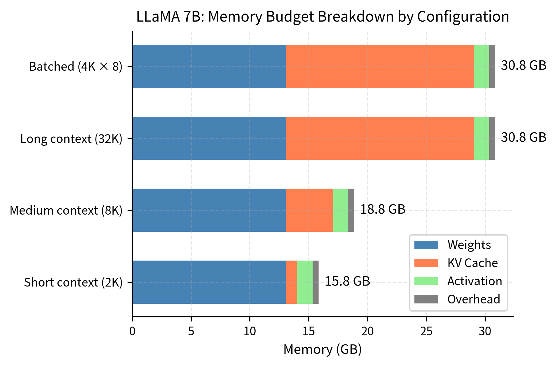
This breakdown demonstrates how dramatically memory requirements shift across different usage patterns. For short 2K contexts, model weights dominate at roughly 85% of total memory, with KV cache representing only about 7% of requirements. As context expands to 32K tokens, the cache grows to consume approximately 35% of total memory, becoming the second-largest component after weights. Similarly, batching 8 sequences at 4K context each shifts the cache to around 30% of total memory. This transition from weight-dominated to cache-dominated memory profiles has profound implications for deployment strategies and hardware selection.

The percentage breakdown reveals how memory allocation shifts with configuration. At short contexts, weights dominate at about 85% of total memory. At long contexts or large batches, the KV cache becomes the primary memory consumer, reaching 35% of total memory. This shift demonstrates why cache optimization becomes critical for long-context applications.

When KV cache memory dominates, we encounter a fundamental constraint: the memory bottleneck, which differs from the compute bottleneck that traditionally limits deep learning. Understanding this distinction is essential because the remedies for each bottleneck are completely different.

In a compute-bound scenario, performance is limited by how fast the GPU can perform arithmetic operations. The solution is to use faster GPUs with more compute units, or to reduce the number of operations through algorithmic improvements. In a memory-bound scenario, performance is limited by how fast data can move between memory and compute units. The GPU sits idle while waiting for data to arrive, regardless of how many arithmetic units it has available. Upgrading to a faster GPU may not improve inference speed if the bottleneck is memory bandwidth.

During token generation, the model performs:

1. Attention computation (memory-bound): Uses cached keys and values. The attention mechanism reads the entire KV cache to compute attention scores, then reads it again to compute the weighted value sum. This requires moving massive amounts of data from GPU memory to compute units.
2. Feed-forward computation (compute-bound): Dense matrix multiplications. The feed-forward layers perform arithmetic-heavy operations where the same weight matrix is applied to the input, allowing high arithmetic intensity.

Modern GPUs have enormous compute capacity (for example, A100 with 312 TFLOPS for FP16) but limited memory bandwidth (for example, A100 with 2 TB/s). The ratio between these capabilities determines the threshold between compute-bound and memory-bound operation. The arithmetic intensity, measured as the number of floating point operations performed per byte of data transferred, determines which resource is the bottleneck. We can formalize this relationship using the roofline model:

where:

• $\mathcal{I}$: the arithmetic intensity (measured in operations per byte)
• $\text{FLOPs}$: the total floating point operations performed
• $\text{Bytes}$: the total data transferred from memory, dominated by KV cache reads

If $\mathcal{I}$ is lower than the GPU's ratio of peak compute to peak bandwidth, the process is memory-bound. For an A100, this threshold is approximately 156 FLOPs per byte (312 TFLOPS divided by 2 TB/s). Operations with lower arithmetic intensity cannot fully utilize GPU compute because they wait for memory transfers.

The practical implication is that for single-sequence generation at typical context lengths, the attention computation is memory-bound. Each token generation requires reading the entire KV cache from memory. This memory transfer takes longer than the actual computation, which is why techniques like FlashAttention and KV cache quantization provide significant speedups without reducing the number of arithmetic operations.

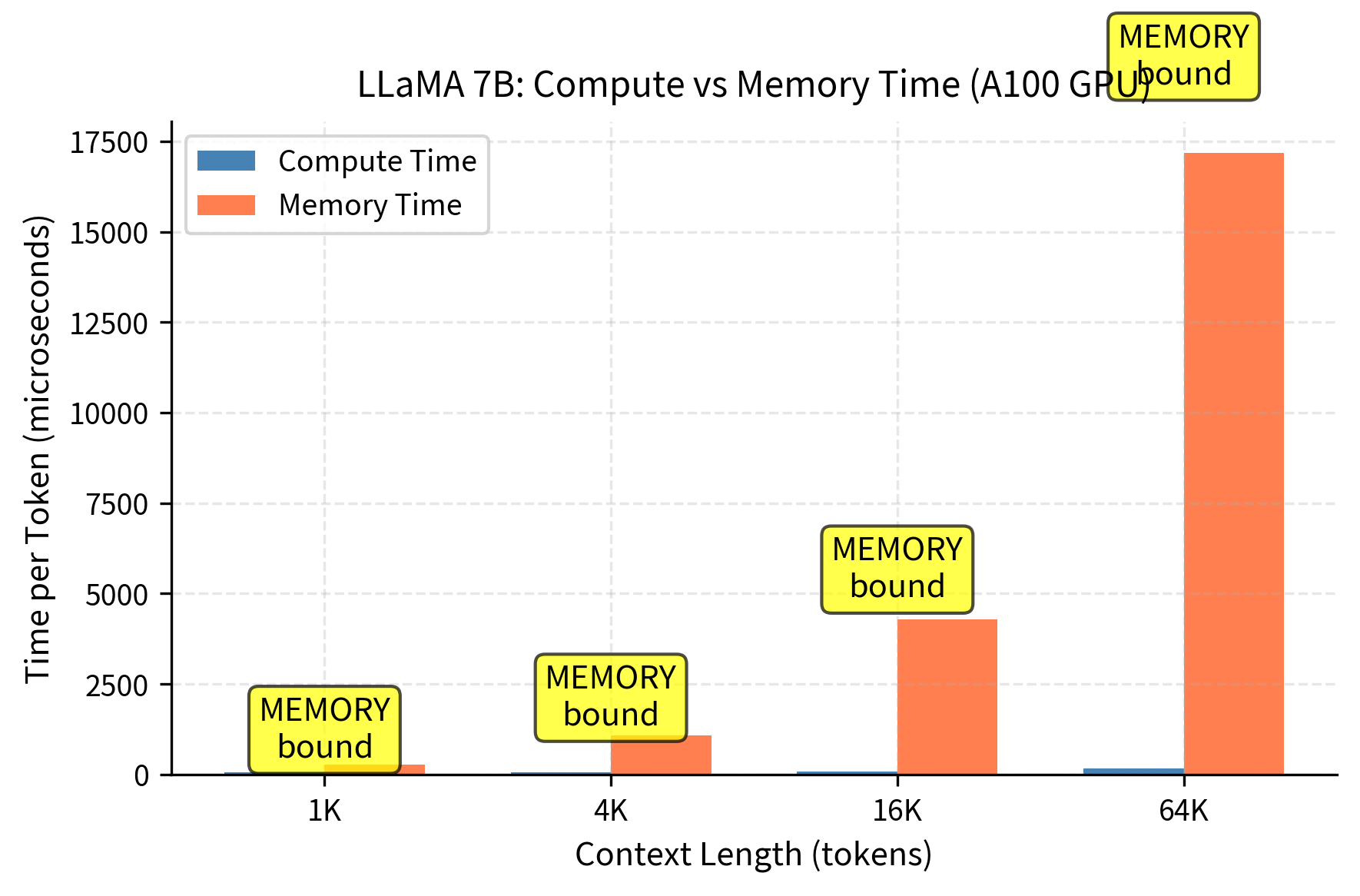
These results reveal a critical pattern in transformer inference performance. At shorter contexts (1K-4K tokens), memory transfer time dominates compute time, indicating the GPU spends more time waiting for KV cache data than actually performing computations. As context length increases to 16K and beyond, the bottleneck shifts toward compute as the sheer number of attention operations grows. However, for typical production scenarios with 4K-8K contexts, memory bandwidth is the primary constraint. This explains why FlashAttention and KV cache quantization provide significant speedups by reducing memory traffic. This bottleneck analysis demonstrates that at reasonable context lengths, single-sequence generation is memory-bound. The GPU spends most of its time waiting for KV cache data to transfer from high-bandwidth memory (HBM) to the compute units. Increasing batch size helps amortize memory transfer costs, but this in turn increases total memory requirements, creating a constrained optimization problem.

Let's visualize how memory allocation differs across model sizes and architectures:

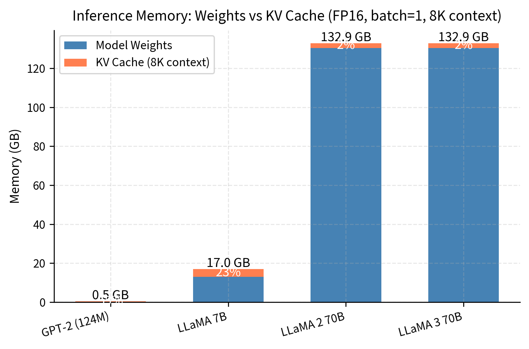
Without GQA, LLaMA 70B would require 8× more KV cache memory, making long-context inference impractical on most hardware. The visualization clearly demonstrates how Grouped Query Attention keeps cache proportions manageable at the 70B scale, with the cache remaining a smaller fraction of total memory compared to what standard MHA would require.

Before deploying a model, estimate memory requirements for your target configuration. Here is a practical workflow:

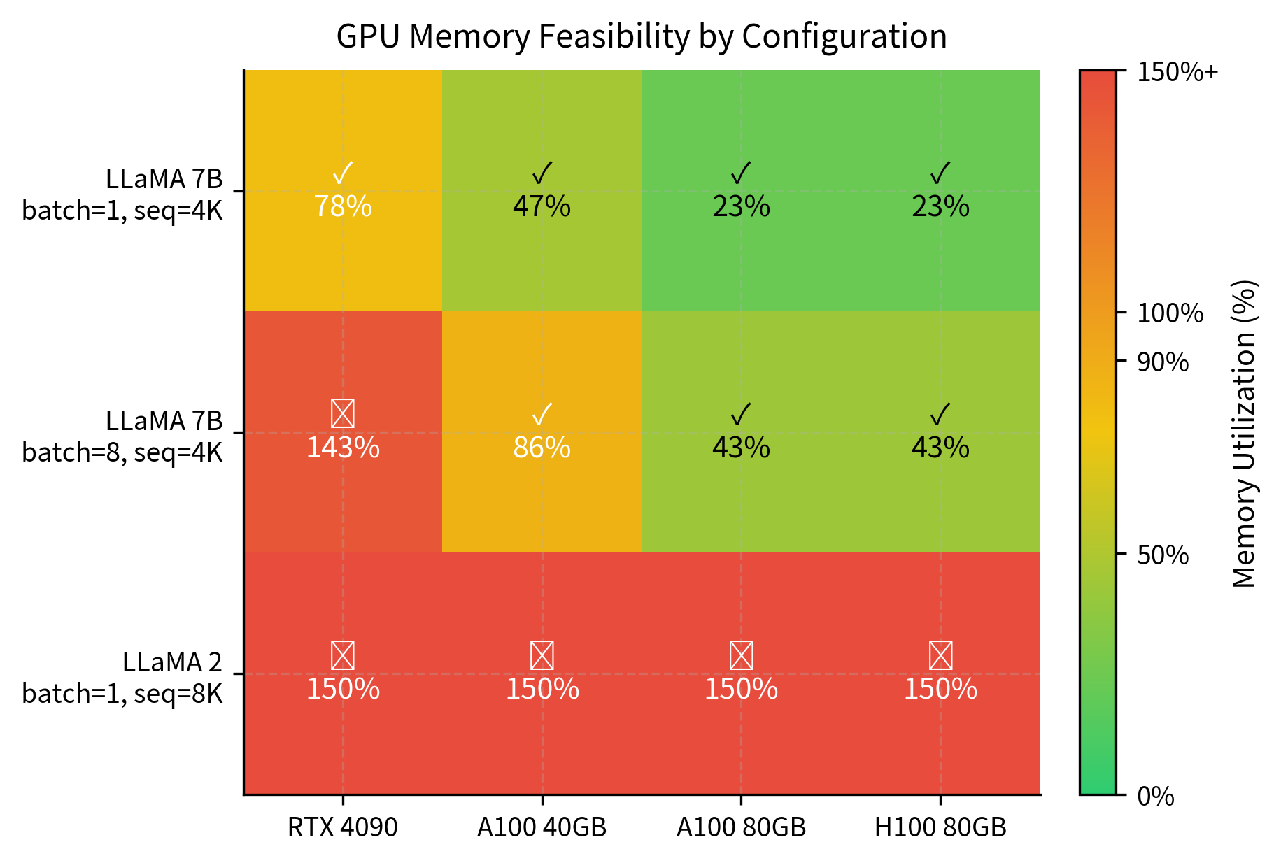
These results illustrate the hardware requirements for different deployment scenarios. LLaMA 7B fits comfortably on all tested GPUs for single-sequence inference at 4K context, with even the 24GB RTX 4090 providing adequate headroom. However, scaling to batch size 8 pushes requirements beyond consumer hardware, requiring datacenter GPUs like the A100. The 70B model at 8K context is borderline even on high-end 80GB GPUs, demonstrating why models of this scale typically require either multi-GPU setups or aggressive optimization techniques like quantization and cache compression. These constraints directly inform deployment decisions: smaller models offer flexibility across hardware tiers, while frontier models demand specialized infrastructure.

The feasibility analysis demonstrates the practical constraints of different GPU configurations. For production deployment, understanding these memory limits is essential for selecting appropriate hardware.

The memory requirements of KV caching create several practical challenges:

• Long context support requires substantial memory investment. A 128K context window for LLaMA 7B requires 32GB of KV cache alone, exceeding most consumer GPU memory. This explains why long-context models often require cloud deployment or specialized hardware.

• Batch size is constrained by available memory. High-throughput serving, handling many concurrent requests, requires either smaller models, shorter contexts, or memory optimization techniques. The tradeoff between latency (single-sequence speed) and throughput (requests per second) is fundamentally a memory allocation problem.

• Linear scaling creates predictable but inflexible costs. Unlike attention computation, where techniques like FlashAttention reduce memory overhead, the KV cache is fundamentally required for correct generation. Every token's keys and values must be stored somewhere.

These constraints have driven significant research into cache optimization. The next chapter explores Paged Attention, which applies virtual memory concepts to manage KV cache more efficiently. Subsequent chapters cover cache compression techniques that reduce memory by quantizing or pruning cached values. Together, these techniques enable longer contexts and larger batches while keeping memory requirements manageable.

The following parameters are essential for KV cache memory calculation:

• num_layers: Number of transformer layers in the model. Each layer maintains its own key and value cache, so cache memory scales linearly with the number of layers.
• num_kv_heads: Number of key-value attention heads, also written as num_KV_heads or $H_{\text{kv}}$. In standard Multi-Head Attention, this equals the number of query heads. Grouped Query Attention uses fewer KV heads to reduce memory.
• head_dim: Dimension of each attention head, also written as $D_h$. Typically 64, 96, or 128. Combined with number of heads, this determines the model dimension.
• batch_size: Number of sequences processed simultaneously. Each sequence maintains its own independent cache, so memory scales linearly with batch size.
• seq_len: Context length in tokens. Cache memory grows linearly as more tokens are processed and cached.
• dtype_bytes: Bytes per element based on data type. FP16/BF16 use 2 bytes, FP32 uses 4 bytes, INT8 uses 1 byte, INT4 uses 0.5 bytes.

KV cache memory follows a simple formula, $2 \times L \times B \times T \times H_{kv} \times D_h \times \text{bytes}$. This linear scaling with batch size and sequence length means the cache can easily exceed model weights for long-context or batched inference.

Key takeaways:

• Model size scales differently than cache size: A 10x larger model does not require 10x more cache when using GQA
• Grouped Query Attention is crucial: LLaMA 2's GQA reduces 70B cache by 8x compared to standard MHA
• Long contexts are memory-expensive: At 32K or more tokens, KV cache typically exceeds model weight memory
• Generation is memory-bound: GPU compute utilization is limited by memory bandwidth when reading cached keys and values
• Deployment planning requires careful calculation: Before serving a model, estimate total memory including weights, cache, and overhead

Understanding these memory dynamics is essential. The cache size calculator provides a foundation for capacity planning. The bottleneck analysis explains why memory optimization techniques, covered in upcoming chapters, are critical for efficient inference.

Ready to test your understanding? Take this quick quiz to reinforce what you've learned about KV cache memory requirements and deployment planning.