

Explore DPO variants including IPO, KTO, ORPO, and cDPO. Learn when to use each method for LLM alignment based on data format and computational constraints.

This article is part of the free-to-read Language AI Handbook
Choose your expertise level to adjust how many terms are explained. Beginners see more tooltips, experts see fewer to maintain reading flow. Hover over underlined terms for instant definitions.
DPO Variants
In the previous chapters, we derived Direct Preference Optimization from first principles and implemented it as a simpler alternative to RLHF. While DPO represented a significant advance in alignment methodology, you quickly identified several limitations: sensitivity to noisy preference labels, the requirement for paired preference data, potential overfitting to extreme probability ratios, and the computational overhead of maintaining a frozen reference model. These challenges motivated a wave of DPO variants, each addressing specific weaknesses while preserving the core insight that preference learning can bypass explicit reward modeling.
This chapter explores the most influential DPO variants: IPO addresses overfitting through a regularized objective, KTO enables learning from unpaired binary feedback, ORPO eliminates the reference model entirely, and cDPO handles label noise through conservative smoothing. Understanding these variants equips you to select the right alignment method for your data characteristics and computational constraints.
Identity Preference Optimization (IPO)
IPO emerged from a careful analysis of DPO's theoretical properties. Azar et al. (2024) identified a subtle but important issue: as DPO training progresses, the implicit reward gap between chosen and rejected responses can grow unboundedly, causing the policy to assign extreme probabilities that don't reflect the actual strength of human preferences.
The Overfitting Problem in DPO
To understand why IPO was developed, we must first examine a fundamental tension within DPO's optimization dynamics. Recall from our DPO derivation that the loss function is:
where:
- : the DPO loss function
- : the expectation over the dataset of preference pairs
- : the probability of response given prompt under the policy being trained
- : the probability under the frozen reference model
- : the chosen (winner) and rejected (loser) responses
- : the temperature parameter controlling the strength of the KL divergence penalty
- : the sigmoid function
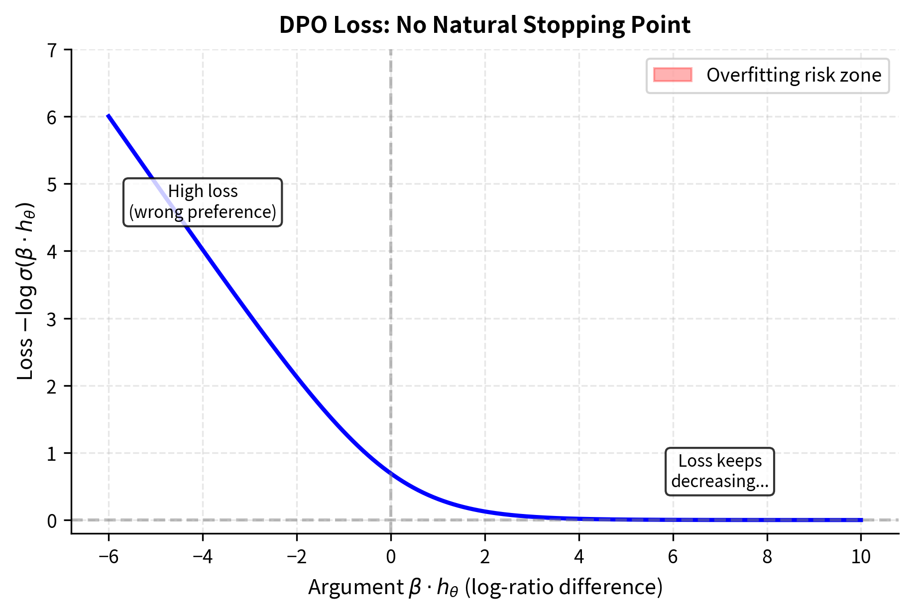
To appreciate the overfitting problem, consider what this loss function is asking the model to do. The expression inside the sigmoid represents the difference between two log-ratios: how much more likely the policy makes the chosen response compared to the reference, minus the same quantity for the rejected response. The negative log-sigmoid of this quantity becomes the loss. When training minimizes this loss, it maximizes what's inside the log-sigmoid.
The sigmoid function approaches 1 as its argument grows large. To minimize this loss (maximize the log), the model is incentivized to make the log-ratio difference as large as possible. In the limit, this pushes the model toward assigning probability approaching 1 to chosen responses and probability approaching 0 to rejected ones. There is no natural stopping point in this formulation: the gradient always points toward making the gap larger, even when the gap is already enormous.
This behavior is problematic for several reasons:
- Overconfidence: Human preferences aren't absolute. A response labeled "chosen" isn't infinitely better than the "rejected" alternative; it's merely preferred in that comparison. Two responses might differ only slightly in quality, yet the labeling treats one as definitively better. When the model learns to assign extreme probabilities based on these labels, it develops a false sense of certainty that doesn't match the underlying reality of human judgment.
- Training instability: As log probabilities approach for rejected responses, gradients can become unstable. The model must push probability mass away from rejected responses, and when those probabilities become vanishingly small, the numerical representations become problematic. Small perturbations can cause large swings in the loss.
- Poor generalization: Overfitting to training preferences may not transfer to held-out prompts. When the model learns extreme preferences on training data, it essentially memorizes that specific responses are "infinitely good" or "infinitely bad" rather than learning generalizable patterns about what makes responses better or worse.
IPO's Squared Error Objective
IPO addresses this by reformulating preference learning as a regression problem with a specific target. The key insight is that instead of allowing the reward gap to grow without bound, we should specify how large we want that gap to be and then train the model to achieve exactly that target. This transforms an unbounded optimization problem into a bounded one with clear convergence criteria.
Instead of pushing the reward gap to infinity, IPO targets a fixed margin:
where:
- : the IPO loss function
- : the expectation over the dataset of preference pairs
- : the target margin derived from the regularization strength
- : the policy and reference models
The key innovation is the squared loss with target . This creates fundamentally different optimization dynamics. Rather than rewarding the model for making the gap as large as possible, IPO rewards the model for making the gap equal to a specific value. Any deviation from this target, whether too small or too large, incurs a penalty. This is the essence of regression: we have a target value, and we minimize the squared distance to that target.
To analyze these dynamics more precisely, let's define the log-ratio difference as:
where:
- : the difference in log-probability ratios between chosen and rejected responses
- : the "implicit reward" for a specific response
This quantity captures the essence of what preference optimization is trying to achieve. It measures how much the policy has learned to prefer the chosen response over the rejected one, relative to what the reference model would predict. A positive value means the policy has shifted probability mass toward the chosen response; a larger positive value means a stronger learned preference.
With this notation, the IPO loss becomes elegantly simple:
where:
- : the IPO loss function
- : the expectation over the dataset
- : the log-ratio difference computed by the model
- : the specific target value that the difference should converge to
This formulation makes the regression nature of IPO crystal clear. We are asking the model to make equal to for every preference pair in the dataset. The squared loss penalizes deviations in either direction: if the model hasn't learned a strong enough preference (), the loss is positive and gradients push toward a larger gap; if the model has learned too strong a preference (), the loss is also positive and gradients push toward a smaller gap.
The gradient with respect to reveals this self-correcting behavior:
where:
- : the gradient of the loss with respect to the log-ratio difference
- : the error term (distance from target) that drives the update
This gradient is zero when , creating a stable equilibrium. Once the log-ratio difference reaches the target margin, there's no further pressure to increase it. This bounded optimization prevents the extreme probability assignments that plague standard DPO. The equilibrium is not just stable but attractive: regardless of where training starts, the gradients always point toward the target, and the strength of the gradient is proportional to the distance from the target.
Interpreting the Target Margin
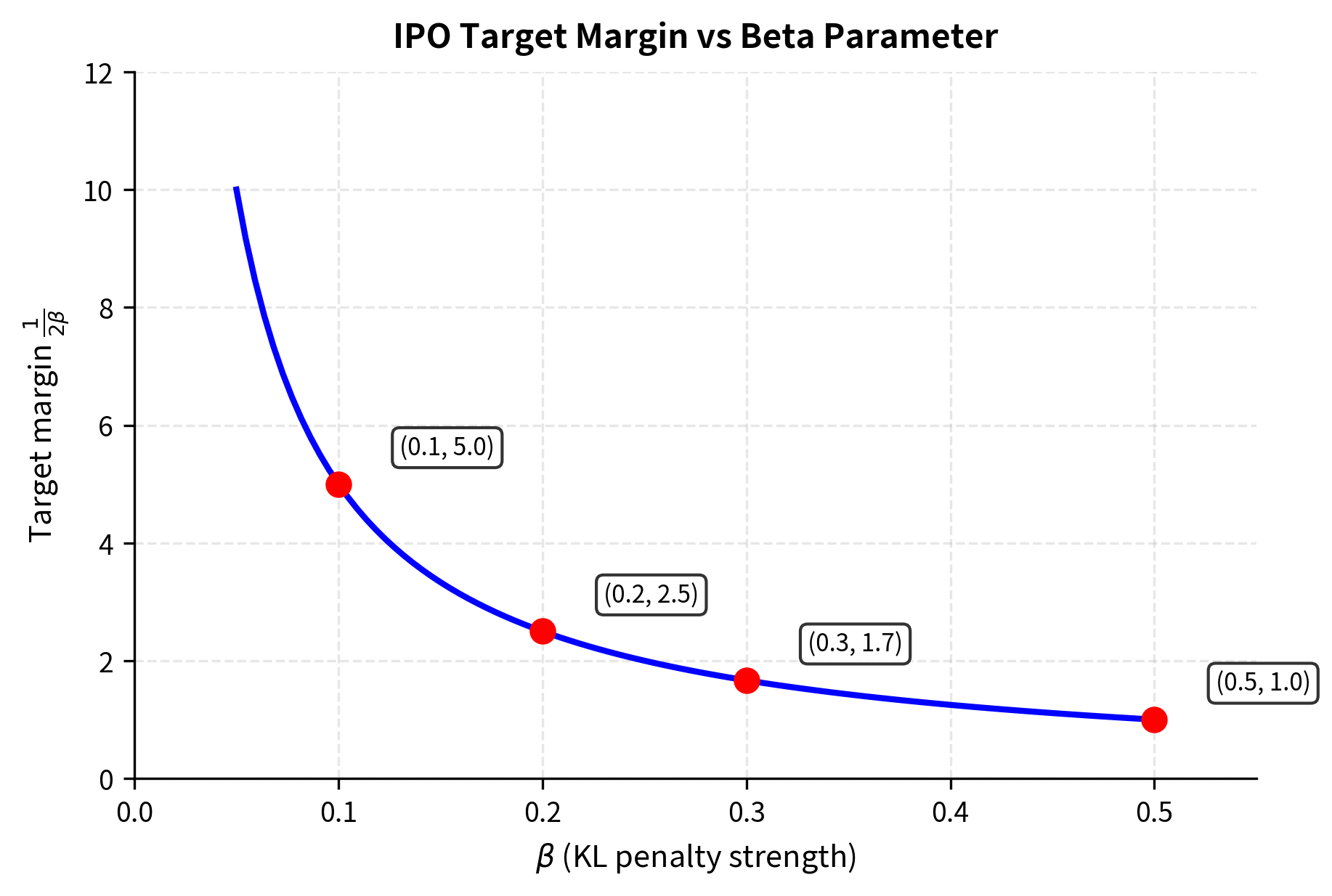
The target has a principled interpretation that connects IPO back to the theoretical foundations of preference learning. The parameter controls the strength of the KL constraint (as discussed in Part XXVII, Chapter 10). A larger means weaker regularization, allowing larger deviations from the reference policy. With IPO's target:
- When is large (weak KL penalty), the target margin is small
- When is small (strong KL penalty), the target margin is large
This might seem counterintuitive until you consider that IPO's margin represents how much the policy should diverge from the reference on each preference pair. Stronger KL constraints ( small) actually permit larger per-example margins because the overall deviation is more tightly controlled. To understand this, think about a budget analogy: if you have a strict overall spending limit, you can afford to splurge on individual items because you're being careful everywhere else. Conversely, if you have a loose overall limit, you need to be more conservative on each purchase to avoid overshooting.
The target margin also has an interpretation in terms of the Bradley-Terry model that underlies preference learning. In this model, the probability that response is preferred to depends on the difference in their rewards. The target corresponds to a specific preference probability that represents a moderate preference rather than absolute certainty. This aligns with the reality that human annotations express preferences, not certainties.
Gradient Comparison
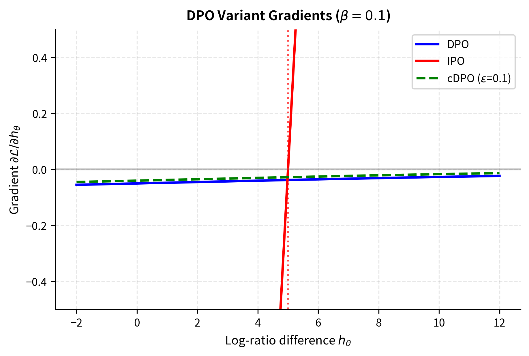
Different loss functions result in different gradient behaviors, explaining why methods perform differently in practice. The gradient determines how the model updates its parameters at each step, so differences in gradient behavior translate directly into differences in training dynamics.
DPO gradient magnitude:
where:
- : the temperature parameter
- : the sigmoid of the negative scaled log-ratio, acting as a weighting factor
This sigmoid term means DPO's gradient is largest when is near zero (uncertain predictions) and vanishes as (confident predictions). The intuition here is that DPO pushes hardest when the model is uncertain about which response is preferred, and pushes more gently when the model is already confident. While vanishing gradients prevent infinite growth in principle, they also mean learning slows dramatically once the model becomes confident. This creates a problematic dynamic: the model can still drift toward extreme probabilities because the gradients, though small, remain consistently positive.
IPO gradient magnitude:
where:
- : the absolute distance from the target margin
IPO's gradient magnitude is proportional to distance from the target. If the model overshoots the target (), the gradient pushes it back. This self-correcting behavior is absent in DPO. The gradient grows stronger as the model strays further from the target, which means that even large deviations are corrected rather than allowed to persist. This property makes IPO training more robust to initialization and hyperparameter choices, since the optimization will eventually find the target regardless of where it starts.
Kahneman-Tversky Optimization (KTO)
While DPO and IPO improve upon RLHF's computational complexity, they share a fundamental data requirement: paired preferences. Each training example must contain a prompt with both a chosen and rejected response. This pairing constraint creates practical challenges.
The Unpaired Feedback Problem
Real-world human feedback often comes in unpaired form, and this mismatch between how feedback is collected and how preference optimization algorithms expect data creates significant friction in practical applications:
- Binary ratings: You click thumbs up or thumbs down on individual responses
- Flagging systems: You report problematic outputs without providing alternatives
- Implicit signals: Engagement metrics indicate whether a response was helpful
Converting this abundant unpaired feedback into DPO's paired format requires either discarding data or artificially constructing pairs. Discarding data wastes valuable signal; constructing pairs introduces artifacts that may not reflect genuine preferences. Consider a scenario where you have 10,000 thumbs-up ratings and 5,000 thumbs-down ratings, but these ratings come from different conversations with different prompts. To use DPO, you would need to either match these into pairs somehow, losing most of your data, or generate new responses to create artificial comparisons.
KTO, introduced by Ethayarajh et al. (2024), eliminates this requirement by designing an objective that works directly with unpaired binary feedback. This enables learning from the full breadth of available feedback without forcing it into an unnatural format.
Inspiration from Prospect Theory
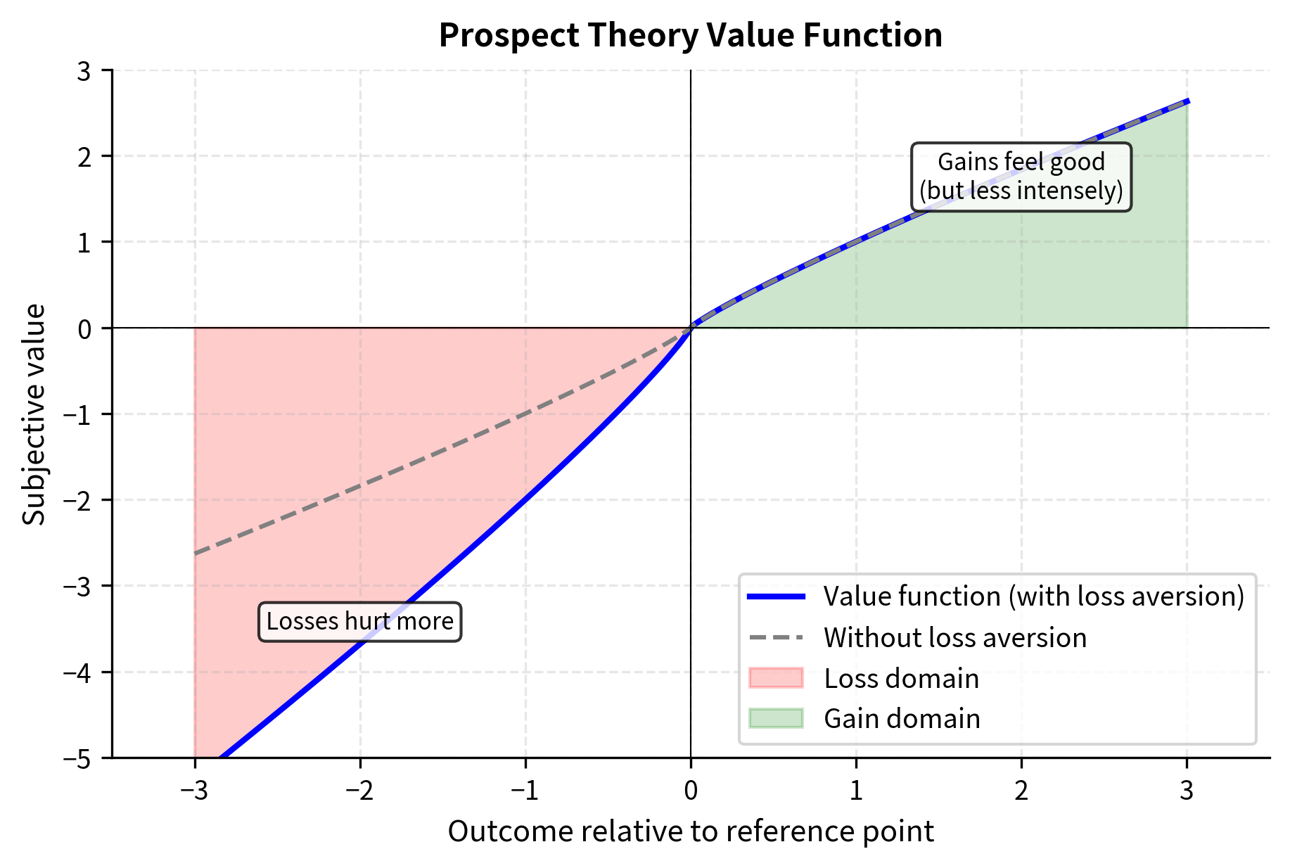
KTO draws inspiration from Kahneman and Tversky's prospect theory, which describes how humans actually make decisions under uncertainty. This connection to behavioral economics is more than a naming convention: it provides principled guidance for how to weight different types of feedback. Two key insights from behavioral economics inform KTO's design:
Reference dependence: People evaluate outcomes relative to a reference point, not in absolute terms. A $100 gain feels different depending on whether you expected $0 or $200. This insight suggests that the "goodness" of a model response should be measured relative to some baseline expectation, not in absolute terms. A response that seems mediocre after an excellent previous response might seem impressive after a poor one.
Loss aversion: Losses loom larger than equivalent gains. Losing $100 feels worse than gaining $100 feels good. Empirically, losses are weighted approximately 2x more heavily than gains. For alignment, this suggests that avoiding bad outputs might be more important than producing good ones. You might forgive a bland response, but you remember harmful or incorrect ones.
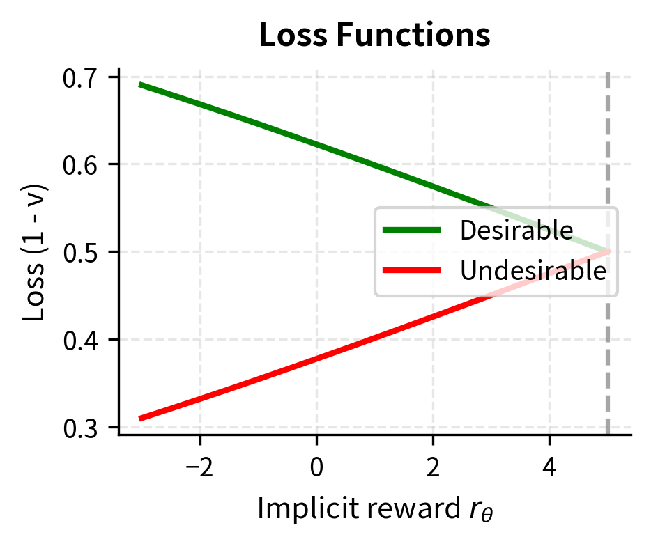
KTO incorporates both principles into its loss function, treating "desirable" and "undesirable" responses asymmetrically.
The KTO Loss Function
The construction of KTO's loss function proceeds in several stages, each motivated by the behavioral economics principles described above. We begin by defining the implicit reward, which serves as the raw signal that KTO will transform into a learning objective.
For a response to prompt with binary label , KTO defines:
where:
- : the implicit reward assigned to response given prompt
- : the probability of the response under the current policy
- : the probability of the response under the reference model
This is the implicit reward, the same quantity used in DPO. It measures how much more likely the current policy makes this response compared to the reference. A positive implicit reward means the policy has learned to favor this response; a negative implicit reward means the policy has learned to disfavor it. The key insight is that this quantity is well-defined even for a single response, without needing a comparison partner.
KTO then defines a reference point that implements the reference dependence principle from prospect theory:
where:
- : the reference point (baseline) for evaluation
- : the policy and reference models
- : the training dataset distribution
- : the expectation over prompts sampled from
- : the Kullback-Leibler divergence measuring the drift of the policy from the reference
The reference point represents the expected KL divergence between policy and reference across the training distribution. In practice, this is estimated from a running average during training. The reference point serves a crucial role: it defines what counts as "above average" versus "below average" performance. Rather than using an arbitrary fixed threshold, KTO adapts the reference point to the current state of training, creating a dynamic baseline that evolves as the model improves.
With the implicit reward and reference point defined, KTO constructs a value function that differs based on whether the response is desirable:
where:
- : the value assigned to the response, bounded between 0 and 1
- : the sigmoid function
- : the label indicating if the response is desirable or undesirable
- : the shifted implicit reward used for desirable examples
This asymmetric definition is the mathematical implementation of reference dependence. For desirable responses, we ask: is the implicit reward higher than the reference point? For undesirable responses, we ask: is the implicit reward lower than the reference point? The sigmoid function squashes these comparisons into the range (0, 1), creating a smooth value measure.
The loss weights desirable and undesirable examples differently, implementing the loss aversion principle:
where:
- : the KTO loss function
- : the expectation over the dataset of labeled examples
- : the weighting factor specific to the label type
- : the value computed by the value function
Where and , typically with to implement loss aversion. By setting , we tell the model that failing to suppress a bad response is worse than failing to promote a good response. This asymmetry reflects the empirical finding that you are more bothered by failures than impressed by successes.
Understanding the Value Function
The asymmetric value function encodes prospect theory's core insights, and understanding its behavior illuminates why KTO works. The function transforms implicit rewards into values differently depending on the label, creating distinct learning signals for positive and negative feedback.
For desirable responses, the sigmoid argument is . The model is rewarded (low loss) when the implicit reward exceeds the reference point. Intuitively, the model should push desirable responses to have higher implicit rewards than average. When , the sigmoid output is greater than 0.5, meaning the value is high and the loss is low. The model learns to associate desirable responses with above-average implicit rewards.
For undesirable responses, the sigmoid argument is . The model is rewarded when the implicit reward falls below the reference point. The model should push undesirable responses to have lower implicit rewards than average. When , the sigmoid output is greater than 0.5, meaning the value is high and the loss is low. The model learns to associate undesirable responses with below-average implicit rewards.
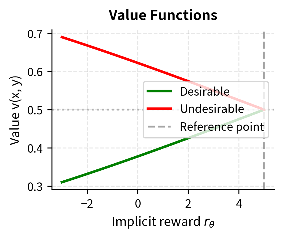
The reference point serves as the dividing line between "gains" (implicit rewards above average) and "losses" (implicit rewards below average). This relative framing means KTO doesn't need paired comparisons; it learns to push good responses up and bad responses down relative to an adaptive baseline. The elegance of this approach is that it converts an inherently comparative problem (which response is better?) into a classification problem (is this response good or bad?), which is exactly the form that unpaired feedback provides.
Practical Implementation Details
KTO requires tracking the reference point during training:
The running average KL is typically computed as:
KTO's Advantages
KTO offers several practical benefits:
- Data efficiency: Uses all available binary feedback without discarding unpaired examples
- Natural data format: Matches how most user feedback is actually collected
- Principled asymmetry: The loss-aversion weighting reflects empirical findings about human judgment
- Stable training: The reference point provides a grounding mechanism similar to IPO's target
Odds Ratio Preference Optimization (ORPO)
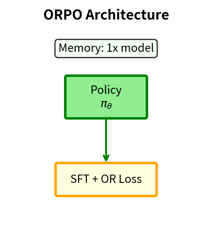
ORPO takes a more radical departure from the DPO framework by eliminating the reference model entirely. Introduced by Hong et al. (2024), ORPO combines supervised fine-tuning with preference optimization into a single training objective.
Motivation: The Reference Model Burden
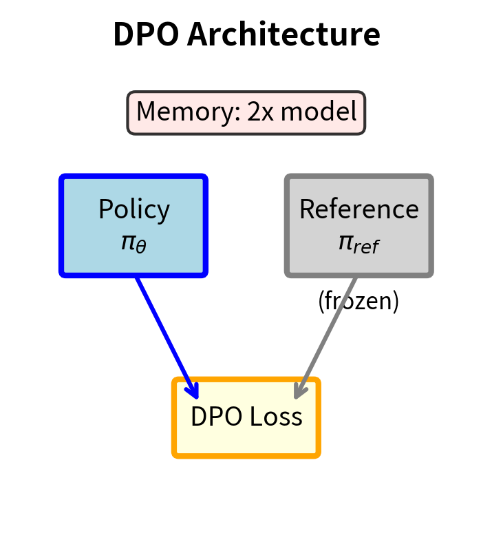
All previous methods (RLHF, DPO, IPO, KTO) require maintaining a reference policy . This creates practical complications:
- Memory overhead: Two copies of the model must reside in memory (or frequent loading/unloading)
- Two-stage training: Models typically undergo SFT first to create the reference, then preference training
- Computational cost: Every forward pass requires evaluating both policies
ORPO asks: can we eliminate the reference model while still preventing the policy from drifting arbitrarily far from sensible outputs?
The Odds Ratio Approach
Instead of comparing log probabilities to a reference, ORPO uses the odds ratio between chosen and rejected responses within the current policy itself. This shift is significant. Instead of measuring change from a fixed reference, ORPO measures the relative likelihood of responses within the current policy. The odds of generating response given prompt are:
where:
- : the odds of generating response under policy
- : the probability of the response
The odds representation has a natural interpretation: it tells us how likely the response is compared to everything else. If the odds are 2:1, the response is twice as likely as all alternatives combined. The odds formulation is particularly useful because ratios of odds have clean mathematical properties, as we will see shortly.
For a language model, the probability of a specific sequence becomes numerically insignificant as length increases, making direct odds calculation unstable. Consider that even a moderately long sequence might have a probability of or smaller, which would make both the numerator and denominator of the odds calculation problematically small. ORPO instead defines the sequence-level odds as the geometric mean of the token-level odds:
where:
- : the input prompt
- : the length of the response in tokens
- : the token at step
- : the sequence of tokens preceding step (the context)
- : the probability of the next token given the prompt and previous tokens
- : the exponentiation to convert average log-odds back to the odds scale
This formulation works at the token level, where probabilities are large enough to be numerically stable, and then aggregates these token-level odds into a sequence-level measure. The averaging by sequence length ensures that longer sequences aren't automatically penalized, since we're taking a geometric mean rather than a product.
The ratio of odds between chosen () and rejected () responses becomes:
where:
- : the odds ratio between the chosen and rejected responses
- : the chosen and rejected responses
This odds ratio captures the relative preference of the current policy for the chosen response over the rejected one. An odds ratio greater than 1 means the policy favors the chosen response; we want to train the policy to increase this ratio.
The ORPO Loss Function
ORPO combines two components that work together to provide both language modeling signal and preference signal. This combination is what allows ORPO to eliminate the separate SFT stage and the reference model.
- Supervised fine-tuning loss on the chosen response:
where:
- : the supervised fine-tuning loss component
- : the expectation over prompts and chosen responses
- : the likelihood of the chosen response
This component serves two purposes: it teaches the model to generate fluent, coherent text (the standard language modeling objective), and it provides an anchor that prevents the model from drifting too far from producing sensible outputs. By training on the chosen responses, the model learns what good outputs look like.
- Odds ratio loss that increases the relative odds of chosen over rejected:
where:
- : the odds ratio loss component
- : the expectation over the dataset of preference pairs
- : the chosen and rejected responses
- : the log odds ratio (log of the ratio of odds)
- : the sigmoid function
This component implements the preference learning objective. By maximizing the log-sigmoid of the log odds ratio, we push the model to make the chosen response relatively more likely than the rejected one. The structure is similar to DPO's loss, but operates on odds ratios within a single policy rather than log-probability ratios between two policies.
The combined ORPO objective is:
where:
- : the total ORPO loss
- : the coefficient weighting the odds ratio loss against the SFT loss
The hyperparameter controls the trade-off between learning to generate good responses and learning to distinguish good responses from bad ones. Too small a and the model ignores preferences; too large and the model may sacrifice fluency for preference optimization.
Why Odds Ratios Work
The odds ratio formulation provides implicit regularization without an explicit reference model. To understand why this works, consider what happens during training:
- The SFT loss pulls the model toward generating the chosen response
- The OR loss pushes chosen odds higher relative to rejected odds
- Both losses operate on the same policy, creating a coupled optimization
The key insight is that increasing odds for chosen responses while decreasing odds for rejected responses automatically constrains how much the model can deviate from generating coherent text. If the model tried to maximize the odds ratio by assigning near-zero probability to rejected responses, the SFT loss on chosen responses would suffer because probability mass must be conserved. The model cannot simply declare everything "bad"; it must maintain a coherent probability distribution over all possible responses.
This coupling between the two loss components creates an implicit regularization effect. The SFT loss ensures the model keeps generating reasonable text, while the OR loss ensures it prefers better text to worse text. Neither loss alone would achieve both objectives, but together they provide a balanced training signal.
Comparing Log-Ratio and Odds-Ratio Objectives
Comparing what DPO and ORPO optimize reveals how they prevent policy drift.
DPO optimizes:
where:
- : the policy and reference model probabilities
- : the chosen and rejected responses
ORPO optimizes:
where:
- : the log-odds of a response under the current policy
- : the chosen and rejected responses
DPO measures how much the policy's preference for over has changed relative to the reference. ORPO measures the absolute odds ratio within the current policy. The reference model in DPO serves as an anchor; ORPO's SFT component and odds formulation provide an alternative form of anchoring. In DPO, the anchor is external: a frozen copy of the model from before preference training. In ORPO, the anchor is internal: the requirement that the model maintain coherent probability distributions while also producing high-likelihood chosen responses.
Conservative DPO (cDPO)
The variants discussed so far address algorithmic limitations. cDPO, introduced by Mitchell et al. (2023), addresses a data quality issue: label noise in preference annotations.
Label Noise in Preference Data
Human preference annotations are inherently noisy. Annotators may:
- Disagree with each other on the same comparison
- Make mistakes due to fatigue or inattention
- Apply inconsistent criteria across examples
- Be influenced by surface features rather than actual quality
Studies of inter-annotator agreement on preference tasks typically show agreement rates of 70-80%, meaning 20-30% of labels may be "wrong", in the sense that a different annotator would have labeled them oppositely.
Standard DPO treats all preference labels as ground truth. If the training data says , the model learns to prefer . When this label is actually wrong, the model learns an incorrect preference.
Label Smoothing for Preferences
cDPO applies label smoothing to preference labels. The idea behind label smoothing is familiar from classification: instead of training on hard targets (0 or 1), we train on soft targets that acknowledge uncertainty. For preferences, instead of treating each comparison as a certainty, we model the possibility that the annotation might be wrong.
Instead of treating preferences as deterministic (), cDPO models uncertainty:
where:
- : the label smoothing parameter, , representing uncertainty about annotation correctness
The parameter represents our belief about how often the annotations are wrong. If , we trust all annotations completely, recovering standard DPO. If , we believe that 30% of the time, the annotators got it backwards and the rejected response was actually better.
The cDPO loss modifies the Bradley-Terry model probability accordingly:
where:
- : the cDPO loss function
- : the expectation over the dataset
- : the log-ratio difference between chosen and rejected responses
- : the label smoothing parameter
- : the sigmoid function
- : the temperature parameter
This loss function has two terms. The first term, weighted by , is the standard DPO loss: it rewards the model for preferring the labeled chosen response. The second term, weighted by , is the opposite: it rewards the model for preferring the labeled rejected response. The combination represents the expected loss under our belief about annotation accuracy.
Using the identity , we can rewrite this loss to explicitly show the probability mass assigned to the rejected response:
where:
- : the probability assigned to the rejected response (equivalent to )
- : the weighting factor for the "incorrect" preference direction
Effect on Optimization
Label smoothing fundamentally changes the loss landscape. The gradient of cDPO with respect to is:
where:
- : the gradient of the loss with respect to the log-ratio difference
This gradient has two competing terms. The first term pushes toward larger (stronger preference for chosen). The second term pushes toward smaller (acknowledging that the rejected response might actually be better). These competing forces create a balance point where the gradient is zero.
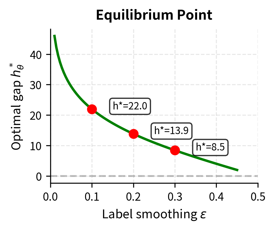
Setting the gradient to zero allows us to solve for the optimal log-ratio difference :
where:
- : the optimal value of the log-ratio difference
- : the label smoothing parameter
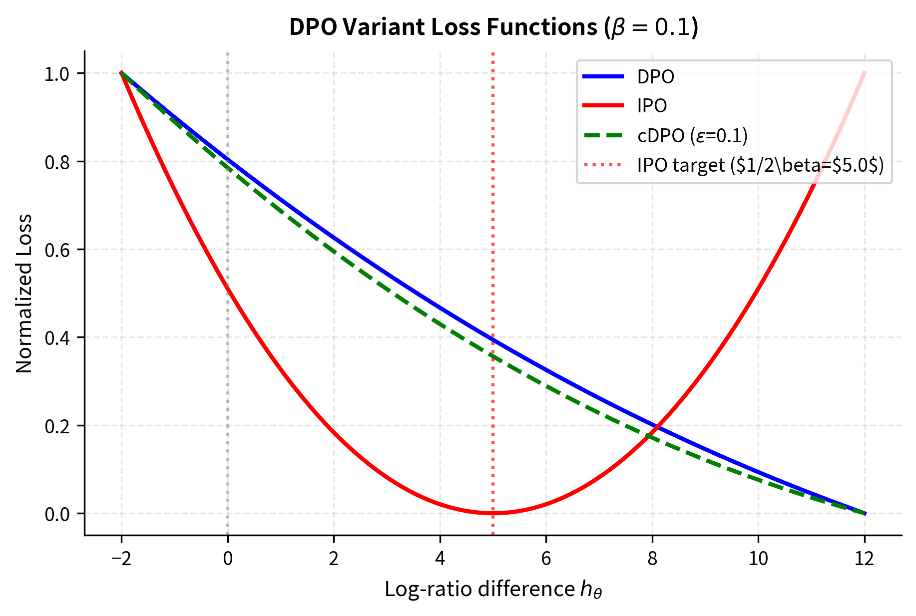
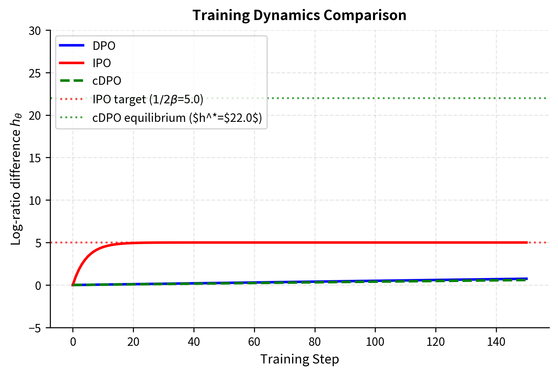
This means cDPO has a finite optimal gap (similar to IPO), which depends on . With standard DPO (), the optimal gap is infinite. With cDPO (), the model converges to a bounded preference strength. The relationship between and the optimal gap is intuitive: higher annotation uncertainty (larger ) leads to a smaller optimal gap, because the model shouldn't be confident when the labels might be wrong.
Choosing the Smoothing Parameter
The smoothing parameter should reflect actual annotation noise. Practical guidelines include:
- : Assumes 90% annotation accuracy, appropriate for high-quality curated datasets
- : Assumes 80% accuracy, appropriate for crowd-sourced annotations
- : Assumes 70% accuracy, appropriate for noisy or automated annotations
When inter-annotator agreement data is available, can be estimated directly as the disagreement rate.
Implementation Comparison
Let's implement all four variants to see the differences in practice.
Now let's implement KTO and ORPO, which have different data requirements:
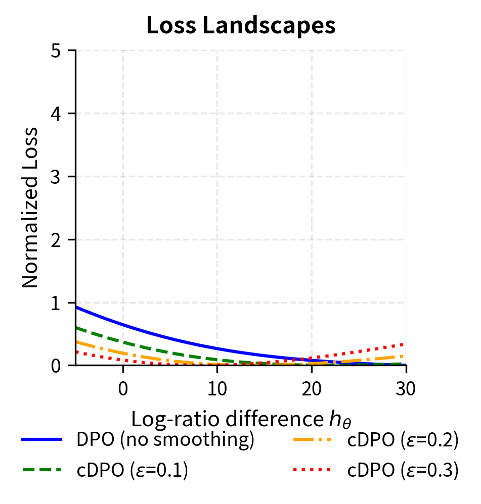
Let's visualize how these losses behave differently:
Now let's examine the gradients:
Comparing Alignment Methods
With multiple alignment approaches now available, selecting the right method depends on your specific constraints: data format, computational budget, annotation quality, and desired training dynamics.
Decision Framework
The choice between alignment methods depends on several factors:
Data format availability:
- Paired preferences (chosen vs rejected for same prompt): Use DPO, IPO, cDPO, or ORPO
- Unpaired binary feedback (thumbs up/down on individual responses): Use KTO
- Ranked lists with multiple responses per prompt: DPO can be adapted with pairwise comparisons
Reference model constraints:
- Can maintain frozen reference in memory: DPO, IPO, cDPO, KTO
- Memory-constrained single-model training: ORPO
Annotation quality:
- High-quality expert annotations (>90% consistency): Standard DPO
- Moderate-quality annotations (70-90%): cDPO with appropriate ε
- Noisy or automated labels (<70%): cDPO with higher ε, or KTO
Training stability requirements:
- Need bounded optimization: IPO or cDPO
- Standard training sufficient: DPO

Empirical Performance Comparison
Published results show that no single method dominates across all benchmarks. General patterns from the literature include:
DPO remains a strong baseline. Its simplicity and well-understood behavior make it the default choice for many applications. Performance degradation typically occurs only with very long training or highly noisy data.
IPO shows advantages when training for many epochs or when the preference data has high confidence (strong agreement between responses). The bounded optimization prevents the overconfident predictions that can emerge with extended DPO training.
KTO achieves comparable performance to DPO when preference data is artificially unpaired from originally paired data. When working with naturally unpaired data (binary ratings), KTO significantly outperforms naive approaches like converting to paired format.
ORPO reduces computational overhead by 20-30% by eliminating the reference model. Quality results are competitive with DPO on standard benchmarks, though some studies report slightly lower performance on challenging alignment tasks.
cDPO provides consistent improvements over standard DPO when annotation noise is known to be present. The gains are proportional to the actual noise level; cDPO shows little difference from DPO on clean data.
Computational Costs
The computational characteristics differ significantly:
| Method | Memory | Forward Passes | Training Stages |
|---|---|---|---|
| DPO | 2× model | 2× per step | SFT → DPO |
| IPO | 2× model | 2× per step | SFT → IPO |
| cDPO | 2× model | 2× per step | SFT → cDPO |
| KTO | 2× model | 2× per step | SFT → KTO |
| ORPO | 1× model | 1× per step | Single stage |
ORPO's single-stage training can reduce wall-clock time by 40-50% compared to two-stage approaches, making it attractive for rapid iteration.
Training Dynamics
Let's simulate training dynamics for each method to see how they converge differently:
Practical Guidelines
Based on the analysis above, here are practical recommendations for choosing and implementing DPO variants.
Method Selection Checklist
When selecting an alignment method, consider:
-
What data do you have?
- Paired preferences → DPO, IPO, cDPO, or ORPO
- Unpaired binary feedback → KTO
-
How much memory can you allocate?
- Can fit two models → Any method
- Limited to one model → ORPO
-
How clean are your labels?
- High quality (>90% agreement) → DPO or IPO
- Moderate quality (70-90%) → cDPO with ε ≈ 0.1-0.2
- Low quality (<70%) → cDPO with ε ≈ 0.2-0.3
-
How long will you train?
- Short training (1-3 epochs) → DPO
- Extended training → IPO or cDPO
Hyperparameter Recommendations
Each method has specific hyperparameter considerations:
DPO: The β parameter typically works well in the range 0.1-0.5. Lower values allow more deviation from the reference; higher values keep the policy closer to the reference. Start with β=0.1 and adjust based on whether outputs are too conservative (increase β) or too different from base model (decrease β).
IPO: Uses the same β parameter, but interpretation differs slightly. The target margin 1/2β means smaller β creates larger targets. Start with β=0.1 (target=5) and adjust if convergence is too slow (increase β) or produces weak preferences (decrease β).
cDPO: Choose ε based on estimated annotation noise. If unknown, start with ε=0.1 as a conservative default. The effective training signal strength is (1-2ε), so ε=0.3 reduces effective signal by 60%.
KTO: The loss aversion ratio λ_u/λ_d is typically set to 1.0-2.0. Higher ratios emphasize avoiding bad outputs over producing good ones. The KL reference running average uses momentum 0.9-0.99.
ORPO: The λ_or weight balances SFT and preference objectives. Values of 0.1-0.5 are typical. Too low ignores preferences; too high destabilizes SFT.
Common Pitfalls
Several issues frequently arise when implementing DPO variants:
Length bias: All preference methods can develop biases toward response length if chosen responses are systematically longer or shorter. Monitor average response lengths during training and consider length normalization.
Mode collapse: Aggressive preference optimization can cause the model to produce repetitive outputs. The KL penalty (explicit in RLHF, implicit in DPO) helps, but monitoring diversity metrics is still important.
Reward hacking: As we discussed in Part XXVII, Chapter 5, models can learn to exploit artifacts in preference data. Regular evaluation on held-out prompts helps detect this.
Training instability: Large learning rates combined with small β can cause instability in DPO. Start with learning rates an order of magnitude smaller than SFT and increase gradually.
Limitations and Impact
The proliferation of DPO variants reflects both the importance of alignment and the difficulty of getting it right. Each method addresses real limitations, but none fully solves the alignment problem.
A fundamental challenge persists across all variants: they optimize for human preferences as measured during data collection, not for what humans actually want in deployment. Preferences are noisy, context-dependent, and can be manipulated. A model that perfectly optimizes collected preferences may still exhibit concerning behaviors on novel inputs. This gap between measured preferences and true preferences motivates ongoing research into more robust alignment approaches.
The computational simplification that DPO variants provide has democratized alignment research. Small teams and academic labs can now experiment with preference learning without RLHF's infrastructure requirements. This has accelerated progress but also raised concerns about alignment becoming a checkbox rather than a careful consideration.
Looking ahead, the next chapter on RLAIF explores using AI systems to generate preference data, potentially addressing data scalability while introducing new questions about circular dependencies in AI feedback. The field continues evolving, with you exploring combinations of methods (e.g., using KTO for unpaired data augmentation before DPO) and developing new theoretical frameworks for understanding when each approach succeeds or fails.
Summary
This chapter examined four influential DPO variants, each addressing specific limitations of the original algorithm:
IPO reformulates preference learning as regression with a target margin, preventing the unbounded preference growth that can occur with standard DPO. The squared loss creates self-correcting gradients that converge to a stable equilibrium.
KTO enables learning from unpaired binary feedback by incorporating insights from prospect theory. The asymmetric value function and adaptive reference point allow training on thumbs-up/thumbs-down data without requiring direct comparisons.
ORPO eliminates the reference model entirely by combining SFT with odds-ratio preference optimization. This reduces memory requirements and training stages while maintaining competitive performance.
cDPO handles annotation noise through label smoothing, modeling preferences probabilistically rather than deterministically. The smoothing parameter should reflect actual annotation uncertainty.
Method selection depends on data format (paired vs unpaired), computational constraints (reference model overhead), annotation quality (noise levels), and training duration (bounded vs unbounded optimization). No single method dominates across all scenarios, making informed selection essential for practical alignment work.
Quiz
Ready to test your understanding? Take this quick quiz to reinforce what you've learned about DPO variants and their design principles.

Comments