DPO Implementation: PyTorch Training for Language Model Alignment

In the previous two chapters, we developed the conceptual foundation for Direct Preference Optimization and derived its loss function from first principles. We saw how DPO sidesteps the need for a separate reward model by reparameterizing the RLHF objective directly in terms of policy log probabilities. Now it's time to turn theory into practice.

This chapter bridges the gap between mathematical formulation and working code. We'll examine how to structure preference data for DPO training, implement the loss function efficiently in PyTorch, build a complete training loop, and understand how hyperparameter choices affect learning dynamics. By the end, you'll have a practical understanding of how to apply DPO to align language models with human preferences.

DPO training requires preference data organized as triplets: a prompt paired with two completions where one is preferred over the other. This structure directly reflects the pairwise comparison paradigm we discussed in the Human Preference Data chapter.

Each training example consists of three components:

• Prompt: The input context or instruction that elicits a response
• Chosen response: The completion preferred by human annotators (the "winner")
• Rejected response: The completion deemed less desirable (the "loser")

Unlike instruction tuning where you only need prompt-response pairs, DPO explicitly requires contrastive examples. The model learns not just what a good response looks like, but what makes it better than alternatives. This contrastive learning signal is fundamental to how DPO operates: by presenting the model with pairs of responses to the same prompt, we provide direct supervision about the relative quality of different outputs. The model can then internalize these comparisons and generalize the underlying preference criteria to new situations.

The chosen response here is more accessible and uses a helpful analogy, while the rejected response is technically accurate but less engaging for a general audience. This kind of subtle preference is exactly what DPO learns to capture.

In practice, you'll work with datasets containing thousands of such triplets. The Hugging Face datasets library provides a natural format:

The dataset contains 4 examples with the expected features: prompt, chosen response, and rejected response. This structure is ready for processing into the format required for the DPO loss.

A crucial implementation detail is how we tokenize preference data. Unlike standard language model training where we tokenize single sequences, DPO requires processing the prompt-response pairs such that we can compute log probabilities only over the response tokens. Including prompt tokens in the DPO loss calculation would contaminate the signal, as the loss measures how the model's response probabilities differ from the reference model. The prompt is shared between both the chosen and rejected responses, so any probability differences there would be noise rather than meaningful preference information.

Tokenization must accomplish two goals. First, it must concatenate the prompt and response into a single sequence that the autoregressive model can process. Second, it must track exactly where the prompt ends and the response begins, so that we can mask out the prompt tokens when computing the loss. The response mask tracks this boundary.

The output confirms that the tokenizer correctly identifies the prompt and response boundaries. The chosen response mask effectively isolates the completion tokens, ensuring the loss is calculated only on the model's generation and not the input prompt.

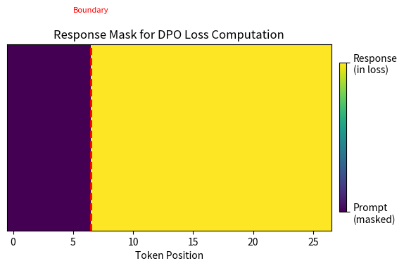
The response mask is critical: it tells us which token positions should contribute to the DPO loss. We only want to compare log probabilities over the response tokens, not the shared prompt.

With properly formatted data, we can now implement the DPO loss function. This objective encourages the model to assign higher implicit rewards to chosen responses while constraining the model to stay close to the reference policy. DPO transforms a reinforcement learning problem into a simple classification task: given a pair of responses, predict which one humans would prefer. Recall from the DPO Derivation chapter that the loss is defined as:

where:

• $\pi_\theta$: the policy model being trained
• $\pi_\text{ref}$: the frozen reference model (usually the initial version of $\pi_\theta$)
• $\mathcal{D}$: the dataset of preference triplets $(x, y_w, y_l)$
• $\mathbb{E}_{(x, y_w, y_l) \sim \mathcal{D}}$: the expected value over preference triplets drawn from the dataset (computed as a batch average)
• $x$: the prompt or instruction
• $y_w$: the chosen (winning) response
• $y_l$: the rejected (losing) response
• $\beta$: a temperature parameter scaling the strength of the preference constraint
• $\sigma$: the logistic sigmoid function, $\sigma(z) = \frac{1}{1 + e^{-z}}$

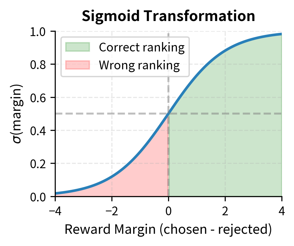
To understand this formula intuitively, consider what each component accomplishes. The log ratio $\log \frac{\pi_\theta(y|x)}{\pi_\text{ref}(y|x)}$ measures how much more (or less) likely the policy model finds a response compared to the reference model. When this ratio is positive, the policy has increased its probability for that response relative to where it started. When negative, the policy has decreased its probability. The term $\beta \log \frac{\pi_\theta(y|x)}{\pi_\text{ref}(y|x)}$ represents the implicit reward the model assigns to a response, capturing the idea that preferred responses should see increased probability while rejected responses should see decreased probability.

The difference between these implicit rewards for the chosen and rejected responses measures how well the model has learned the preference. If this difference is large and positive, the model strongly prefers the chosen response. The sigmoid function $\sigma$ converts this difference into a probability, and by taking the negative log, we arrive at a cross-entropy loss that pushes the model to make this probability as high as possible.

By minimizing this negative log-likelihood, DPO optimizes the policy so that the implicit reward for the chosen response $y_w$ is higher than for the rejected response $y_l$. DPO steers the model toward human preferences while staying close to the reference policy using only supervised learning.

First, compute the log probability $\log \pi(y|x)$ for a response $y$ given prompt $x$. This computation is the foundation of the DPO loss. Since autoregressive models generate text one token at a time, each token's probability depends on all previous tokens. We calculate the total sequence probability by summing the log probabilities of each token conditioned on its history:

where:

• $y$: the full response sequence
• $x$: the input prompt
• $|y|$: the total number of tokens in the response
• $y_t$: the token at position $t$
• $y_{<t}$: the sequence of tokens preceding $t$ (the history)
• $\sum_{t=1}^{|y|}$: the sum of log probabilities across all tokens in the sequence

This formula arises from the chain rule of probability. The probability of generating an entire sequence equals the product of generating each token given everything that came before it. In log space, the product of token probabilities becomes a sum, which is numerically stable and computationally convenient. Each term $\log \pi(y_t | x, y_{<t})$ represents the model's confidence in predicting token $y_t$ given the prompt $x$ and all previously generated tokens $y_{<t}$.

This summation computes the total log probability of the sequence by aggregating the log probabilities of each token conditioned on its history. Longer sequences have lower log probabilities because they contain more terms. Comparing log ratios rather than raw log probabilities cancels out length effects when comparing the same response under different models.

This function handles the critical shift operation for next-token prediction: since logits at position $t$ predict token at position $t+1$, we need to align everything properly. This alignment is a common source of bugs in language model implementations, so it deserves careful attention. The model's output at each position represents a probability distribution over what the next token should be, not what the current token is. Therefore, to find the probability assigned to each actual token in the sequence, we must look at the logits from the preceding position.

Now we can implement the full DPO loss. This function brings together all the components we've discussed: computing log probabilities for both the policy and reference models on both chosen and rejected responses, calculating the log ratios that represent implicit rewards, and combining them through the sigmoid to produce a differentiable loss signal.

These metrics help monitor training:

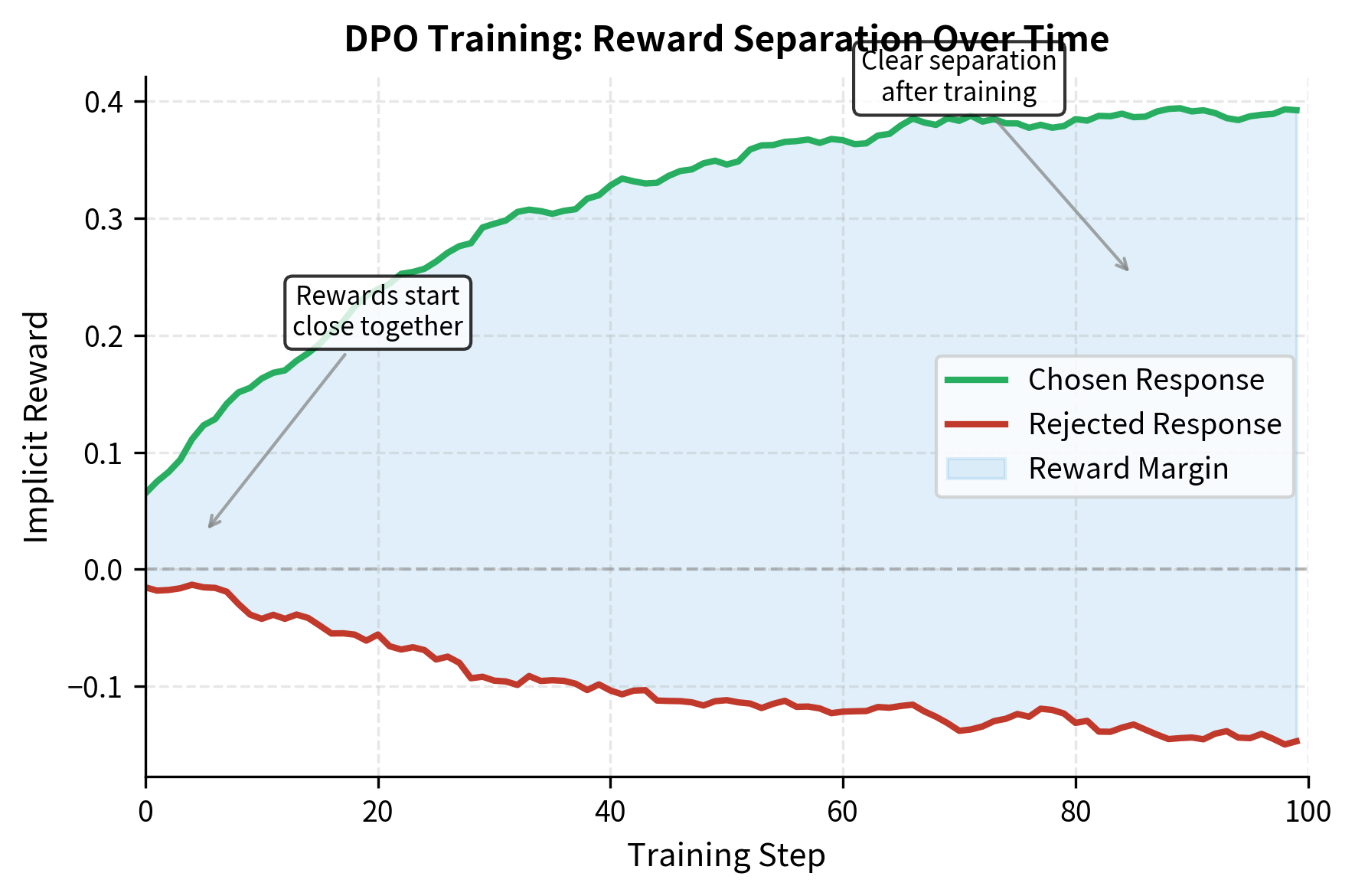
• Reward margin: The average difference between implicit rewards for chosen and rejected responses. This should increase during training as the model learns to more strongly prefer the chosen responses. A growing reward margin indicates the model is successfully learning the preference signal.
• Accuracy: The fraction of examples where the policy assigns higher implicit reward to the chosen response. Well-trained models should approach high accuracy on the training set. However, reaching 100% accuracy too quickly or too easily may indicate overfitting.
• Individual rewards: Tracking both chosen and rejected rewards helps diagnose issues like reward hacking. Ideally, the chosen reward should increase modestly while the rejected reward decreases or stays stable. If both rewards increase dramatically, the model may be drifting too far from the reference policy.

The DPO loss involves log probabilities that can become very negative for long sequences. A sequence of 100 tokens where each token has an average log probability of -3 would yield a sequence log probability of -300. While this doesn't cause issues when computing ratios, the computation remains stable for several reasons.

A few practices help maintain numerical stability:

Working with log ratios rather than raw probabilities ensures numerical stability. When we compute $\log \pi_\theta(y|x) - \log \pi_\text{ref}(y|x)$, the very negative values from long sequences largely cancel out, leaving a ratio that reflects how differently the two models view the same response. This cancellation is what keeps the numbers in a manageable range.

Label smoothing can be helpful when your preference labels are noisy, as discussed in the Human Preference Data chapter. Setting a small smoothing value (0.01-0.1) prevents the model from becoming overconfident about potentially mislabeled examples. The smoothing works by mixing in a small probability of the "wrong" label, which acts as a form of regularization that improves generalization when the training data contains annotation errors.

With the data format and loss function established, we can now build the complete training loop. DPO training has several unique aspects compared to standard fine-tuning.

The reference model $\pi_\text{ref}$ must remain frozen throughout training. There are two common approaches:

Approach 1: Separate Model Copy

Load two copies of the model, freezing one:

This approach is simple but doubles memory usage. For large models, this may be prohibitive.

Approach 2: LoRA with Shared Base

When using LoRA (covered in Part XXV), the reference model is implicitly the base model with LoRA adapters disabled:

With LoRA, you compute reference log probabilities by temporarily disabling the adapters using model.disable_adapter_layers().

Here's a complete training implementation:

Let's train on our small demonstration dataset:

We successfully loaded a small GPT-2 model with approximately 124 million parameters and prepared a dataloader with 2 batches. This setup allows for quick iteration during this demonstration.

The training completes successfully, showing a decrease in loss and an increase in accuracy and reward margin. This indicates the policy model is learning to assign higher implicit rewards to the chosen responses compared to the rejected ones.

Monitoring the right metrics helps diagnose training issues:

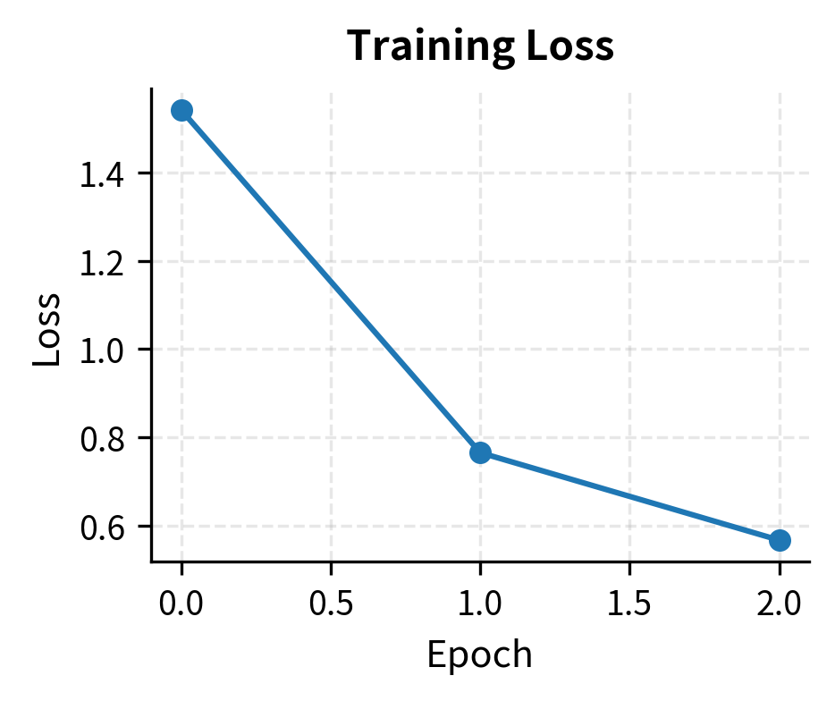
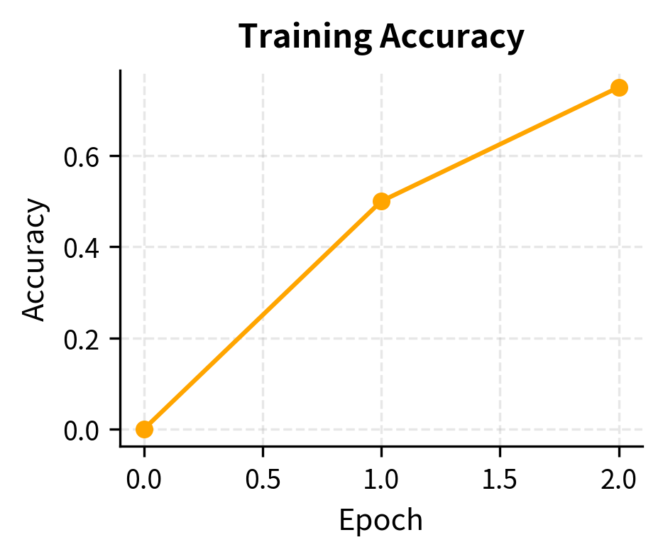
The plots show two complementary trends: the training loss consistently decreases, indicating the model is minimizing the DPO objective, while the ranking accuracy improves, confirming that the model increasingly prefers the chosen responses over the rejected ones.

DPO has fewer hyperparameters than RLHF, but choosing them well is crucial for successful training.

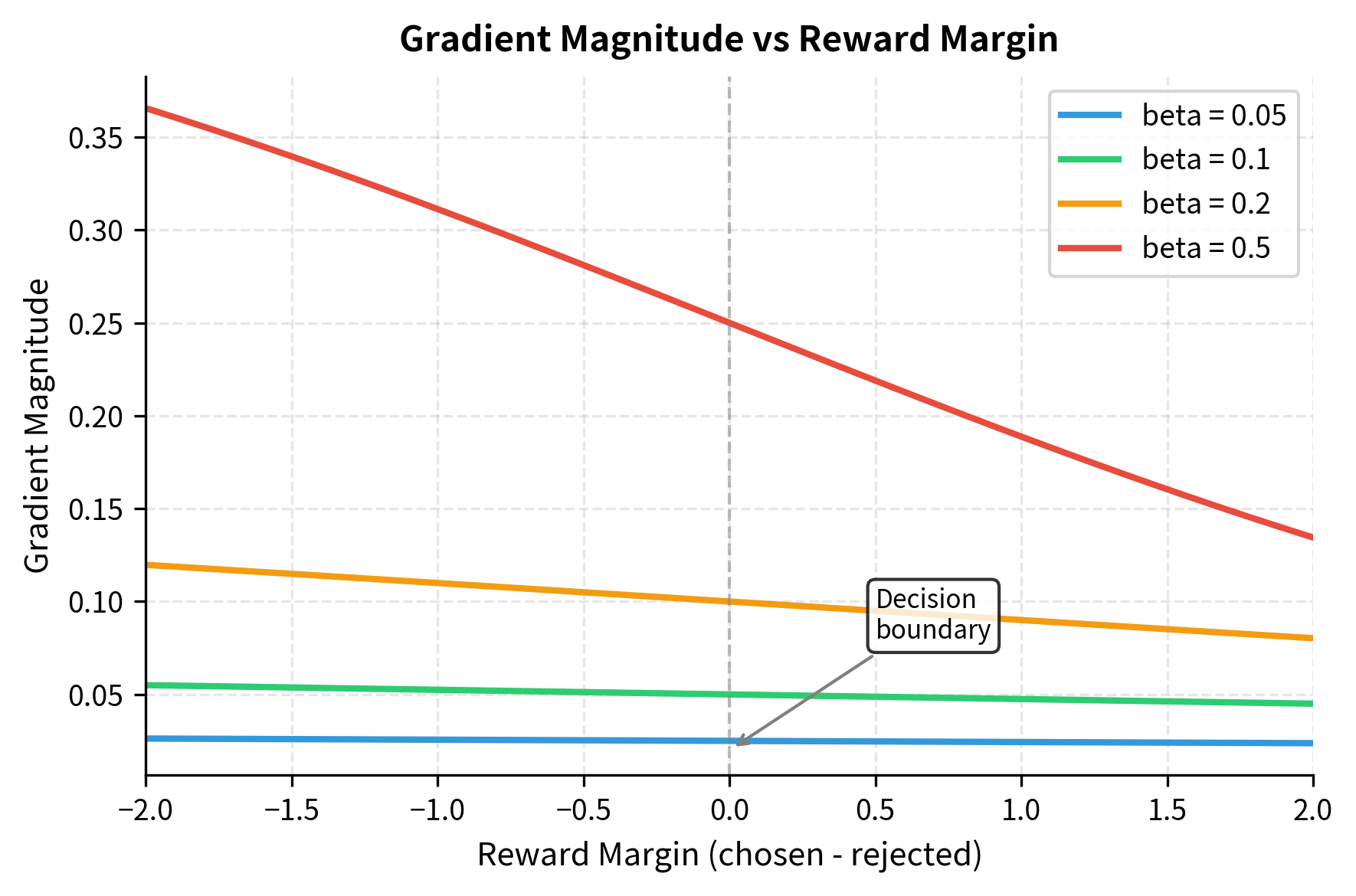
The $\beta$ parameter is the most important hyperparameter in DPO. It controls the strength of the KL divergence constraint between the policy and reference model. The implicit reward for a response is $\beta \log \frac{\pi_\theta(y|x)}{\pi_\text{ref}(y|x)}$. The $\beta$ parameter scales this entire quantity, effectively determining how much the model is "allowed" to deviate from the reference policy.

Low $\beta$ (0.01-0.1):

• Allows larger deviations from the reference policy
• Faster learning but higher risk of overfitting to preference data
• May lead to degenerate outputs or reward hacking

When $\beta$ is small, the implicit reward signal is weak, meaning the model must make large probability changes to achieve a significant reward difference. This encourages aggressive updates that can quickly overfit to the training data.

High $\beta$ (0.5-1.0):

• Strong regularization toward the reference model
• More conservative updates, slower learning
• Better preservation of general capabilities but may underfit preferences

When $\beta$ is large, even small deviations from the reference policy produce large implicit rewards or penalties. This makes the model cautious about straying too far from its initial behavior.

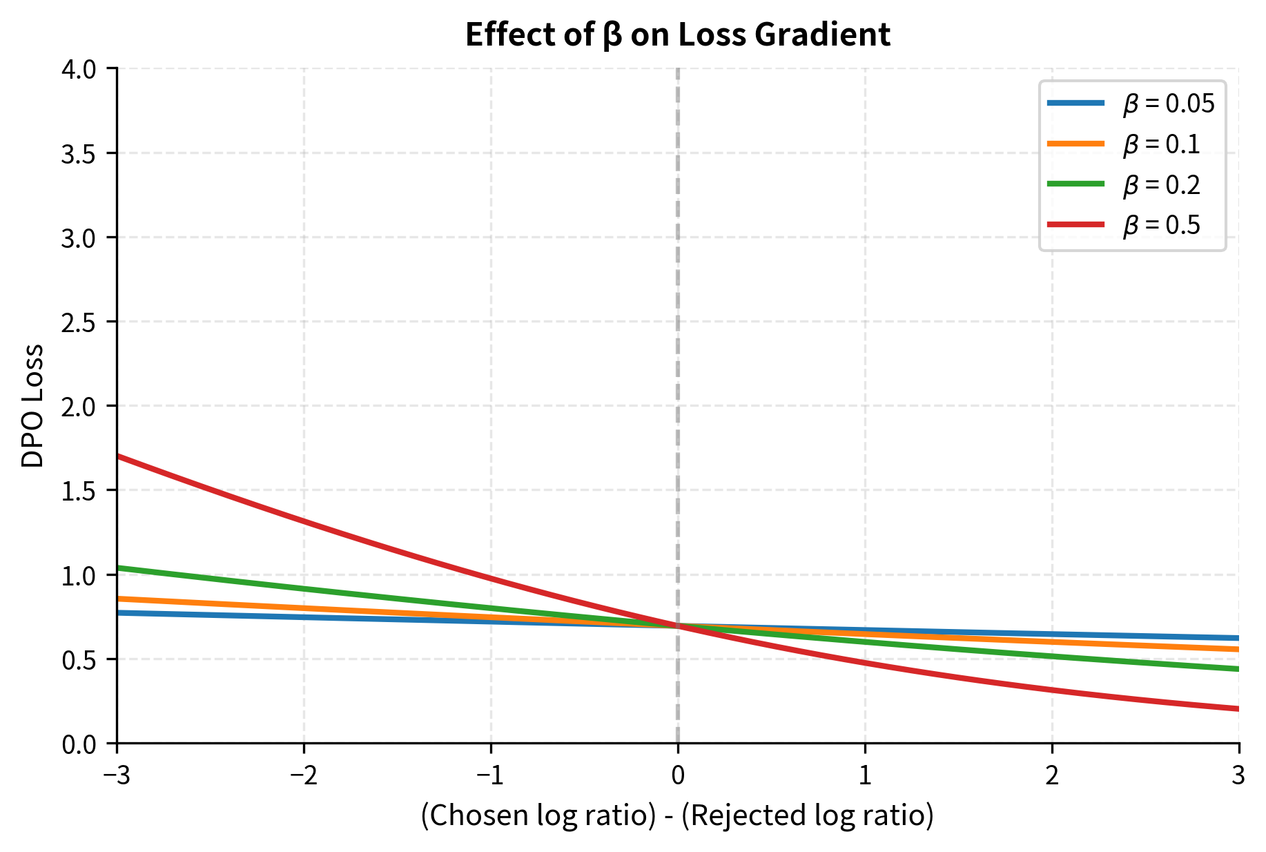
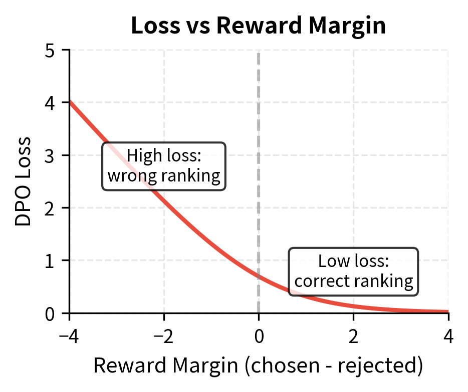
The original DPO paper found $\beta = 0.1$ to work well across a variety of tasks. This value provides a reasonable balance between learning preferences and maintaining coherence. The visualization reveals why: at $\beta = 0.1$, the loss curve has a moderate slope that provides clear gradient signal without being so steep that small changes in log ratios cause dramatic loss changes.

DPO typically requires smaller learning rates than supervised fine-tuning:

• Full fine-tuning: 1e-6 to 5e-6
• LoRA fine-tuning: 1e-5 to 5e-5

The smaller rates are necessary because DPO directly optimizes log probability ratios, which can change rapidly with small weight updates. Unlike supervised fine-tuning where we're simply maximizing the likelihood of target tokens, DPO computes a ratio between two model evaluations. Small changes to the policy model affect both the numerator and denominator of this ratio, potentially causing the implicit reward to shift dramatically if the learning rate is too high.

These guidelines provide a starting point for tuning. The learning rate is particularly critical; starting too high often destabilizes the implicit reward formulation, leading to poor convergence.

DPO benefits from larger effective batch sizes because the loss depends on comparing policy and reference log probability ratios. Small batches introduce variance in these estimates, which can make training noisy and unstable. With a larger batch, the average over multiple preference pairs provides a more reliable gradient signal.

If GPU memory is limited, use gradient accumulation:

DPO typically converges faster than you might expect. One to three epochs over the preference data is usually sufficient. Overfitting is a real concern: if accuracy reaches 100% on training data but generations become repetitive or degenerate, you've overfit.

Signs of overfitting include:

• Training accuracy approaches 100% while validation loss increases
• Generated text becomes repetitive or templated
• The model loses diversity in its responses

Production DPO training requires additional considerations.

For large models, computing forward passes for both policy and reference models strains memory. The TRL library from Hugging Face provides optimized implementations:

Beyond loss and accuracy, monitor generation quality:

Periodically generating responses to held-out prompts and reviewing them manually (or with an LLM judge) provides crucial signal about whether DPO is achieving its intended effect.

DPO has made preference-based alignment more accessible by eliminating the complexity of reward model training and reinforcement learning. However, implementation challenges remain.

DPO is only as good as your preference data. Unlike RLHF where a reward model can generalize learned preferences to new situations, DPO directly optimizes for the specific comparisons in your training set. This means noisy labels, biased annotators, or unrepresentative prompt distributions will directly impact the aligned model.

In practice, data curation often matters more than algorithmic improvements. Teams investing in DPO should allocate significant effort to preference data quality: establishing clear annotation guidelines, measuring inter-annotator agreement, and filtering low-confidence examples.

With very small $\beta$ values or prolonged training, DPO can collapse toward generating only responses very similar to the "chosen" examples in the training data. This manifests as reduced response diversity and over-fitting to surface patterns in preferred responses rather than learning the underlying preference criteria.

Monitoring response diversity during training and using techniques like early stopping or label smoothing can mitigate this risk. Some practitioners also mix DPO training with continued language modeling loss to maintain general capabilities.

As models grow larger, the memory requirements for maintaining both policy and reference models become significant. Even with LoRA, computing forward passes through large models twice (once with adapters, once without) adds computational overhead. The DPO Variants chapter covers techniques like reference-free DPO that address some of these challenges.

Despite these limitations, DPO has become the preferred alignment method for many teams due to its simplicity and effectiveness. Aligning models with preference data using supervised learning infrastructure makes alignment research more accessible.

The key parameters for DPO training are:

• beta: Controls the strength of the KL divergence constraint (typically 0.1). Higher values keep the policy closer to the reference model.
• learning_rate: The step size for optimization (typically 5e-7 to 1e-5). DPO requires lower rates than standard supervised fine-tuning.
• batch_size: The number of samples processed per step. Larger batches generally stabilize the loss estimate.

This chapter translated DPO theory into practice. The key implementation components are:

Data format: DPO requires triplets of (prompt, chosen response, rejected response), with careful tokenization to identify which tokens belong to the response versus the prompt.

Loss computation: The DPO loss compares log probability ratios between the policy and reference model for chosen versus rejected responses. Proper handling of sequence masking and numerical stability is essential.

Training procedure: DPO training requires maintaining a frozen reference model (either as a separate copy or implicitly through LoRA). Standard supervised learning infrastructure handles the rest.

Hyperparameters: The $\beta$ parameter controls the KL constraint strength, with typical values around 0.1. Learning rates should be lower than standard fine-tuning, and DPO often converges in just one to three epochs.

With these components in place, you can align language models to human preferences without the complexity of reward modeling and reinforcement learning that RLHF requires. The next chapter explores variants of DPO that address specific limitations, including methods that eliminate the need for a reference model entirely.

Ready to test your understanding? Take this quick quiz to reinforce what you've learned about DPO implementation.