

Derive the DPO loss function from first principles. Learn how the optimal RLHF policy leads to reward reparameterization and direct preference optimization.

This article is part of the free-to-read Language AI Handbook
Choose your expertise level to adjust how many terms are explained. Beginners see more tooltips, experts see fewer to maintain reading flow. Hover over underlined terms for instant definitions.
DPO Derivation
In the previous chapter, we introduced Direct Preference Optimization as a simpler alternative to RLHF that eliminates the need for an explicit reward model. We saw that DPO directly optimizes a language model using preference data, but we didn't examine why this works or how the DPO loss function is derived. This chapter fills that gap.
The DPO derivation is a key result in alignment research. It shows that the optimal policy for the RLHF objective has a closed-form solution, and this solution can be rearranged to express the implicit reward in terms of the policy itself. When we substitute this reparameterized reward into the Bradley-Terry preference model, we obtain the DPO loss function directly, with no reinforcement learning required.
Understanding this derivation reveals why DPO works, its underlying assumptions, and how to interpret the model's learning process. By the end of this chapter, you'll see that DPO is essentially solving a classification problem where the model learns to assign higher probability to preferred responses.
The RLHF Objective
Let's begin with the objective that RLHF aims to optimize. As we discussed in the chapters on PPO for Language Models and KL Divergence Penalty, the goal is to find a policy that maximizes expected reward while staying close to a reference policy (typically the supervised fine-tuned model).
Before diving into the mathematics, it helps to understand the intuition behind this objective. We want our language model to generate responses that humans prefer, which is captured by the reward function. However, if we optimize the reward too aggressively, the model might find unexpected shortcuts or produce degenerate outputs that technically achieve high reward but don't represent genuinely helpful behavior. The reference policy serves as an anchor, representing the model's pre-trained knowledge and natural language capabilities. By penalizing deviations from this anchor, we encourage the model to improve its outputs while maintaining coherent, fluent generation.
The constrained optimization problem is:
where:
- : the policy being optimized
- : the expectation operator
- : a prompt sampled from the data distribution
- : a response sampled from the policy
- : the learned reward function
- : a hyperparameter controlling the strength of the KL constraint
- : the Kullback-Leibler divergence
- : the reference policy
To work with this objective more directly, we need to expand the KL divergence term. Recall that the KL divergence measures how different one probability distribution is from another, expressed as the expected log ratio of the two distributions. Writing out the KL divergence explicitly, this becomes:
where:
- : the expectation operator
- : the data distribution
- : the reward function
- : the KL penalty coefficient
- : the natural logarithm
- : probability of response given prompt under the policy
- : probability of response given prompt under the reference model
This reformulation reveals the objective's structure more clearly. The log ratio measures how much the policy has shifted away from the reference for a particular response. When this ratio is positive (the policy assigns more probability than the reference), the KL term subtracts from the objective, penalizing the deviation. When the ratio is negative (the policy assigns less probability), the term adds to the objective, which might seem like a reward, but since we're sampling from , we're unlikely to generate responses where assigns low probability.
This objective captures a fundamental tension in alignment: we want the model to produce high-reward outputs (as judged by human preferences), but we don't want it to deviate too far from its pre-trained behavior. Without the KL penalty, the model might find degenerate solutions that exploit flaws in the reward model, a phenomenon we explored in the chapter on Reward Hacking.
Deriving the Optimal Policy
The key insight behind DPO is that this optimization problem has a closed-form solution. Unlike many optimization problems in machine learning that require iterative gradient descent, this particular formulation admits an analytical answer. For a fixed prompt , we're optimizing over the distribution for all possible responses . This is a constrained optimization problem over probability distributions: we must ensure our solution is a valid probability distribution that sums to one and assigns non-negative probability to every possible response.
The special structure of the RLHF objective allows for this closed-form solution. The expectation under combined with the KL divergence creates what's known as a variational problem over distributions. Such problems often have elegant solutions when the constraints are simple probability simplex constraints.
Let's work through the derivation step by step. For a single prompt , the objective is:
where:
- : sum over all possible responses in the vocabulary
- : the entire probability distribution over responses for prompt
- : probability of response given prompt
- : the reward function
- : the KL penalty coefficient
- : the natural logarithm
- : the reference policy probability
We need to maximize this subject to the constraint that is a valid probability distribution: and for all .
To solve this constrained optimization problem, we use the method of Lagrange multipliers, a classical technique from calculus. The idea is to incorporate the constraint directly into the objective by introducing a new variable (the Lagrange multiplier) that penalizes violations of the constraint. At the optimal solution, the gradient of the objective with respect to the decision variables must be proportional to the gradient of the constraint.
The Lagrangian is:
where:
- : the Lagrangian function
- : sum over all responses
- : probability of response
- : the reward function
- : the KL penalty coefficient
- : the natural logarithm
- : the reference policy probability
- : the Lagrange multiplier for the constraint that probabilities sum to 1
Notice that we've expanded the log ratio term from the original objective, separating it into and . This separation makes taking derivatives more straightforward. The term enforces our normalization constraint: if the probabilities don't sum to one, this term will be nonzero, and the Lagrange multiplier will adjust to push us toward a valid distribution.
Taking the derivative with respect to for a specific :
where:
- : the partial derivative of the Lagrangian with respect to the probability of response
- : the reward function
- : the KL penalty coefficient
- : the natural logarithm
- : the policy probability
- : the reference policy probability
- : the Lagrange multiplier
The term comes from differentiating , which gives . This is a standard result from calculus: when we differentiate with respect to , we apply the product rule, obtaining . Setting this derivative equal to zero gives us the first-order optimality conditions.
Solving for :
where:
- : the log-probability of response
- : the reward function
- : the KL penalty coefficient
- : the reference policy probability
- : constant terms related to the normalization constraint
This expression for the log-probability has an illuminating structure. The log-probability under our optimal policy equals the log-probability under the reference, adjusted by the scaled reward , plus some constants that don't depend on . Higher reward responses get higher log-probabilities, with controlling how much the reward matters relative to staying close to the reference.
Exponentiating both sides:
where:
- : the policy probability
- : the reference policy probability
- : the exponential function
- : the reward-scaling term
- : the reward function
- : the KL penalty coefficient
- : the normalization term constant across all
The term is just a normalizing constant that ensures the distribution sums to 1. Crucially, this term doesn't depend on ; it only depends on through the constraint that all probabilities must sum to one. We can absorb it into a partition function :
where:
- : the optimal policy distribution
- : the partition function (normalizing constant) for prompt
- : the reference policy distribution
- : the reward function
- : the temperature parameter
This is the optimal policy for the RLHF objective. It has a clear interpretation: the optimal policy takes the reference distribution and reweights each response by the exponentiated reward, then normalizes. The exponential function ensures all probabilities are positive, naturally satisfying the constraint. Responses with higher reward get exponentially more probability mass, with controlling how aggressively we reweight.
Consider what happens at extreme values of beta to see how this reweighting works. When is very large, the reward term becomes small, and for all responses. In this limit, the optimal policy stays very close to the reference distribution, barely adjusting for reward at all. Conversely, when is very small, the exponential amplifies small reward differences into massive probability shifts, concentrating all probability mass on the highest-reward response. The choice of therefore controls the exploration-exploitation trade-off: larger values favor staying close to the reference (exploration), while smaller values favor chasing high reward (exploitation).
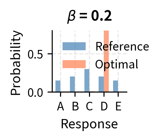
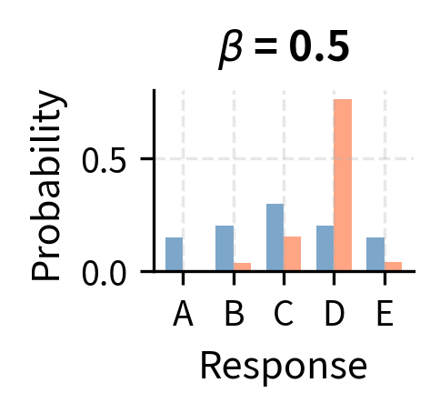
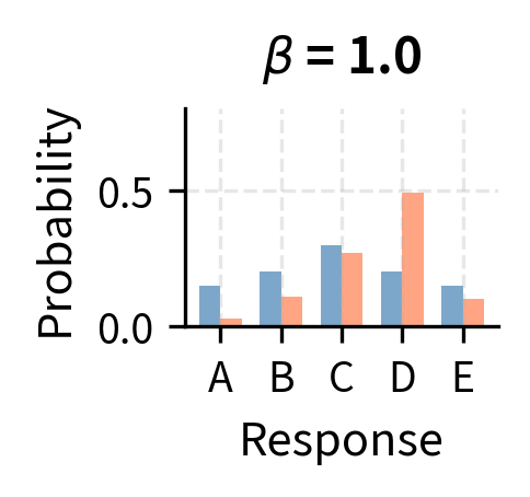
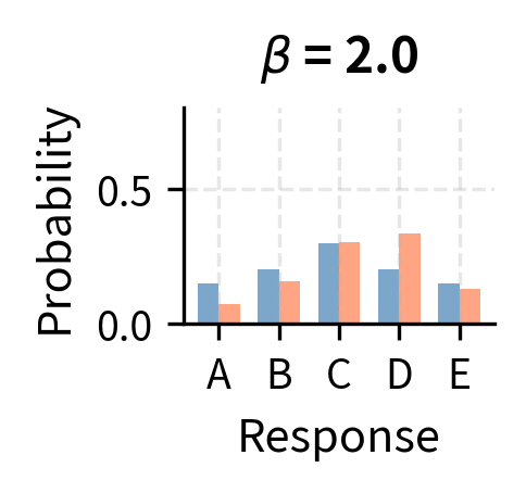
The optimal policy has the form of a Boltzmann (or Gibbs) distribution from statistical mechanics, where plays the role of negative energy and plays the role of temperature. Lower temperature (smaller ) concentrates probability on the highest-reward responses.
Reparameterizing the Reward
Here's where the DPO derivation becomes clever. We've derived that the optimal policy has a specific relationship to the reward function. But we can also go backwards: given an optimal policy, we can solve for what reward function it implies.
This reverse direction might seem like a mathematical curiosity, but it turns out to be the key insight that makes DPO possible. If we can express the reward purely in terms of policies (without needing to train a separate reward model), then we can substitute this expression into the preference model and optimize directly. The reward becomes implicit in the policy rather than explicit in a separate neural network.
Starting from:
where:
- : the optimal policy distribution
- : the partition function
- : the reference policy distribution
- : the reward function
- : the temperature parameter
We can rearrange to isolate the reward. First, take the log of both sides:
where:
- : log-probability under the optimal policy
- : log-probability under the reference policy
- : the reward function
- : the KL penalty coefficient
- : log of the partition function (depends only on )
Taking the logarithm transforms our multiplicative relationship into an additive one, making algebraic manipulation simpler. The logarithm of a product becomes a sum of logarithms, and the logarithm of the exponential simply returns its argument.
Now, we rearrange terms to solve for :
where:
- : the implicit reward
- : the KL penalty coefficient
- : the optimal policy
- : the reference policy
- : the partition function
- : the scaled log-ratio term
This is the reward reparameterization. It tells us that for any optimal policy , we can express the implicit reward purely in terms of log probability ratios, plus a prompt-dependent constant .
The log ratio has a natural interpretation: it measures how much the optimal policy has increased or decreased the probability of response compared to the reference. Responses that the optimal policy strongly prefers will have large positive log ratios, while responses it disfavors will have large negative log ratios. This log ratio, scaled by , gives us the implicit reward up to an additive constant.
The partition function doesn't depend on ; it only depends on the prompt . This will turn out to be crucial because when we compute preference probabilities, this term cancels out.
The DPO Loss Function
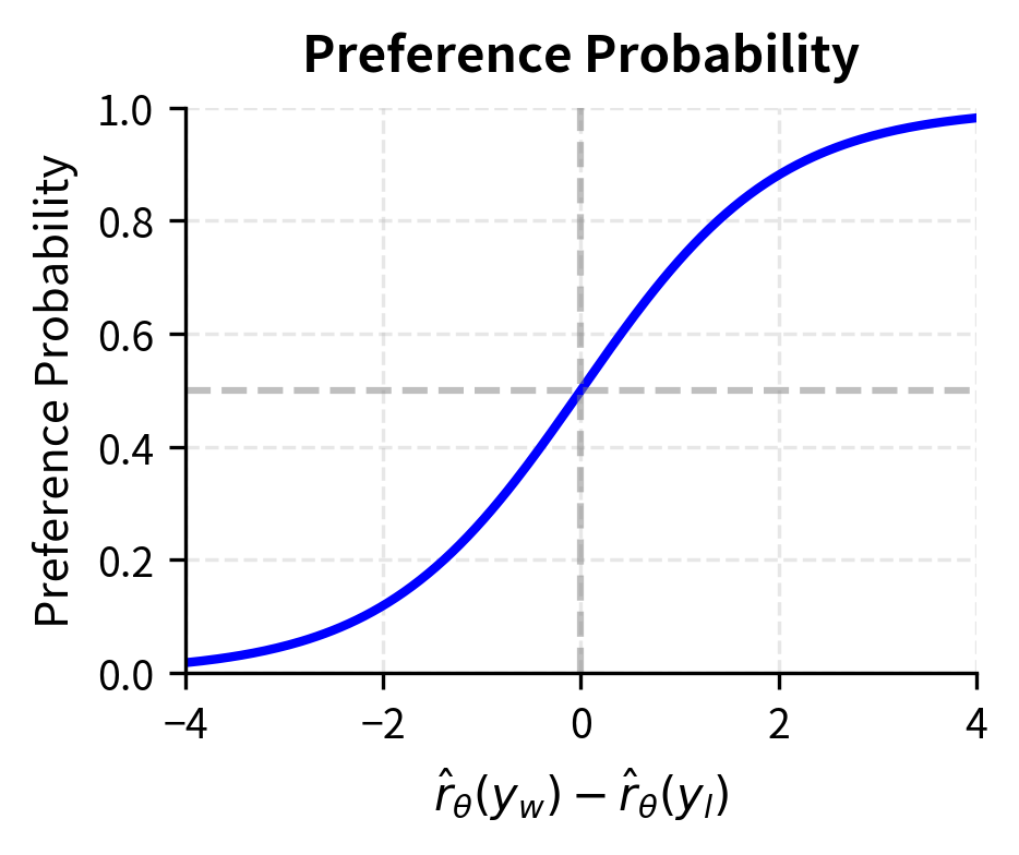
Now we can derive the DPO loss by substituting our reward reparameterization into the Bradley-Terry preference model. Recall from the chapter on the Bradley-Terry Model that the probability of preferring response over response is:
where:
- : probability that response is preferred over
- : the sigmoid function mapping values to
- : reward for the winning response
- : reward for the losing response
The Bradley-Terry model is elegant in its simplicity: the probability of preferring one response over another depends only on the difference in their rewards, passed through a sigmoid function. This means responses with much higher reward are strongly preferred, while responses with similar rewards have preference probabilities close to 0.5.
Substituting our reparameterized reward:
where:
- : the sigmoid function
- : the temperature parameter
- : the optimal policy
- : the reference policy
- : the partition function terms which appear with opposite signs
Notice that the terms cancel! This cancellation is not a coincidence; it's a direct consequence of using reward differences in the Bradley-Terry model. The partition function contributes equally to both rewards, so when we subtract them, it disappears. This cancellation is essential for the practical success of DPO because computing would require summing over all possible responses, which is computationally intractable for language models with exponentially large output spaces.
This leaves:
where:
- : the sigmoid function
- : temperature parameter
- : the optimal policy
- : the reference policy
We can simplify this using logarithm properties:
where:
- : the sigmoid function
- : the KL penalty coefficient
- : the log-likelihood ratio of the optimal policy vs reference
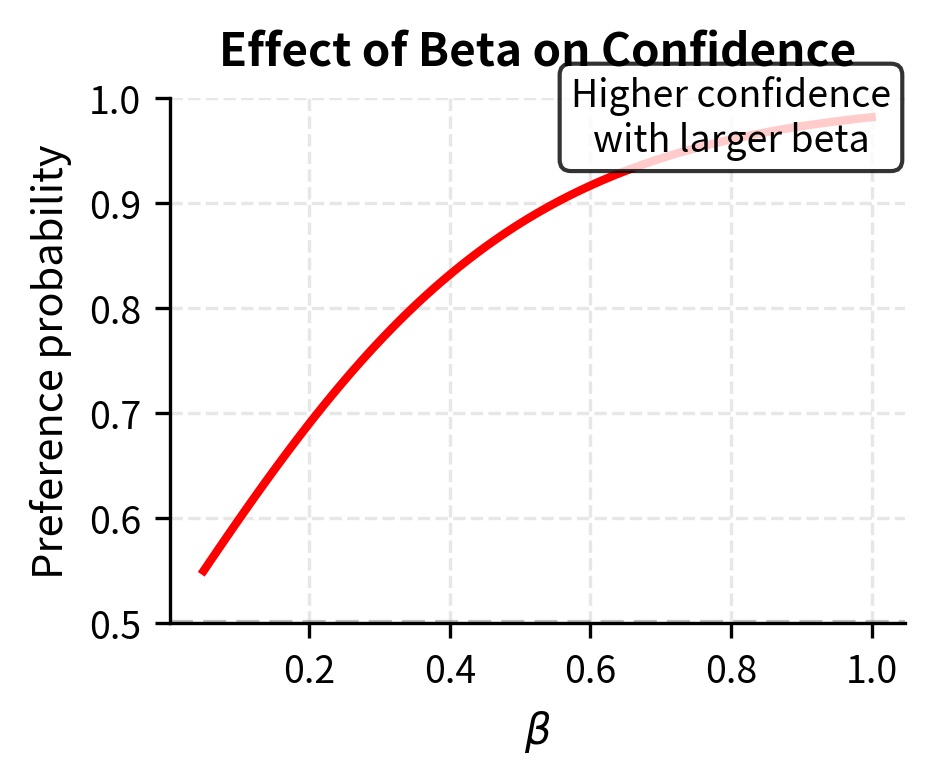
This expression is remarkably clean. The probability of the correct preference depends entirely on the difference between two log ratios: how much the optimal policy prefers the winning response (relative to the reference) versus how much it prefers the losing response. When this difference is large and positive, the sigmoid outputs a value close to 1, indicating strong confidence in the correct preference.
This is the probability that the optimal policy assigns to the correct preference. To train a policy to match this optimal policy, we maximize the log-likelihood of the observed preferences:
where:
- : the DPO loss function
- : the policy network being trained (parameterized by )
- : the reference policy
- : the dataset of preference pairs
- : expectation over the dataset
- : the KL penalty coefficient
- : the sigmoid function
The negative sign appears because we're minimizing a loss rather than maximizing likelihood.
To make the notation more compact, define the log-ratio for a response :
where:
- : the implicit reward assigned by the current model
- : the KL penalty coefficient scaling the reward
- : the policy probability
- : the reference policy probability
- : the log-ratio of the policy probability to the reference probability
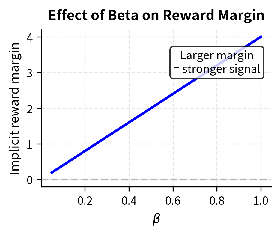
This is sometimes called the "implicit reward" because it's what the reward would be if were optimal. The terminology is fitting: we never explicitly compute or learn a reward function, yet the policy implicitly defines one through its log-probability ratios with the reference model.
The DPO loss becomes:
where:
- : the DPO loss function
- : the implicit reward function
- : the margin between implicit rewards for winning and losing responses
- : the sigmoid function
- : expectation over the dataset
This is remarkably simple. The loss encourages the model to increase its log probability (relative to the reference) on preferred responses and decrease it on dispreferred responses.
DPO as Classification
The DPO loss has a revealing interpretation: it's essentially binary classification with a specific parameterization. Consider a standard binary cross-entropy loss for classifying which of two responses is preferred:
where:
- : Binary Cross-Entropy loss
- : a scoring function indicating preference strength
- : the sigmoid function
- : expectation over the dataset
In this context, is some function that should output a positive value when is truly preferred. In DPO, this function is:
where:
- : the logit fed into the sigmoid classifier
- : the KL penalty coefficient
- : the policy network
- : the reference policy
The model is learning to classify preference pairs by adjusting its output probabilities. When the loss is low, the model assigns higher relative probability to the preferred response.
This classification view explains why DPO is so stable compared to RLHF. Instead of learning a separate reward model and then using policy gradients with their high variance, DPO directly optimizes the likelihood of preference labels. The gradients flow directly through the model's log probabilities, just like in standard language model training.
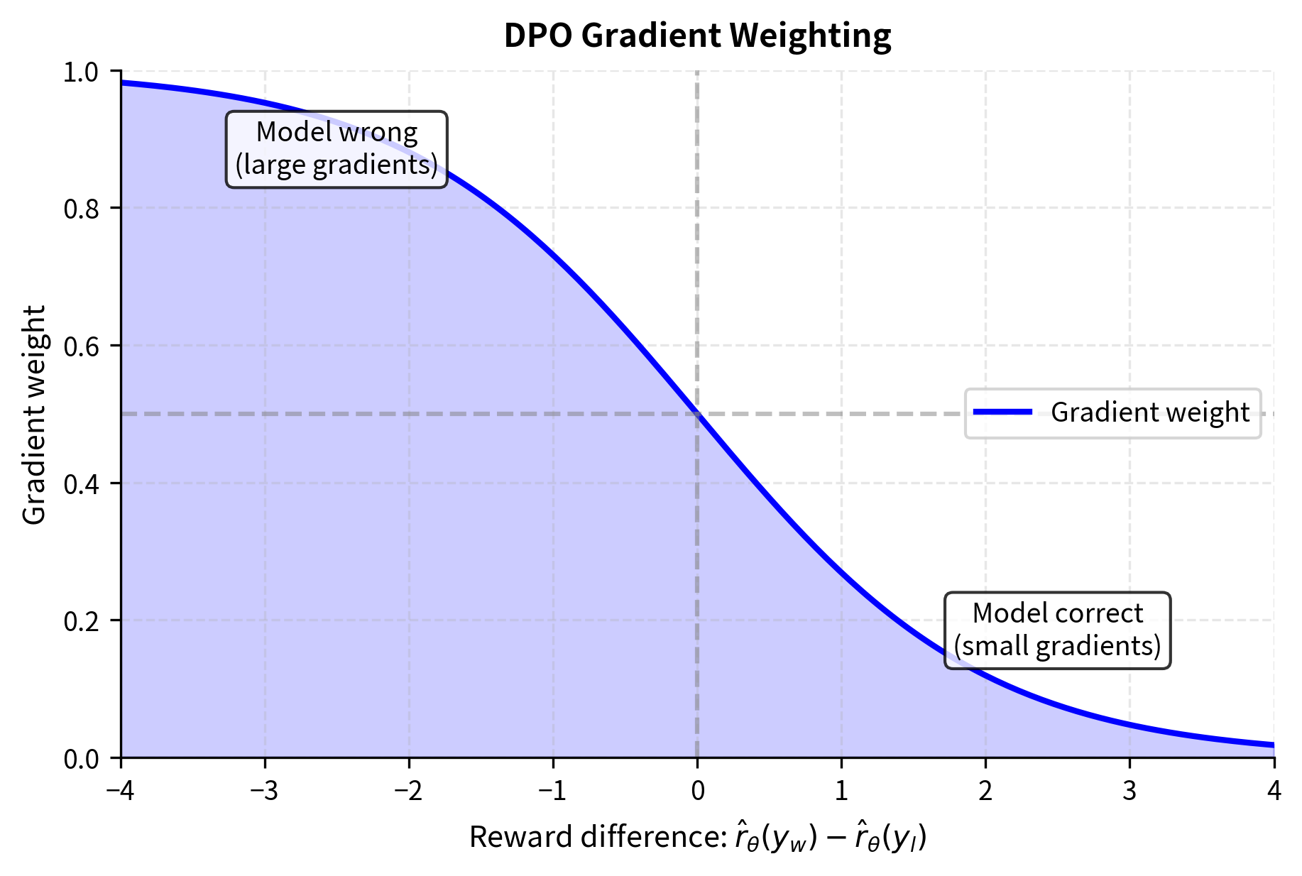
The gradient of the DPO loss with respect to has a particularly intuitive form. For a single example:
where:
- : gradient with respect to model parameters
- : the DPO loss
- : the sigmoid function
- : the implicit reward function
- : the weighting term derived from the sigmoid derivative (probability of the wrong preference)
- : the geometric gradient direction
- : the KL penalty coefficient
This gradient expression reveals the geometry of DPO optimization. The term points in the direction that increases the probability of the winning response while decreasing the probability of the losing response. This is the natural direction to push given our objective.
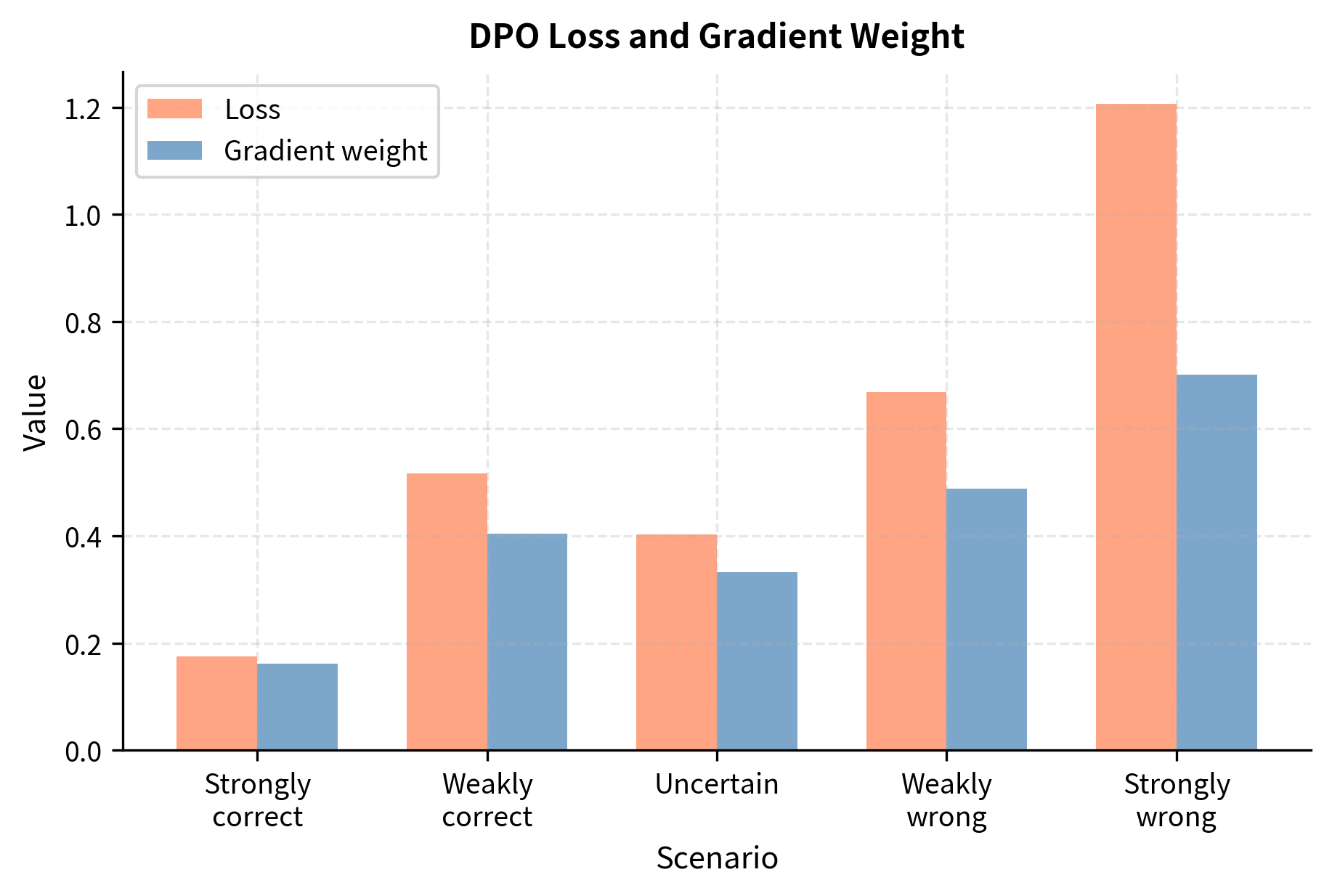
The term is the probability that the model currently assigns to the wrong preference. This acts as an implicit weighting:
- When the model is confident and correct (low wrong-preference probability), the gradient is small
- When the model is confident but wrong, the gradient is large
- When the model is uncertain, the gradient is moderate
This automatic weighting helps the model focus on examples it's getting wrong, similar to how hard negative mining works in contrastive learning.
Worked Example
Let's trace through the derivation with concrete numbers to build intuition. Suppose we have a prompt = "Write a haiku about autumn" and two responses:
- (preferred): "Crimson leaves descend / Dancing on October wind / Earth prepares to sleep"
- (dispreferred): "Leaves fall down in fall / The weather gets cold outside / I like pumpkin spice"
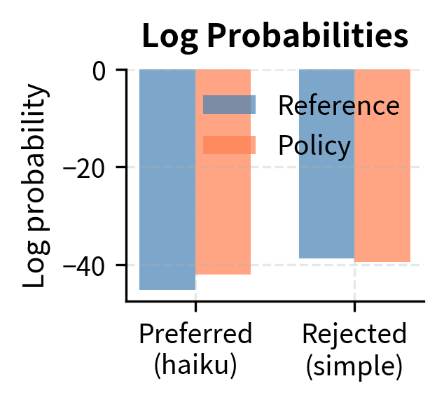
Assume our reference model assigns:
- (log probability of generating the preferred response)
- (log probability of generating the dispreferred response)
The reference model actually assigns higher probability to the dispreferred response because it's simpler and uses more common words.
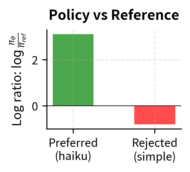
Now suppose our current policy assigns:
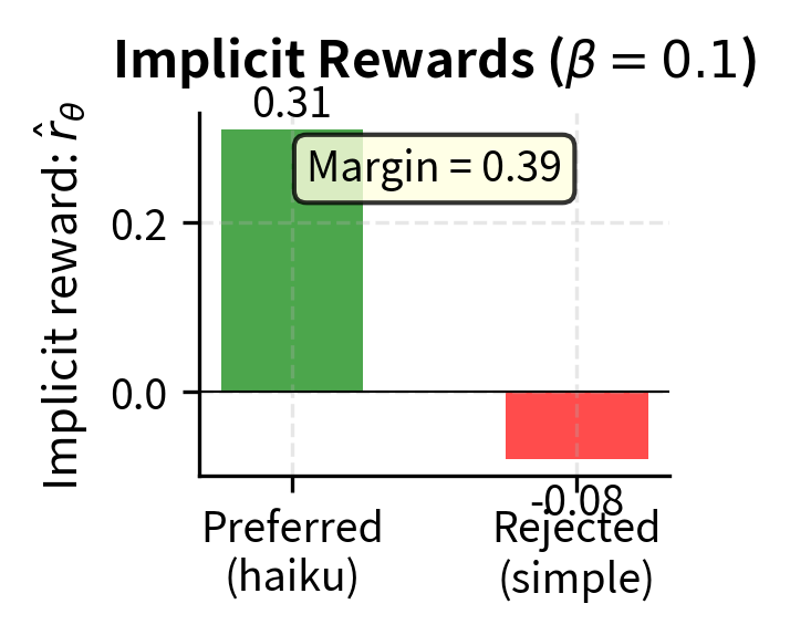
With , the implicit rewards are:
The difference is:
The loss contribution from this example:
The model is doing okay on this example (probability of correct preference is about 60%), but there's room to improve. The gradient will push the model to further increase relative to the reference and decrease relative to the reference.
Code Implementation
Let's implement the DPO loss function and verify our derivation with code.
Now let's verify with our worked example:
The implicit rewards align with our derivation: the chosen response has a positive reward (0.310), while the rejected response has a negative reward (-0.080). The positive difference (0.390) results in a preference probability of 0.596. This indicates the model correctly prefers the chosen response, though the probability is only moderately high.
Let's also visualize how the loss and preference probability change as the model learns:
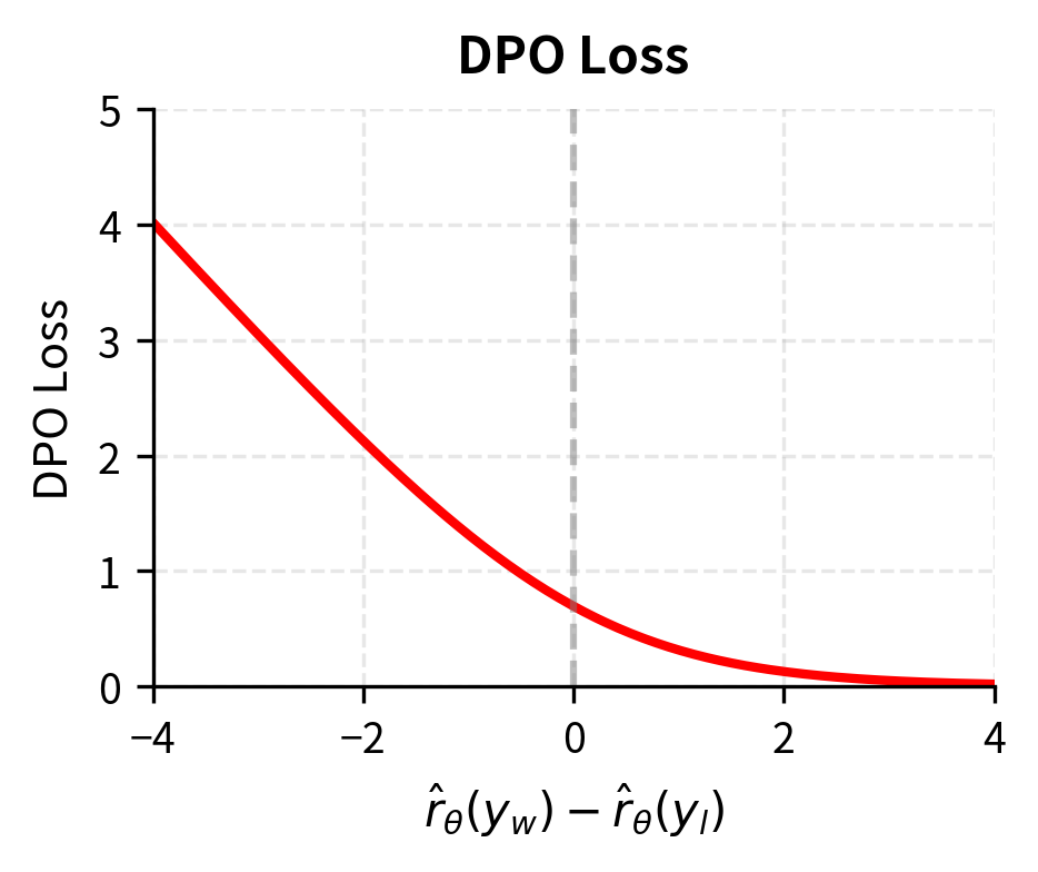
The loss approaches zero as the reward difference increases, meaning the model strongly prefers chosen responses. Conversely, when the model prefers rejected responses (negative reward difference), the loss grows large.
Let's also implement a function to compute the gradients and see how the implicit weighting works:
Notice how the gradient weight automatically adjusts based on how wrong the model is. In the "Model strongly correct" case, the gradient weight is near zero (0.000), meaning there's little to learn. Conversely, when the model is "Strongly wrong", the gradient weight approaches one (0.993), pushing hard to correct the mistake.
Key Parameters
The key parameter for DPO is:
- beta: The temperature parameter (often denoted as ) that scales the log-ratio of the policy and reference probabilities. It controls the strength of the KL divergence penalty, with larger values keeping the policy closer to the reference model.
Assumptions and Validity
The DPO derivation makes several assumptions worth examining:
-
Perfect reward model: The Bradley-Terry model with the true reward function correctly captures human preferences. In practice, human preferences are noisy, inconsistent, and context-dependent. The DPO loss treats all preference labels as ground truth, which can be problematic when labels are unreliable.
-
Boltzmann-form optimal policy: The optimal policy exists and has the Boltzmann form derived earlier. This is guaranteed for the specific RLHF objective we started with, but different formulations (such as using a different divergence measure) would yield different optimal policies and potentially different direct alignment algorithms.
-
Model capacity: DPO optimizes toward the optimal policy but doesn't guarantee reaching it. The policy is constrained by the model's architecture and capacity. A small model may not be able to represent the true optimal policy, in which case DPO finds the best approximation within the model class.
-
Reference model availability: DPO requires that we can compute exactly for the same responses we're evaluating under . This is straightforward when both are the same model architecture, but becomes complex if the reference model is unavailable or uses different tokenization. The next chapter on DPO Implementation will address these practical considerations in detail.
Summary
This chapter derived the DPO loss function from first principles, showing how it emerges naturally from the RLHF objective.
The key steps in the derivation were:
- RLHF objective: Maximize expected reward with a KL penalty to stay close to the reference policy
- Optimal policy: Using Lagrange multipliers, we found that the optimal policy is a Boltzmann distribution that reweights the reference by exponentiated rewards
- Reward reparameterization: Inverting this relationship, we expressed the implicit reward as a log-ratio between the optimal and reference policies, plus a partition function
- Bradley-Terry substitution: Plugging the reparameterized rewards into the preference model, the partition functions cancel, leaving a loss in terms of log-ratios only
- Classification view: The resulting DPO loss is binary cross-entropy, learning to classify which response is preferred based on relative log-probabilities
The gradient of the DPO loss has an automatic weighting scheme: examples where the model is confidently wrong receive larger gradients, while examples where it's already correct receive smaller gradients. This makes DPO training stable and efficient.
In the next chapter, we'll implement DPO end-to-end, covering practical details like computing sequence log-probabilities, handling padding, and integrating with Hugging Face's training infrastructure.
Quiz
Ready to test your understanding? Take this quick quiz to reinforce what you've learned about the DPO derivation.

Comments