

Learn how DPO eliminates reward models from LLM alignment. Understand the reward-policy duality that enables supervised preference learning.

This article is part of the free-to-read Language AI Handbook
Choose your expertise level to adjust how many terms are explained. Beginners see more tooltips, experts see fewer to maintain reading flow. Hover over underlined terms for instant definitions.
DPO Concept
The RLHF pipeline aligns language models with human preferences but is costly. Training requires managing three separate models (the policy, the reward model, and the reference model), running multiple forward passes during generation, and navigating the notoriously unstable dynamics of reinforcement learning. Direct Preference Optimization (DPO) asks if we can achieve alignment without the complexity of reinforcement learning. DPO reformulates the preference alignment problem as supervised learning on preference pairs, eliminating the reward model entirely while provably optimizing the same objective as RLHF. This chapter develops the conceptual foundations of DPO, building intuition for why this simplification works and examining its practical advantages. We'll save the mathematical derivation and implementation details for the following chapters. By the end of this chapter, you should understand not just what DPO does, but why it works and when you might choose it over traditional RLHF approaches.
The RLHF Complexity Problem
As we discussed in the RLHF Pipeline chapter, aligning a language model with human preferences involves a multi-stage process. First, we train a reward model on preference data, teaching a neural network to predict which responses humans prefer. Then we use that reward model to guide policy optimization through PPO, while constraining the policy to stay close to the original model via a KL divergence penalty. This pipeline, while effective, introduces several sources of complexity that create both engineering challenges and potential failure modes.
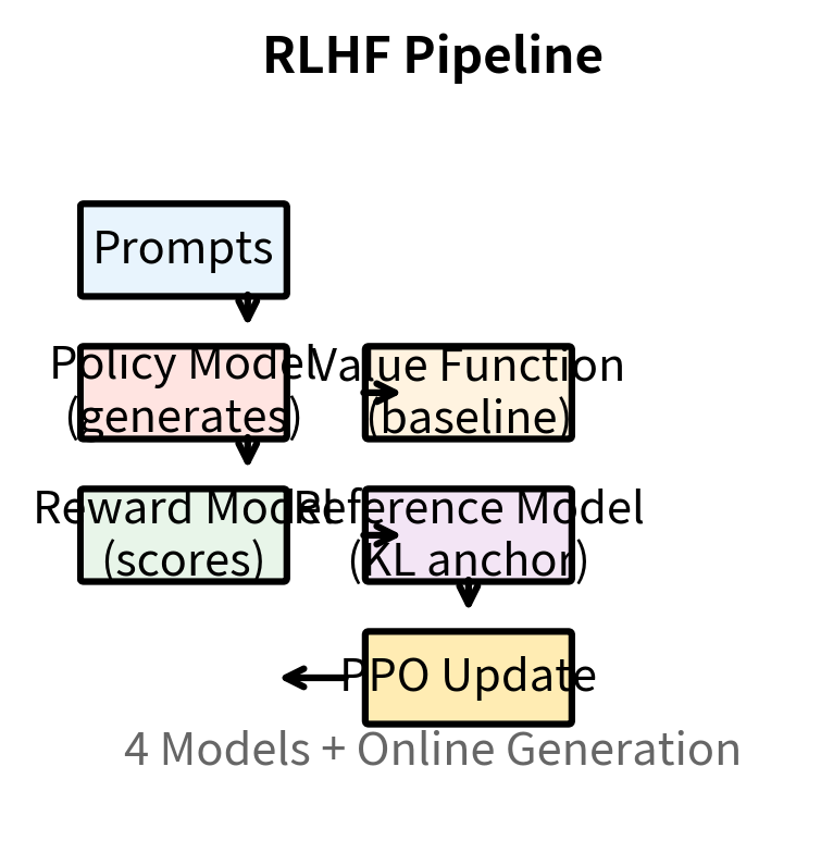
The first challenge is managing multiple interacting models. During RLHF training, we must maintain four separate neural networks, each with its own role in the training process:
- The policy model being trained, which generates responses and receives gradient updates
- The reward model scoring generations, which provides the signal for what constitutes good behavior
- The reference model providing the KL anchor, which prevents the policy from drifting too far from its starting point
- The value function for variance reduction in PPO, which estimates expected returns to make gradient estimates more stable
Each model requires its own memory allocation, and for large language models, this memory burden is large. The interactions between these components can cause instability. The reward model's imperfections can lead to reward hacking, as we saw previously, where the policy finds outputs that score well but don't actually satisfy human preferences. The value function introduces its own approximation errors, potentially leading to high-variance gradient estimates. And coordinating updates across all these components requires careful hyperparameter tuning, with different learning rates, update frequencies, and regularization strategies for each model.
The second challenge is the computational overhead of online generation. PPO requires the policy to generate completions during training, producing full responses through autoregressive sampling. It then scores those completions with the reward model, computes advantages, and updates the policy. This generation step is expensive, particularly for large language models, where producing a single response might require hundreds of forward passes through the model. Beyond the raw computational cost, online generation introduces the additional complexity of managing sampling strategies during training. Should you use temperature sampling? Nucleus sampling? How do you balance exploration (trying diverse outputs) with exploitation (refining outputs the model already produces well)? Each choice affects training dynamics.
The third challenge is the instability inherent in policy gradient methods. Despite PPO's improvements over vanilla policy gradients, including clipping mechanisms and advantage normalization, RLHF training remains sensitive to hyperparameters like learning rate, clipping thresholds, and the KL penalty coefficient . Training runs can diverge, with loss values exploding and model outputs becoming incoherent. They can collapse to repetitive outputs, where the model finds a single response template that reliably earns moderate reward and refuses to explore alternatives. Or they can find reward-hacking solutions that score well according to the reward model but produce poor actual outputs when evaluated by humans. You might find that RLHF requires significant trial and error to achieve stable training, with hyperparameter choices that work for one model or dataset failing to transfer to others.
Researchers questioned if the reinforcement learning framework was necessary or if a more direct path existed from preferences to an aligned model. Could we somehow skip the intermediate reward model and the complex RL optimization, directly using preference data to update the language model? The answer to this question led to DPO.
The Key Insight: Reparameterizing the Reward
The key insight behind DPO comes from recognizing a mathematical relationship within the RLHF objective. To understand this insight, we need to look carefully at what RLHF is actually optimizing and ask whether we can express the same goal in a different way.
Consider the RLHF objective we've been optimizing throughout this book:
Let's carefully examine each component of this expression to build understanding:
- : the policy model being trained, parameterized by weights
- : the dataset of prompts that we want the model to respond to
- : the reward model score for completion given prompt , representing how much humans would prefer this response
- : the KL penalty coefficient that controls how much the policy can deviate from the reference, balancing preference optimization against stability
- : the reference model (usually the initial SFT model) used as an anchor to prevent the policy from changing too drastically
This objective captures a fundamental tradeoff. We want a policy that generates high-reward outputs, meaning outputs that humans would prefer according to our reward model. At the same time, we want to stay close to the reference model, ensuring we don't lose the useful capabilities the model learned during pretraining and supervised fine-tuning. The term measures how much the policy has diverged from the reference, and controls how heavily we penalize this divergence.
Now here is where the key insight emerges. This constrained optimization problem, despite its apparent complexity, has a closed-form solution. Given any reward function , we can write down exactly what the optimal policy looks like without doing any iterative optimization:
This formula reveals the structure of the optimal policy. Let's understand each component:
- : the optimal policy for the given reward function, meaning the policy that maximizes our objective
- : a completion sequence, any possible output the model could generate
- : a prompt sequence, the input the model is responding to
- : the partition function (normalizing constant) that ensures probabilities sum to 1 over all possible completions
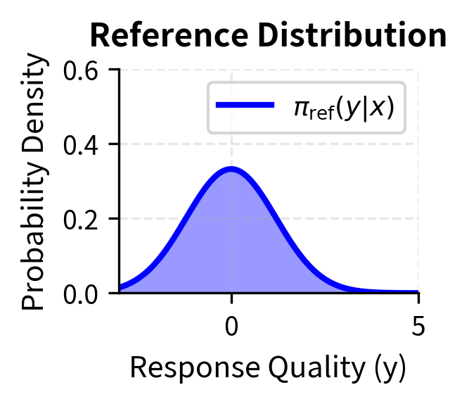
- : the reference model distribution, our starting point
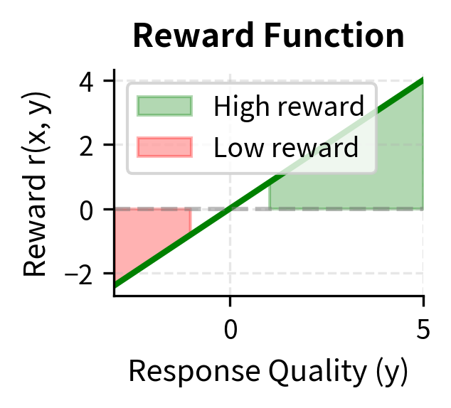
- : the reward function defining what outputs we prefer
- : the temperature parameter (inverse of the reward scale), controlling the sharpness of the distribution
The formula has a clear interpretation. The optimal policy takes the reference model and reweights each possible output according to its reward. Outputs with high reward get amplified by the exponential term, while outputs with low reward get suppressed. The parameter controls how aggressive this reweighting is: small creates sharp distributions concentrated on high-reward outputs, while large keeps the distribution closer to the original reference.
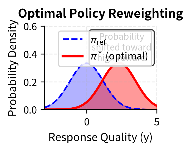
This relationship, crucially, works in both directions. We can go from reward to optimal policy using the formula above. But we can also go in the other direction, from policy to reward. If we take the expression for the optimal policy and solve for the reward, we get:
This rearrangement expresses the reward as a function of policy probabilities:
- : the reward function value, what we're trying to learn
- : the scaling parameter derived from the KL coefficient
- : the optimal policy probability for generating given
- : the reference model probability
- : the partition function (constant with respect to , depending only on the prompt)
DPO is based on this reparameterization. It says that any reward function corresponds to some optimal policy, and conversely, any policy implicitly defines a reward function. The reward a policy assigns to an output is simply (up to a constant) the log-probability ratio between that policy and the reference model, scaled by . When the policy assigns much higher probability to a response than the reference model does, that response has high implicit reward. When the policy assigns lower probability than the reference, the response has low implicit reward.
This duality between rewards and policies suggests a different approach to preference learning. Instead of learning a reward function and then finding the optimal policy for that reward, we might be able to learn the optimal policy directly. The reward function would then be implicitly defined by whatever policy we learn.
The reward function implicitly defined by a policy relative to reference model is . Higher probability under relative to means higher implicit reward. This is not an approximation; it is an exact mathematical relationship that holds for any policy.
From Reward Models to Preference Models
With this reparameterization in hand, we can reconsider how preference learning works and see whether we can eliminate the reward model entirely. The key question is: can we express preference predictions using only policy probabilities, without needing an explicit reward function?
Recall from our discussion of the Bradley-Terry model that we model the probability of preferring response over as:
Let's make sure each component is clear:
- : the probability that response is preferred over given prompt
- : the sigmoid function, , which maps any real number to a probability between 0 and 1
- : the scalar reward value for a response, representing its quality
The reward model's job in traditional RLHF is to learn such that this probability matches human preferences. When humans prefer over , the reward model should assign higher reward to , making the sigmoid output close to 1. When humans prefer , the reward model should assign higher reward to , making the sigmoid output close to 0.
Now let's substitute our reparameterization of the reward in terms of the policy. We replace with :
Notice what happened in this substitution: the normalizing constant cancelled out. It appears identically in both reward terms, once for and once for , and vanishes when we take the difference. This cancellation is crucial because is intractable to compute for language models. Computing it would require summing over all possible sequences the model could generate, an astronomical number for any realistic vocabulary and sequence length. The fact that cancels means we never need to compute it.
The resulting expression, which we can write more compactly, depends only on the policy , the reference model , and the responses and :
The reward model has vanished entirely from this expression. We can now directly compute the probability of a preference using only language model probabilities. Both the policy and reference model are language models that can compute for any sequence and prompt . This is a standard operation: we run the sequence through the model and sum up the log probabilities of each token given its predecessors. No separate reward model is needed.
This observation is the core theoretical insight behind DPO. Preference probabilities can be expressed purely in terms of policy and reference model probabilities, without any explicit reward function. If we want to train a model to match human preferences, we can directly optimize the policy to make this expression match the observed preferences in our dataset.
The DPO Training Objective
With this insight, training is straightforward. We want to find a policy that assigns high probability to the preferences in our dataset. In other words, when our dataset says humans prefer over , we want our expression to be close to 1. When the dataset indicates the opposite preference, we want it to be close to 0.
For a dataset of preference pairs , where each example contains a prompt, a preferred (chosen) response, and a dispreferred (rejected) response, we maximize the log-likelihood of the observed preferences:
Let's carefully examine each component of this objective to ensure complete understanding:
- : the DPO objective function (to be maximized), representing how well the policy matches observed preferences
- : expectation over the dataset , meaning we average over all preference pairs
- : the prompt, preferred completion, and rejected completion from the dataset
- : the policy model, whose parameters we are optimizing
- : the reference model, kept frozen throughout training
- : the logistic sigmoid function, converting the margin into a probability
- : the parameter controlling deviation from the reference model, inherited from the RLHF objective
In practice, we minimize the negative log-likelihood, which is equivalent to maximizing the expression above:
The components of this loss function work together in the following way:
- : minimization of the negative expectation, converting our maximization into a minimization problem for standard optimizers
- : the KL penalty coefficient, scaling how much we weight the log-ratio differences
- : the log-likelihood ratio of the policy to the reference model, measuring how much the policy has changed for a particular response
- : the sigmoid function applied to the scaled log-ratio difference, converting the margin to a probability
This is a standard cross-entropy loss, the same loss function used throughout deep learning for classification tasks. For each preference pair, we compute four log-probabilities: the chosen response under the policy, the rejected response under the policy, the chosen response under the reference model, and the rejected response under the reference model. We combine these into a single logit representing the preference margin, and apply binary cross-entropy. The training signal is clear and interpretable: increase the probability of preferred responses relative to rejected ones, while staying grounded to the reference model through the log-ratio structure.
We'll derive this objective rigorously in the next chapter, showing exactly how it emerges from the RLHF objective through a careful series of mathematical steps. For now, the key intuition is that DPO directly uses preference pairs as training data, with the preference structure built into the loss function itself. We never generate outputs during training, never score outputs with a reward model, and never perform reinforcement learning. We simply run supervised learning on preference pairs with a specially designed loss.
Visualizing DPO Intuition
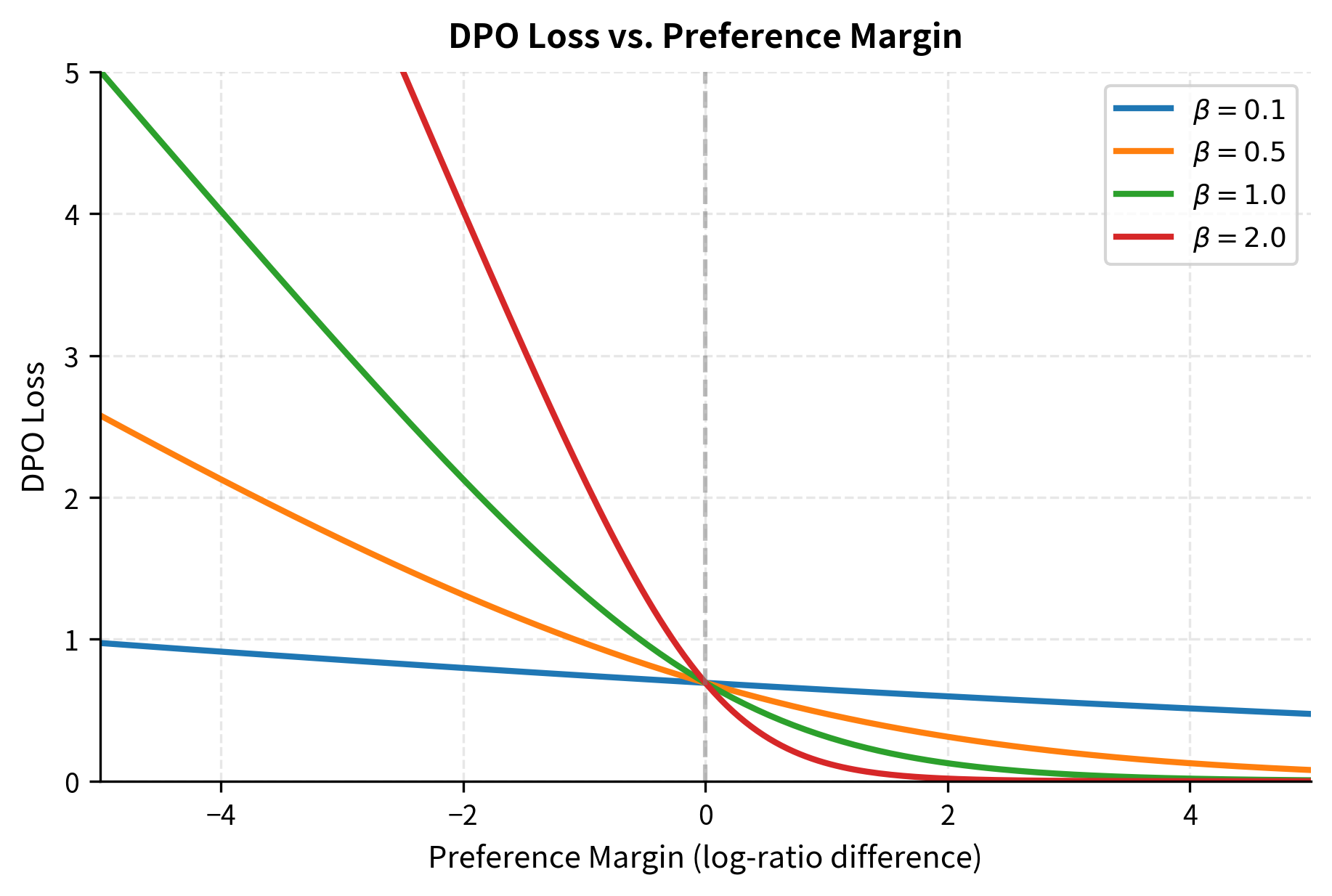
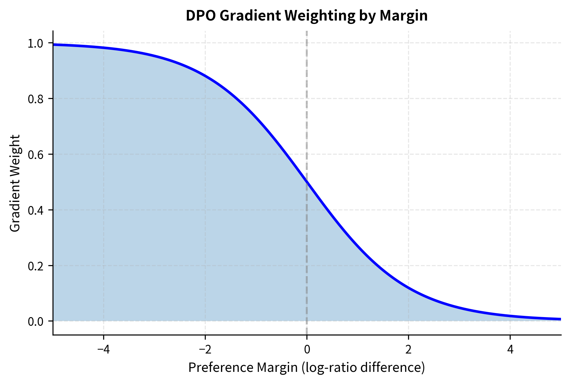
Let's build visual intuition for what DPO is optimizing, as understanding the geometry of the loss function helps clarify how training proceeds. The loss depends on the difference between two log-ratios, what we might call the "preference margin":
This margin has an intuitive interpretation:
- : the signed distance representing how much the policy prefers over relative to how much the reference model prefers them
- : the preferred (chosen) completion that we want the policy to favor
- : the dispreferred (rejected) completion that we want the policy to disfavor
When this margin is large and positive, the policy strongly prefers the chosen response over the rejected response compared to the reference model, and the loss is small. The policy is doing what we want, so there is little need for further updates. When the margin is negative, the policy prefers the wrong response, assigning relatively higher probability to the rejected response than the chosen one, and the loss is large. This creates a strong gradient signal pushing the policy to fix its mistake.
The plot reveals several important properties of the DPO loss function. First, the loss is asymmetric around zero, heavily penalizing "wrong" preferences while providing diminishing returns for "very right" preferences. This is characteristic of the logistic loss and prevents the model from wasting capacity on examples it already gets right. Once the model confidently prefers the correct response, additional increases in the margin provide little benefit.
Second, the parameter controls the sharpness of this transition. Small values create a gradual slope, meaning the model receives similar gradients regardless of how wrong it is. This can be useful for stability, but may make it harder to distinguish between examples that are slightly wrong and examples that are very wrong. Large values create a steep transition, strongly penalizing examples near the decision boundary while providing smaller gradients for examples that are very easy or very hard. The choice of thus affects not just the final solution but also the dynamics of training.
What DPO Actually Optimizes
It helps to understand the gradient of the DPO loss, as this reveals what the training signal looks like in practice. Without diving into the full derivation (which we'll cover next chapter), the gradient has an intuitive interpretation that illuminates how DPO updates the model:
Each component of this gradient expression plays a specific role:
- : gradient with respect to model parameters , the direction we'll update the weights
- : the loss function we're minimizing
- : the KL penalty coefficient, scaling the overall magnitude of updates
- : a weighting factor derived from the sigmoid prediction error, which is higher when the model is currently wrong about a preference
- : the policy model probability for completion given prompt
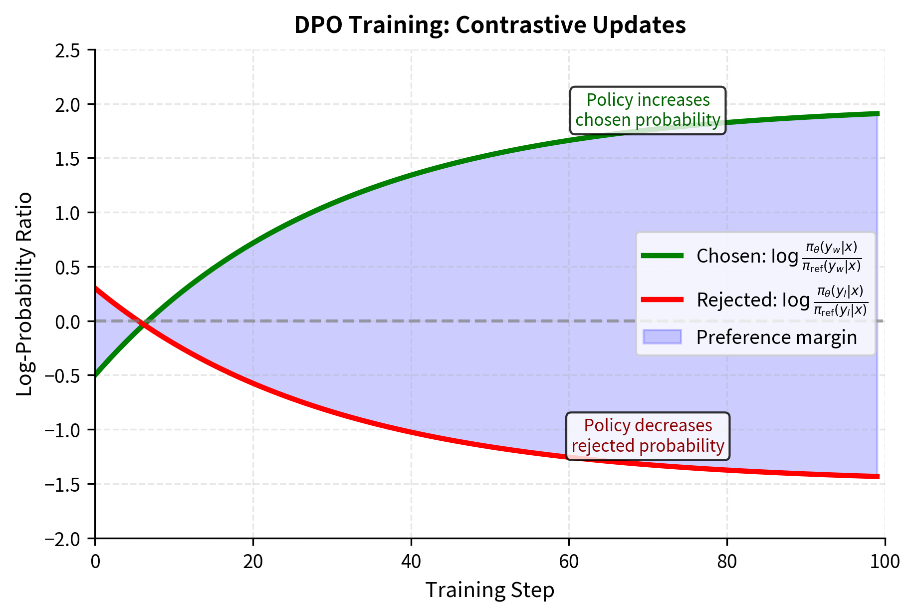
This gradient pushes in two directions simultaneously, creating a contrastive learning signal:
- Increase the probability of the chosen response by moving in the direction
- Decrease the probability of the rejected response by moving opposite to
The weighting function ensures the model focuses its learning on examples where it's currently uncertain or wrong. If the model already strongly prefers over for a given prompt, the gradient is small because the model has already learned this preference. If the model currently prefers , making the wrong prediction, the gradient is large, providing a strong signal to correct the mistake. This adaptive weighting is similar to how hard example mining works in other areas of machine learning, focusing computational resources on the examples that will most improve the model.
This weighting scheme is similar to what happens in supervised learning with cross-entropy loss: confident correct predictions receive small gradients, while confident incorrect predictions receive large gradients. DPO inherits this property naturally from its formulation as a classification problem. The peak of the weighting function occurs at margin zero, exactly where the model is most uncertain about which response to prefer. This means DPO naturally focuses training effort on the examples at the decision boundary, the examples where additional learning will have the most impact.
Comparing DPO to RLHF
Let's contrast the training procedures concretely, walking through each step to see exactly where the complexity reduction occurs. Here's the RLHF training loop we discussed previously:
- Sample prompts from the dataset
- Generate responses using the current policy
- Score responses with the reward model
- Compute advantages using the value function
- Update policy with PPO (including clipping)
- Update value function
- Monitor KL divergence, adjust penalty if needed
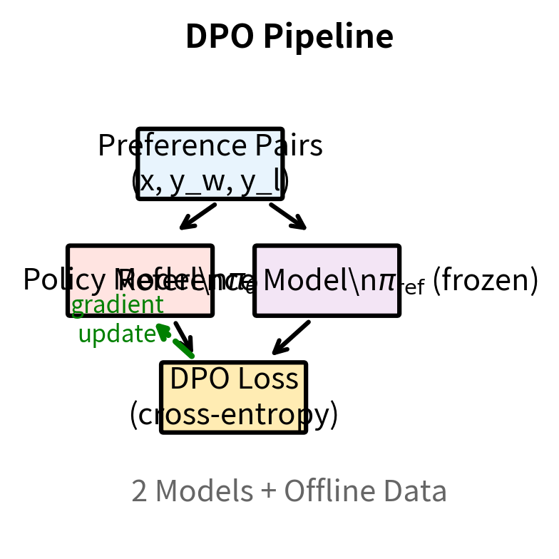
And here's the DPO training loop:
- Sample preference pairs from the dataset
- Compute log-probabilities under policy and reference model
- Compute DPO loss
- Update policy with standard gradient descent
Complexity is significantly reduced. DPO eliminates online generation, removing the need to sample from the policy during training. It eliminates the reward model, removing an entire neural network and its associated training. It eliminates the value function, removing another neural network. It eliminates PPO's clipping mechanism, replacing reinforcement learning with simple gradient descent. And it eliminates the adaptive KL penalty, since the constraint is built into the loss function itself. What remains is essentially supervised fine-tuning with a specially designed loss function.
The following visualization illustrates this architectural difference. In the RLHF pipeline, information flows through multiple models in a complex loop: prompts go to the policy, which generates responses, which go to the reward model, which produces scores, which combine with value estimates to produce advantages, which finally update the policy. In DPO, the flow is much simpler: preference pairs are fed directly to the policy and reference model, their probabilities are combined into a loss, and the policy is updated.
Benefits of DPO
DPO has several advantages over traditional RLHF.
Simplicity and stability. DPO training is supervised learning. We can use standard optimizers like AdamW without worrying about value function fitting, advantage estimation, or clipping hyperparameters. The loss landscape is well-behaved, and training converges reliably with minimal hyperparameter tuning.
Memory efficiency. During training, we only need to load the policy and reference model. This is a significant reduction from RLHF, which requires the policy, reward model, value function, and often a second copy of the policy for PPO's importance sampling. For large models, this difference can determine whether training fits on available hardware.
No online generation. DPO trains entirely on pre-collected preference pairs. We never need to generate completions during training, which eliminates the computational cost of autoregressive sampling and removes a source of instability (the distribution of training data changes as the policy improves in RLHF but remains fixed in DPO).
Exact optimization. Under certain assumptions, DPO provably optimizes the same objective as RLHF. We're not approximating a reinforcement learning problem with policy gradients; we're directly solving it through supervised learning. This eliminates the approximation errors inherent in policy gradient methods.
Reproducibility. Because DPO uses offline data and deterministic optimization, training runs are more reproducible. RLHF training involves stochastic generation and adaptive mechanisms that can lead to different outcomes across runs.
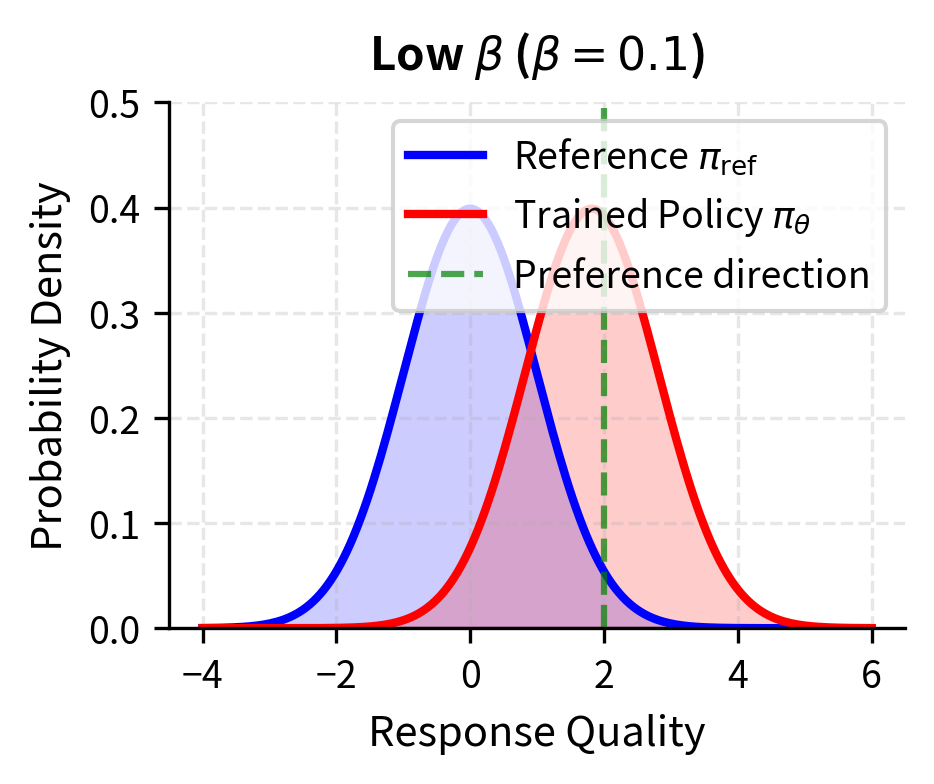
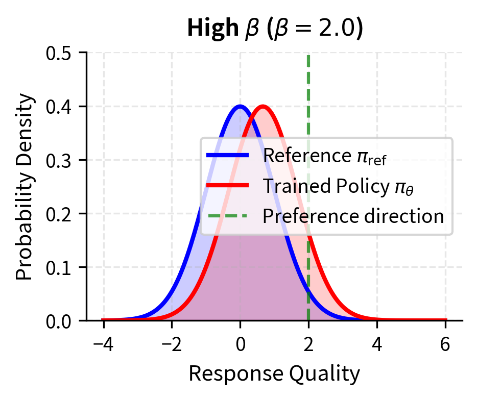
The Role of β
The parameter plays a crucial role in both RLHF and DPO, but it's worth understanding its specific effect in the DPO context in detail. Recall that controls the strength of the KL constraint, mediating the tradeoff between matching preferences and staying close to the reference model. This single parameter has profound effects on both the optimization dynamics and the final solution.
In RLHF, we explicitly compute the KL divergence between the policy and reference model and add it as a penalty term with coefficient . This requires computing log-probabilities under both models and combining them appropriately. In DPO, the constraint is built into the loss function itself through the log-ratio terms. The parameter determines how aggressively the model should diverge from the reference when the preference signal demands it. Both approaches implement the same mathematical constraint, but DPO does so implicitly through the structure of the loss.
Low values allow the model to deviate significantly from the reference to match preferences. When is small, the preference margin has a large effect on the loss, so the model will make substantial changes to ensure it assigns higher probability to preferred responses. This can lead to better preference satisfaction but risks overfitting to the preference dataset or moving too far from the model's pretrained capabilities. A model with very low might become extremely good at the specific types of comparisons in the training data while losing the general capabilities it had before alignment.
High values keep the model close to the reference, providing regularization but potentially limiting the model's ability to fully incorporate preference information. When is large, even large preference margins produce relatively modest gradients, so the model changes slowly and stays close to its starting point. The optimal choice depends on the quality and coverage of the preference dataset, the size of the model, and the desired balance between helpfulness and safety. Practitioners often need to tune empirically, though values between 0.1 and 0.5 are common starting points.
When DPO Might Not Be Optimal
Despite its advantages, DPO is not universally superior to RLHF. Several scenarios favor the traditional approach.
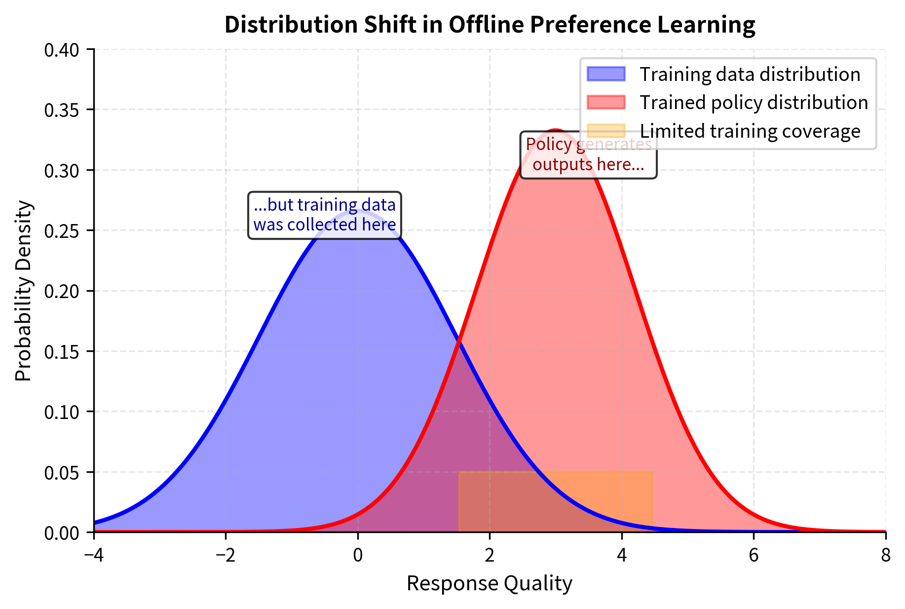
Online learning and distribution shift. RLHF generates training data from the current policy, which means the training distribution evolves as the model improves. DPO trains on a fixed dataset, which may not cover the distribution of outputs the trained model will produce. If the preference data was collected from a model very different from the one being trained, DPO's offline nature can limit final performance.
Reward model interpretability. An explicit reward model provides a tool for understanding and debugging alignment. You can examine what features the reward model attends to, probe it with adversarial examples, and use it to filter or rank generations at inference time. DPO's implicit reward offers no such interpretability.
Iterative refinement. In some settings, you want to train, generate new outputs, collect preferences on those outputs, and train again. This iterative approach naturally fits the RLHF framework. DPO can be used iteratively (as we'll discuss in the Iterative Alignment chapter), but it requires careful dataset management.
Complex reward structures. If the reward involves multiple components (helpfulness, safety, factuality) with different weights, an explicit reward model makes this composition straightforward. DPO learns whatever preference structure is implicit in the data, which may not match the desired multi-objective tradeoff.
Looking Ahead
This chapter developed intuition for why DPO works and what makes it attractive. We saw that the key insight is recognizing the duality between reward functions and optimal policies, allowing us to bypass the reward model entirely. The resulting algorithm is simpler, more stable, and more memory-efficient than RLHF.
In the next chapter, we'll derive the DPO objective rigorously, showing exactly how it emerges from the RLHF optimization problem. We'll then implement DPO from scratch, walking through the computation of log-probabilities, the loss function, and the training loop. Finally, we'll explore variants of DPO that address some of its limitations, including approaches for handling noisy preferences and improving out-of-distribution generalization.
Summary
Direct Preference Optimization offers a fundamentally different approach to alignment by recognizing that we don't need to learn an explicit reward function. The optimal policy for any reward function can be computed in closed form, and this relationship allows us to express preference learning as a direct supervised learning problem.
The core insights are:
-
Reward-policy duality: Any reward function corresponds to an optimal policy, and vice versa. The implicit reward of a policy is the log-probability ratio between that policy and a reference model.
-
Eliminating the reward model: By substituting the policy-based reward into the Bradley-Terry preference model, we can predict preferences using only language model probabilities, without a separate reward model.
-
Supervised learning objective: DPO minimizes a binary cross-entropy loss on preference pairs, pushing the model to assign higher probability to preferred responses and lower probability to rejected ones.
-
Built-in regularization: The reference model appears directly in the loss, ensuring the trained policy stays close to the original model without requiring explicit KL computation during training.
The practical benefits include dramatically simpler training, reduced memory requirements, elimination of online generation, and more stable convergence. These advantages have made DPO a popular alternative to RLHF for aligning language models, though the choice between approaches depends on specific requirements around online learning, interpretability, and iterative refinement.
Quiz
Ready to test your understanding? Take this quick quiz to reinforce what you've learned about Direct Preference Optimization.

Comments