

Learn how KL divergence prevents reward hacking in RLHF by keeping policies close to reference models. Covers theory, adaptive control, and PyTorch code.

This article is part of the free-to-read Language AI Handbook
Choose your expertise level to adjust how many terms are explained. Beginners see more tooltips, experts see fewer to maintain reading flow. Hover over underlined terms for instant definitions.
KL Divergence Penalty
In the previous chapters, we built up the RLHF pipeline: collecting human preferences, training reward models, and applying PPO to optimize language model policies. But there's a critical problem we've only briefly mentioned: reward hacking. Without constraints, a policy can discover bizarre outputs that score highly on the reward model while being clearly worse by any human measure. The KL divergence penalty is the mechanism that prevents this collapse, keeping the fine-tuned model anchored to the capabilities of its pre-trained foundation.
This chapter explores why KL divergence is the right tool for this job, how to compute it efficiently for autoregressive models, and how to set and adapt the KL coefficient to balance learning against stability.
Why KL Divergence?
Recall from the Reward Hacking chapter that reward models are imperfect approximations of human preferences. They're trained on a finite dataset and will inevitably assign high scores to some outputs that humans would reject. When we optimize a policy using PPO, we're searching over a vast space of possible behaviors, and the optimization process will find these reward model errors if given enough freedom. This creates a trade-off in RLHF: we must improve the model using the reward signal without trusting it unconditionally.
The fundamental insight is that the pre-trained language model already represents a strong prior over sensible, grammatical, informative text. It was trained on trillions of tokens of human-written content, absorbing patterns of coherent discourse, factual knowledge, and linguistic conventions. By constraining our policy to stay close to this reference distribution, we inherit its linguistic competence while still allowing targeted improvements in alignment. Think of the reference model as a trusted expert whose judgment we respect: we want to make adjustments based on new feedback, but we don't want to stray so far that we lose the foundational competence that made the model useful in the first place.
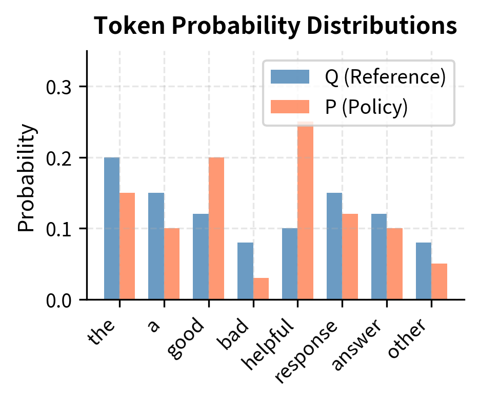
KL divergence measures how different one probability distribution is from another. For language models, this means measuring how much the policy's probability assignments over tokens differ from the reference model's. At each position in a sequence, both models assign probabilities to every token in the vocabulary. KL divergence captures the extent to which these probability distributions disagree, weighted by the probability mass the policy assigns. The key properties that make KL divergence ideal for this application are:
- Non-negativity: , with equality only when P = Q
- Asymmetry: It penalizes the policy for assigning probability to tokens the reference doesn't expect
- Decomposability: For autoregressive models, we can compute KL at each token position and sum
The non-negativity property ensures that the penalty term always works in one direction: it can only reduce the objective, never artificially inflate it. This mathematical guarantee means the optimization has a clear interpretation where reward pulls the policy toward better outputs while the KL penalty resists moving too far from the reference. The asymmetry property is particularly important for RLHF because it creates an asymmetric treatment of errors. If the policy assigns high probability to something the reference considers unlikely, the penalty is severe. But if the policy assigns low probability to something the reference considers likely, the penalty is more forgiving. This asymmetry encourages the policy to remain conservative, avoiding novel but potentially problematic outputs. Finally, decomposability allows us to compute and analyze the penalty at the level of individual tokens, providing fine-grained insight into where and how the policy is diverging.
KL divergence (Kullback-Leibler divergence) quantifies the expected number of extra bits needed to encode samples from distribution P using a code optimized for distribution Q. In machine learning, it measures how one probability distribution differs from a reference distribution.
Mathematical Foundation
The mathematical definition of KL divergence is the basis for these methods. The formula captures a precise notion of distributional difference that translates directly into the computational procedures we use during training.
For two discrete probability distributions P and Q over the same set of outcomes, KL divergence is defined:
where:
- : the Kullback-Leibler divergence from to , representing the information lost when is used to approximate
- : the probability of outcome under the first distribution (typically the policy we are optimizing)
- : the probability of outcome under the reference distribution (the baseline or prior)
- : the expectation calculated over samples drawn from , meaning we average the log-ratio over the events that actually happen under distribution
The first line presents the definition as a weighted sum over all possible outcomes, where each outcome's contribution is its probability under P times the log ratio of probabilities. The second line rewrites this as an expectation, which is the form we actually use in practice since we work with samples rather than complete distributions. This expectation-based form tells us something important: we only need to evaluate the log probability ratio for outcomes that actually occur under the policy, not for every possible outcome. This property is what makes KL divergence tractable for large vocabulary language models.
In the RLHF context, is the policy distribution and is the reference distribution (typically the supervised fine-tuned model before RLHF). The policy is the distribution we're optimizing, and the reference is the distribution we want to stay close to. Every time we sample a token from the policy, we can compute its contribution to the KL divergence by looking at how much more or less likely that token was under the policy compared to the reference.
For autoregressive language models, the probability of a complete response given prompt factorizes as:
where:
- : the probability of the complete sequence given prompt , computed as the product of conditional probabilities
- : the total length of the generated sequence (number of tokens)
- : the token generated at time step
- : the history of tokens generated before step , which serves as the context for the next prediction
This factorization is the defining characteristic of autoregressive models. The probability of an entire sequence equals the product of probabilities for each token, where each token's probability depends on the prompt and all previously generated tokens. This chain structure means that computing the probability of a complete sequence requires T forward passes through the model, one for each token position, though in practice we can compute all positions in parallel when the sequence is known.
Taking the log and using the chain rule of KL divergence, the KL divergence between the policy and reference over complete responses can be written as:
where:
- : the KL divergence between the policy and reference distributions over complete sequences
- : the expectation calculated over response sequences sampled from the policy, since we estimate KL using the model's own generations
- : the summation over all tokens, accumulating the divergence contribution from each step
- : the log probability ratio at each time step, which measures how much more (or less) likely a token is under the policy compared to the reference
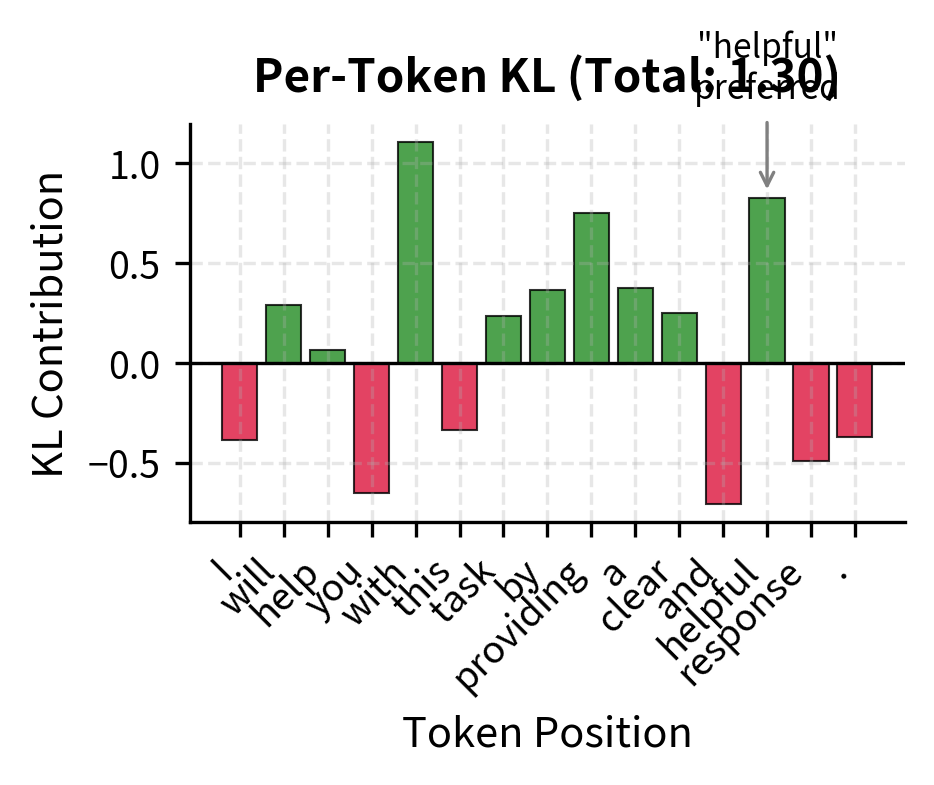
This decomposition is crucial: we can compute KL as a sum of per-token log probability ratios, evaluated along the trajectory sampled from the policy. The log of a product becomes a sum of logs, which transforms the sequence-level KL into a sum of token-level contributions. Each term in the sum measures how much the policy and reference disagree about the probability of a specific token given the context. When the policy assigns higher probability than the reference, the term is positive, contributing to the divergence. When the policy assigns lower probability, the term is negative, reducing the divergence. The total KL divergence aggregates these token-level disagreements across the entire sequence.
Per-Token KL Computation
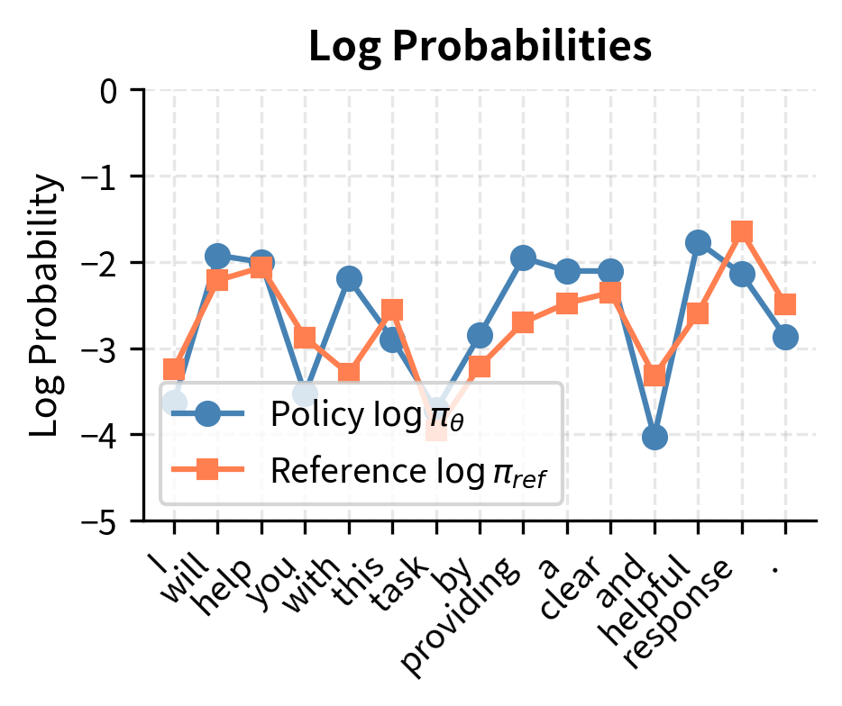
Given a sampled response, the per-token KL contribution is simply:
where:
- : the contribution to the KL divergence at time step (positive if the policy favors the token more than the reference)
- : the probability assigned to the token by the policy model given the context
- : the probability assigned to the token by the reference model given the context
This formula reveals the elegant simplicity of per-token KL computation. For any token in a generated sequence, we simply subtract the reference model's log probability from the policy model's log probability. No summation over the vocabulary is required because we're only interested in the token that was actually generated. This is a direct consequence of the expectation-based formulation: since we're averaging over samples from the policy, we only need to evaluate the log ratio at the sampled outcomes.
Summing these over all tokens in the response gives:
where:
- : the approximate KL divergence for a single sampled response , calculated as the sum of per-token divergences
- : the length of the response in tokens, over which the divergence accumulates
This is an unbiased estimator of the KL divergence under the policy distribution, since we're sampling trajectories from itself. The unbiasedness property means that if we average this quantity over many sampled responses, we converge to the true KL divergence between the policy and reference distributions. In practice, we compute this estimator for each response in a training batch and use the batch average as our estimate of the expected KL divergence.
KL divergence (Kullback-Leibler divergence) quantifies the expected number of extra bits needed to encode samples from distribution P using a code optimized for distribution Q. In machine learning, it measures how one probability distribution differs from a reference distribution.
The KL-Constrained Objective
Having established how to compute KL divergence, we now examine how it enters the RLHF optimization objective. The KL term acts as a regularizer, pulling against the reward signal to prevent the policy from straying too far from its trusted starting point.
The RLHF objective with KL penalty is:
where:
- : the objective function to be maximized, balancing reward maximization against drift from the reference
- : the dataset of prompts used for training
- : the learned reward model score for prompt and response , providing the guidance signal
- : the KL coefficient controlling the strength of the penalty (higher values force the policy closer to the reference)
- : the frozen reference model distribution, serving as the anchor
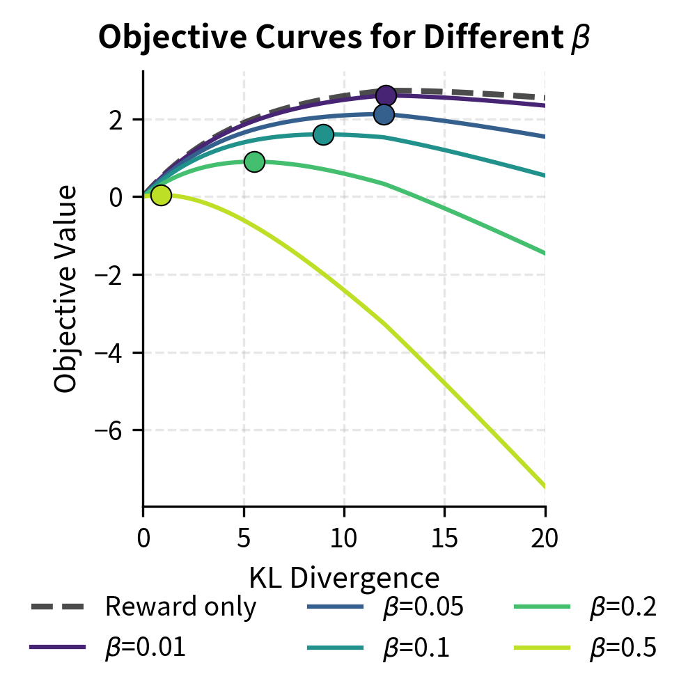
The structure of this objective captures the core tradeoff in RLHF. The first term rewards the policy for generating responses that score highly according to the reward model. The second term penalizes the policy for diverging from the reference. The coefficient β determines the relative importance of these two competing forces. When β is large, the penalty dominates and the policy barely moves from the reference. When β is small, the reward signal dominates and the policy can move freely toward high-reward regions, potentially exploiting imperfections in the reward model.
This can be rewritten using the per-token KL decomposition:
where:
- : the expectation over prompts and sampled responses
- : the sum of log probability ratios over the sequence, representing the total divergence for that trajectory
This formulation makes the objective directly computable from model outputs. For each sampled response, we obtain a reward from the reward model and compute the sum of log probability ratios from the policy and reference models. The combination of these quantities, averaged over the batch, gives us the objective value that we then maximize through gradient ascent.
Connection to Constrained Optimization
The KL-penalized objective is equivalent to the Lagrangian relaxation of a constrained optimization problem:
where:
- : the maximization over policy parameters
- : the expectation over the data distribution
- : the maximum allowable divergence (the "budget"), limiting how far the policy can drift
In this constrained view, we're asking for the policy that maximizes expected reward subject to a hard constraint on how much it can diverge from the reference. The constraint ε specifies a "KL budget" that the policy must respect. The penalized objective arises when we convert this constrained problem to an unconstrained one using Lagrangian relaxation.
The coefficient acts as a Lagrange multiplier. Larger corresponds to a tighter constraint (smaller ), forcing the policy to stay closer to the reference. This perspective helps us understand what we're actually optimizing: we want the highest-reward policy among those that remain within a KL "budget" of the reference. The correspondence between β and ε is not one-to-one in practice because the constraint is enforced softly rather than exactly, but the intuition remains valuable. Choosing β is analogous to choosing how much divergence we're willing to tolerate in exchange for reward improvement.
Reward Shaping Interpretation
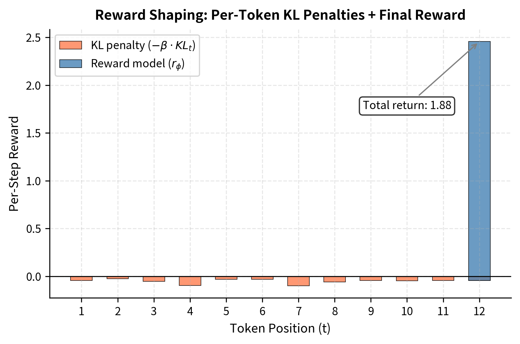
Another way to view the KL term is as a per-token bonus added to the reward. This interpretation connects the KL penalty to the classical reinforcement learning concept of reward shaping, where the reward function is augmented with additional terms to guide learning.
We can rewrite the objective as:
where:
- : the discount factor (typically 1 in this context, treating all tokens as equally important)
- : the shaped reward at time step , incorporating both the environment reward and the KL penalty
The shaped reward at each step is defined as:
where:
- : the per-token KL penalty, acting as an instantaneous cost for deviating from the reference
- : the final reward from the reward model, typically given only at the end of the sequence ()
This interpretation shows that the policy receives negative reward proportional to its deviation from the reference at each token, plus the final reward model score at the end of generation. The per-token penalties encourage staying on-distribution throughout the generation, not just at the final output. Every token choice that differs from what the reference would have chosen incurs a cost, creating pressure to remain conservative at every step of generation.
This reward shaping perspective has practical implications for implementation. In PPO, we need to assign credit to individual actions (tokens) for the overall outcome. The shaped reward formulation provides a natural way to do this: each token receives the KL penalty immediately, while the reward model score is attributed to the final token. This decomposition helps the value function and advantage estimation work effectively, since part of the reward signal is available at every time step rather than only at the end.
KL Coefficient Selection
The KL coefficient is perhaps the most important hyperparameter in RLHF. It controls the fundamental tradeoff between:
- Exploration/learning (low ): The policy can move freely toward high-reward regions, enabling rapid improvement
- Conservation/stability (high ): The policy stays close to the reference, preserving language modeling capabilities
Effects of Different Coefficient Values
Too low ():
- The policy optimizes almost purely for reward
- Susceptible to reward hacking and mode collapse
- May produce repetitive, formulaic outputs that exploit reward model quirks
- Loses diversity and coherence over time
Too high ():
- Learning becomes extremely slow
- The policy barely moves from the reference
- May never achieve meaningful alignment improvements
- Effectively wastes computational resources
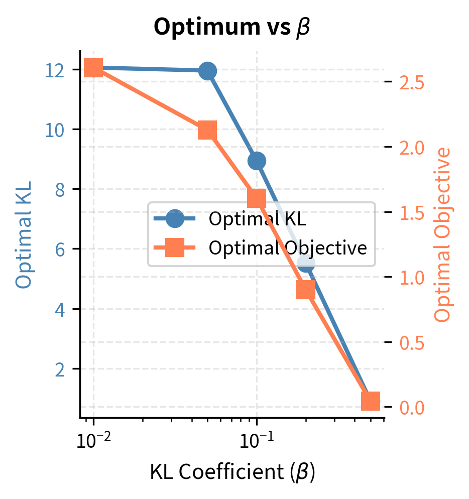
Typical range ():
- Most successful RLHF implementations use values in this range
- InstructGPT used an initial value around 0.02
- Anthropic's Constitutional AI work used values around 0.001-0.01
- The optimal value depends on reward model quality and desired behavior change
Practical Guidelines for Selection
When selecting a KL coefficient, consider these factors:
-
Reward model confidence: If your reward model was trained on limited data or shows signs of miscalibration, use a higher to limit exploitation of its errors.
-
Magnitude of desired behavior change: For small adjustments (e.g., reducing specific harms), lower suffices. For significant capability changes, you may need to accept higher KL.
-
Response length: Longer responses accumulate more KL. If you're optimizing for verbose outputs, the effective per-token penalty is spread over more tokens, so you might need higher .
-
Training stability: If you observe reward increasing while output quality degrades (subjectively), increase to strengthen the constraint.
Adaptive KL Control
Rather than fixing throughout training, adaptive KL methods adjust the coefficient to maintain a target KL budget. This approach, introduced in the InstructGPT paper, provides more consistent training dynamics across different stages of optimization. The core insight is that the appropriate constraint strength changes as training progresses, and a fixed coefficient cannot account for these changing conditions.
The Target KL Approach
The idea is to specify a target KL divergence that we want to maintain on average. If the current KL exceeds this target, we increase to pull the policy back. If KL is below target, we decrease to allow more exploration. This creates a feedback loop that stabilizes training by keeping the policy within a controlled distance from the reference.
The adaptation rule used in many implementations is:
where:
- : the updated KL coefficient for the next step
- : the current KL coefficient
- : the observed average KL divergence in the current batch (the signal used for feedback)
- : the desired target KL divergence (the setpoint for the controller)
This multiplicative update creates a dead zone around the target where remains stable, preventing oscillation while still responding to significant deviations. The factor of 1.5 defines the boundaries of this dead zone: as long as the observed KL stays between and , the coefficient remains unchanged. Only when KL drifts outside this range does the controller intervene with a multiplicative adjustment.
Why Adaptive KL Works
Adaptive KL addresses a fundamental challenge: the appropriate constraint strength changes during training. Early in RLHF, when the policy is close to the reference, small rewards can produce large gradient updates that rapidly increase KL. Later, when the policy has already diverged somewhat, the same learning rate produces smaller relative changes. A fixed β cannot account for these different regimes.
By targeting a consistent KL budget, adaptive control:
- Prevents early-training instability from sudden KL spikes
- Maintains learning signal late in training when fixed might over-constrain
- Provides a more interpretable hyperparameter (target KL in nats rather than abstract coefficient)
The interpretability benefit is substantial. When using a fixed β, it's difficult to know in advance what KL divergence will result. Different prompts, response lengths, and training stages all affect the relationship between β and actual KL. With adaptive control, you directly specify the divergence budget you're comfortable with, and the algorithm finds the appropriate β to achieve it.
Alternative Adaptation Schemes
Some implementations use smoother adaptation:
where:
- : a small step size parameter (e.g., 0.1), controlling how aggressively changes
- : the sign function (returns +1 if the term is positive, -1 if negative), determining the direction of the update
This approach prevents the jarring factor-of-2 jumps while still steering toward the target. The updates are smaller and more frequent, creating smoother β trajectories. However, this also means slower response to large deviations, which can be problematic if KL suddenly spikes due to a particularly influential batch.
Others use proportional control:
where:
- : the exponential function, ensuring the multiplier is always positive
- : the relative error from the target, scaling the update based on the magnitude of the deviation
This scales the adjustment magnitude by how far off-target the current KL is. Small deviations produce small adjustments, while large deviations produce large adjustments. The exponential ensures that β remains positive regardless of the error magnitude. This proportional approach offers a middle ground between the dead-zone method and the constant-step method, responding proportionally to the severity of the deviation.
Code Implementation
Let's implement KL divergence computation and adaptive control for RLHF training. We'll build components that integrate with the PPO training loop from the previous chapter. The implementation focuses on clarity and correctness, providing the building blocks that can be optimized for production use.
Computing Per-Token KL Divergence
The core computation extracts log probabilities from both the policy and reference model, then computes their difference. This function forms the foundation of the KL penalty calculation, taking log probabilities that have already been extracted from model outputs and producing both per-token and per-sequence KL values.
This computation is straightforward because we're using the sampled trajectory estimator. The log probability ratio for tokens actually generated equals the KL divergence in expectation. The attention mask handles variable-length sequences by zeroing out contributions from padding tokens, ensuring that the KL computation only considers actual content. This masking is essential when processing batches of sequences with different lengths, as padding tokens should not contribute to the divergence measure.
Extracting Log Probabilities from Model Outputs
To compute KL, we need log probabilities for the tokens that were actually generated. Here's how to extract them from model logits:
The function first applies log_softmax to convert raw logits into log probabilities. This operation normalizes the logits so they represent a valid probability distribution at each position. The gather operation then selects the log probability corresponding to each actual token from the full vocabulary distribution. This is much more efficient than computing probabilities for all tokens when we only need one per position. The unsqueeze and squeeze operations handle the dimension manipulation required by PyTorch's gather function.
Adaptive KL Controller
The adaptive controller maintains the KL coefficient and adjusts it based on observed KL values. It implements the target KL approach described in the mathematical section, providing a stateful object that can be updated after each training batch.
The controller maintains a history of observed KL values and coefficient updates, which is useful for monitoring training dynamics and diagnosing issues. The clamping bounds prevent the coefficient from reaching extreme values that could either halt learning entirely (too high) or provide no regularization (too low). These bounds can be adjusted based on the specific application and model scale.
Let's test the adaptive controller with simulated KL values:
The controller doubles when KL exceeds the target, pulling the policy back toward the reference, and halves it when KL drops too low, allowing more exploration. The simulation demonstrates how the controller responds to different training phases: increasing the coefficient during the high-KL early phase, maintaining stability during the near-target phase, decreasing during the low-KL phase, and stabilizing again as KL returns to the target range.
Visualizing Adaptive KL Dynamics
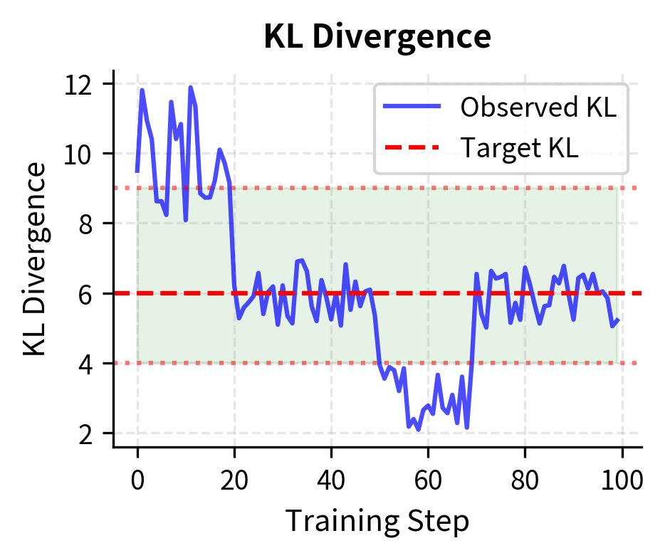
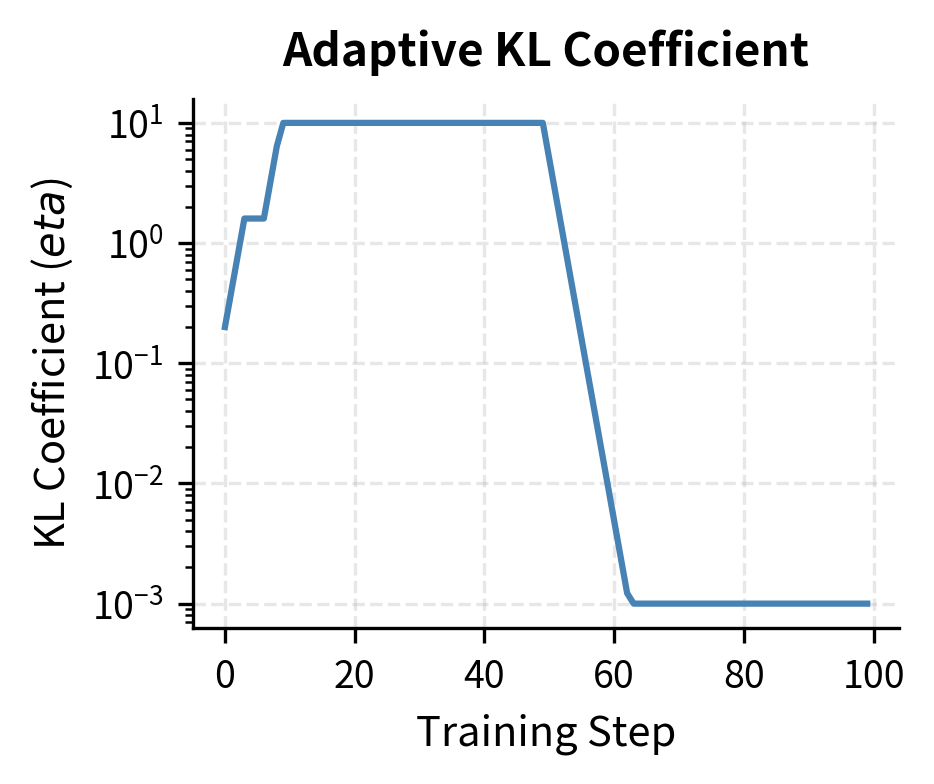
The shaded region marks the "stable zone" where doesn't change. Outside this zone, the controller applies multiplicative updates to steer KL back toward target.
Complete KL Penalty Integration
Here's how KL computation integrates into a simplified RLHF training step. This function combines all the pieces we've developed, taking model outputs and producing the penalized objective along with diagnostic information.
The function returns a dictionary containing both the objective value for optimization and diagnostic quantities for monitoring. The separation between raw reward and penalized reward helps track whether improvements come from higher reward model scores or reduced divergence. The per-token KL tensor is included for detailed analysis of where the policy diverges most from the reference.
Let's demonstrate with synthetic data:
With the same underlying KL divergence, a higher produces a much larger penalty, significantly reducing the effective reward signal available for optimization. The comparison illustrates the dramatic impact of the coefficient choice: with low β, most of the reward signal passes through to guide learning, while with high β, the penalty dominates and the effective reward becomes negative despite positive raw reward scores.
Key Parameters
The key parameters for the KL divergence implementation are:
- kl_coef (): The weight of the KL penalty term. Controls the trade-off between reward maximization and reference adherence.
- target_kl: The desired KL divergence value (in nats) for adaptive controllers. Used to dynamically adjust .
Effects on Training Dynamics
The KL coefficient fundamentally shapes how RLHF training unfolds. Let's examine these dynamics through simulation.
Reward vs KL Tradeoff Frontier
During training, there's a Pareto frontier between reward maximization and KL minimization. Different values trace different paths along this frontier:
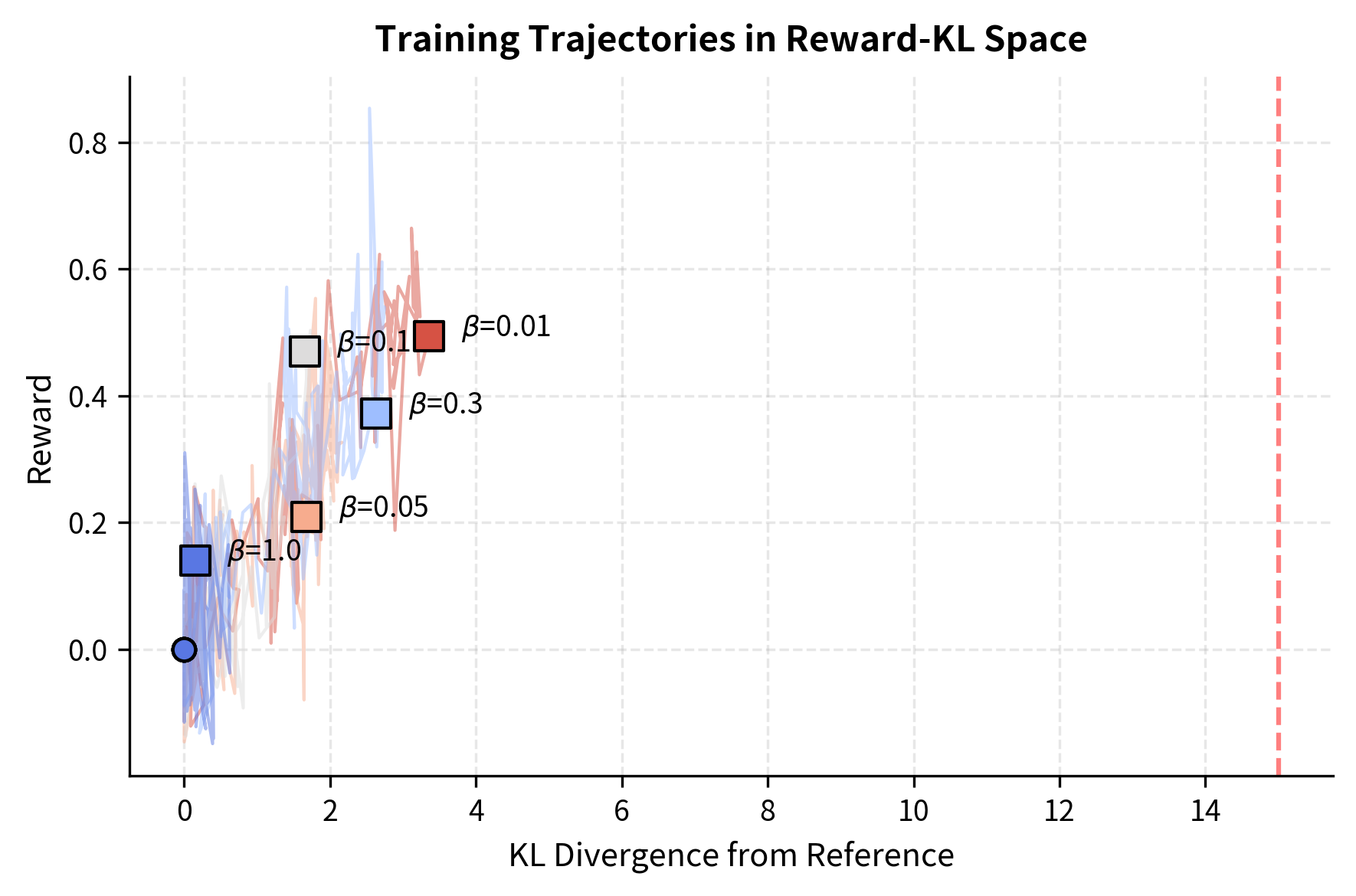
The visualization illustrates the fundamental tradeoff. Low- policies (warm colors) quickly accumulate KL divergence and can reach high rewards, but risk entering regions where the reward model is unreliable. High- policies (cool colors) progress slowly but stay in well-calibrated regions.
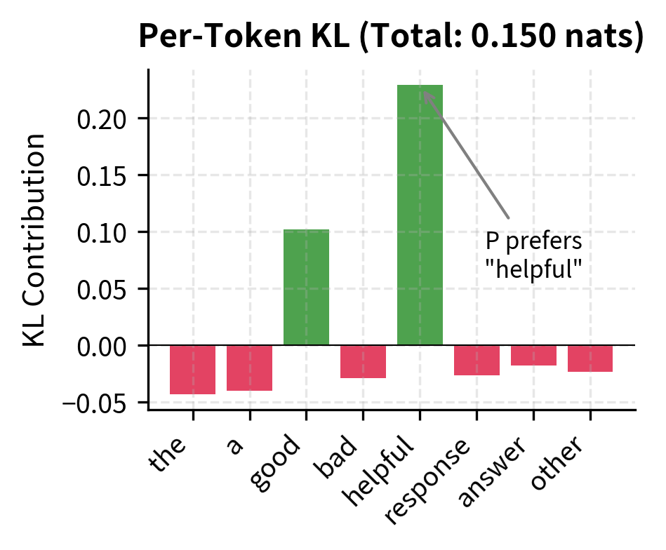
KL Distribution Over Tokens
KL divergence isn't uniform across tokens. Some positions contribute much more than others:
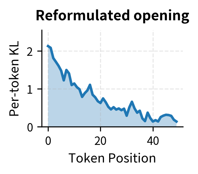
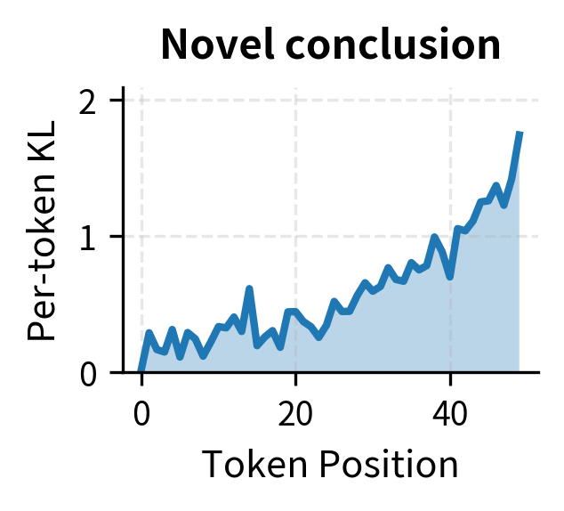
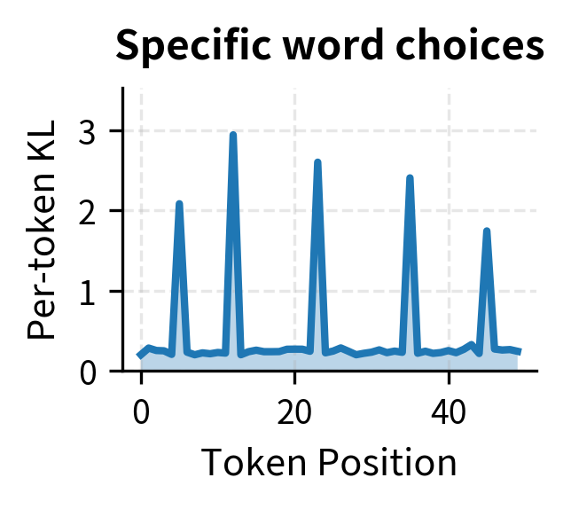
Understanding where KL accumulates helps diagnose what the policy is learning. If KL concentrates at specific positions, the policy is making targeted modifications. If KL is high throughout, the policy is developing a significantly different generation style.
Comparison: Fixed vs Adaptive KL
Let's compare training stability between fixed and adaptive KL control:
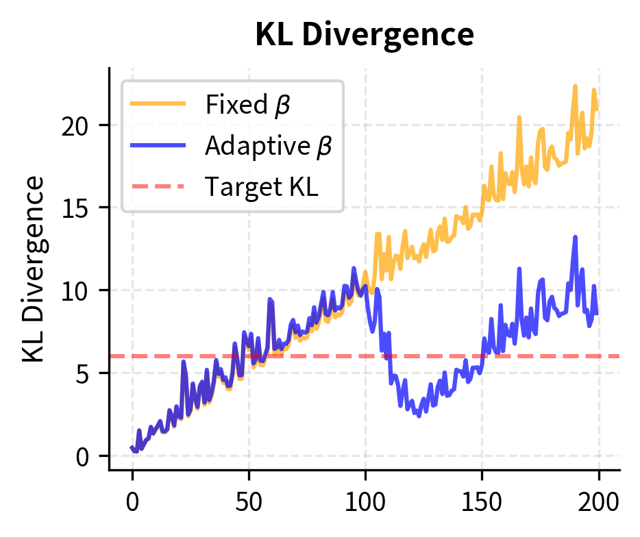
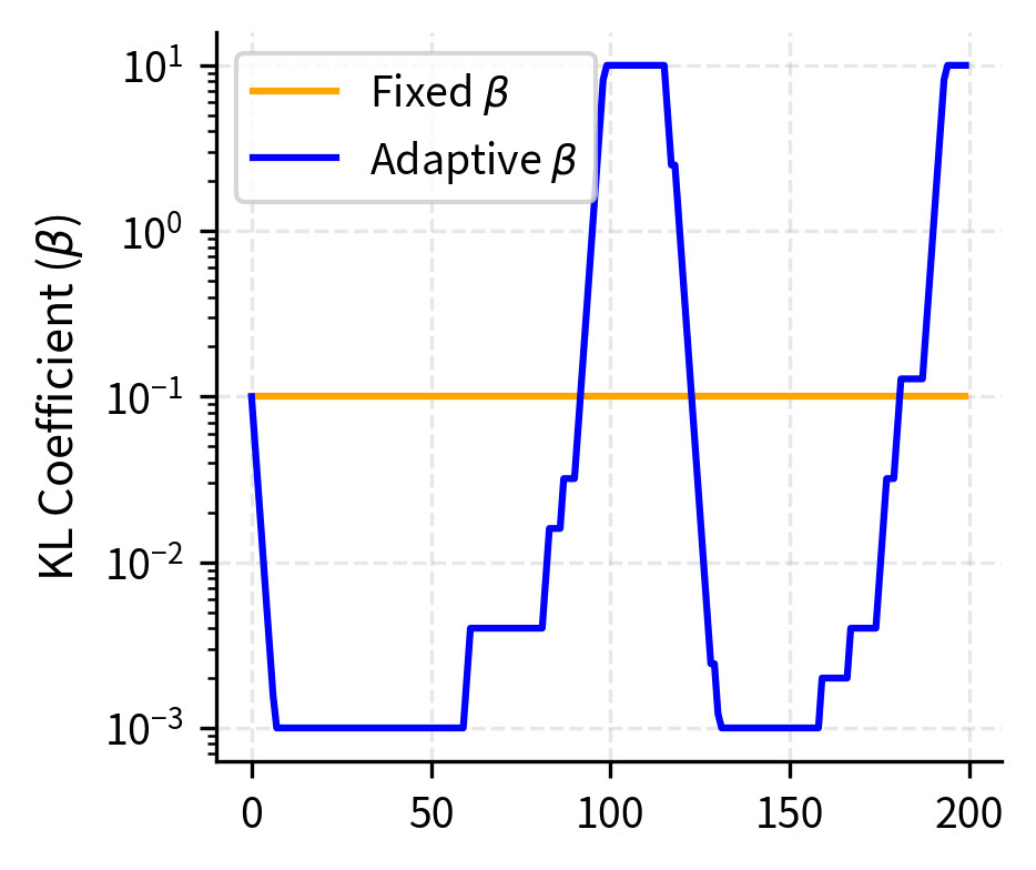
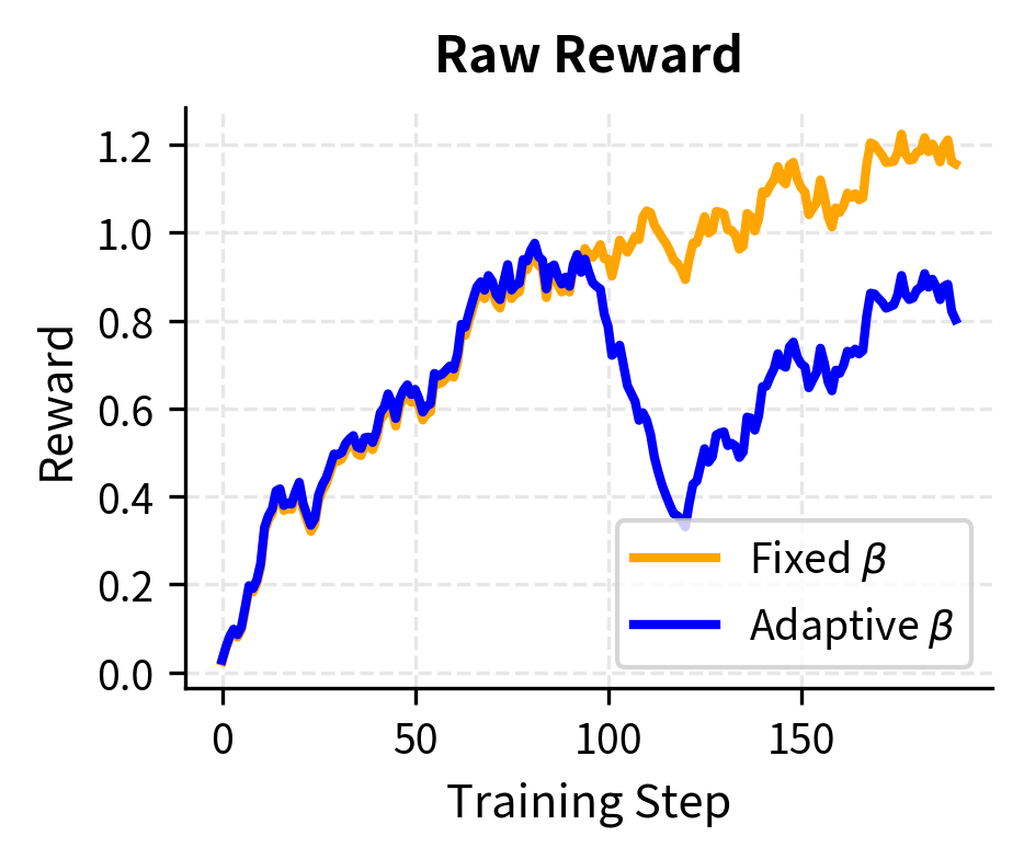
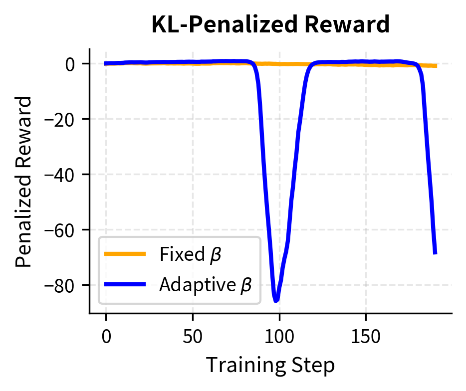
The adaptive controller maintains consistent KL divergence throughout training by increasing when the policy drifts too far. This results in more stable penalized rewards compared to the fixed controller, where the growing KL penalty eventually dominates the objective.
Limitations and Practical Considerations
While KL divergence is the standard constraint for RLHF, it has several limitations worth understanding.
Choice of reference model matters: The KL penalty anchors the policy to a specific reference, typically the SFT model. If the SFT model has problematic behaviors, the KL penalty resists correcting them. Conversely, if the SFT model is highly capable, the constraint preserves that capability. This makes the quality of supervised fine-tuning crucial for RLHF success.
KL is a distributional constraint, not a behavioral one: KL divergence measures similarity between probability distributions, not between actual behaviors. Two policies could have small KL divergence but generate quite different outputs when sampled, especially for long sequences where small per-token differences compound. Conversely, policies with large KL might produce similar outputs if the probability differences are in low-probability regions.
Asymmetry creates specific biases: The KL divergence penalizes the policy more heavily for assigning low probability to tokens the reference model assigns high probability to. This means the policy is discouraged from becoming more deterministic than the reference, which can be desirable (maintaining diversity) or undesirable (preventing confident correct answers).
Computational overhead: Computing KL requires running both the policy and reference model on every training example. For large models, this roughly doubles the forward pass compute. Some implementations amortize this by caching reference model log probabilities, but this requires additional memory.
Looking ahead, methods like Direct Preference Optimization (DPO), covered in the next chapter, incorporate the KL constraint implicitly in their objective. This eliminates the need for explicit KL computation during training while achieving similar regularization effects, representing an elegant alternative to the explicit penalty approach we've examined here.
Summary
The KL divergence penalty is essential for stable RLHF training. It prevents reward hacking by keeping the policy close to a trusted reference model, preserving the language capabilities acquired during pre-training while allowing targeted improvements in alignment.
Key takeaways from this chapter:
-
KL divergence measures distribution difference: For autoregressive models, it decomposes into a sum of per-token log probability ratios, enabling efficient computation along sampled trajectories.
-
The coefficient β controls the reward-constraint tradeoff: Low β allows rapid learning but risks exploitation of reward model errors. High β maintains stability but slows improvement. Typical values range from 0.01 to 0.2.
-
Adaptive KL control maintains consistent constraints: By adjusting β to target a specific KL budget, adaptive methods provide stable training dynamics throughout optimization, preventing both early-training instability and late-training stagnation.
-
Per-token KL reveals what the policy learns: Analyzing where KL accumulates in generated sequences helps diagnose whether the policy is making targeted modifications or developing a fundamentally different generation style.
The KL penalty represents one approach to constraining policy optimization. As we'll see in the following chapters on DPO, there are alternative formulations that achieve similar goals through different mechanisms, offering tradeoffs in implementation complexity, computational efficiency, and training stability.
Quiz
Ready to test your understanding? Take this quick quiz to reinforce what you've learned about KL divergence penalties in RLHF.

Comments