

Master the complete RLHF pipeline with three stages: Supervised Fine-Tuning, Reward Model training, and PPO optimization. Learn debugging techniques.

This article is part of the free-to-read Language AI Handbook
Choose your expertise level to adjust how many terms are explained. Beginners see more tooltips, experts see fewer to maintain reading flow. Hover over underlined terms for instant definitions.
RLHF Pipeline
Reinforcement Learning from Human Feedback transforms a base language model into an assistant that follows instructions helpfully, honestly, and safely. The previous chapters introduced the individual components: the Bradley-Terry model for preference modeling, reward model architecture and training, and the PPO algorithm adapted for language models. Now we assemble these pieces into a complete training pipeline.
The RLHF pipeline consists of three sequential stages: Supervised Fine-Tuning (SFT), Reward Model (RM) training, and PPO optimization. Each stage builds on the previous one, progressively shaping the model's behavior. This chapter walks through the complete pipeline, examining the design decisions at each stage, the hyperparameters that govern training stability, and the debugging techniques essential for successful alignment.
The Three-Stage Pipeline
The RLHF pipeline follows a specific sequence that transforms a pretrained language model into an aligned assistant. Understanding why each stage exists and how they connect is crucial for successful implementation.
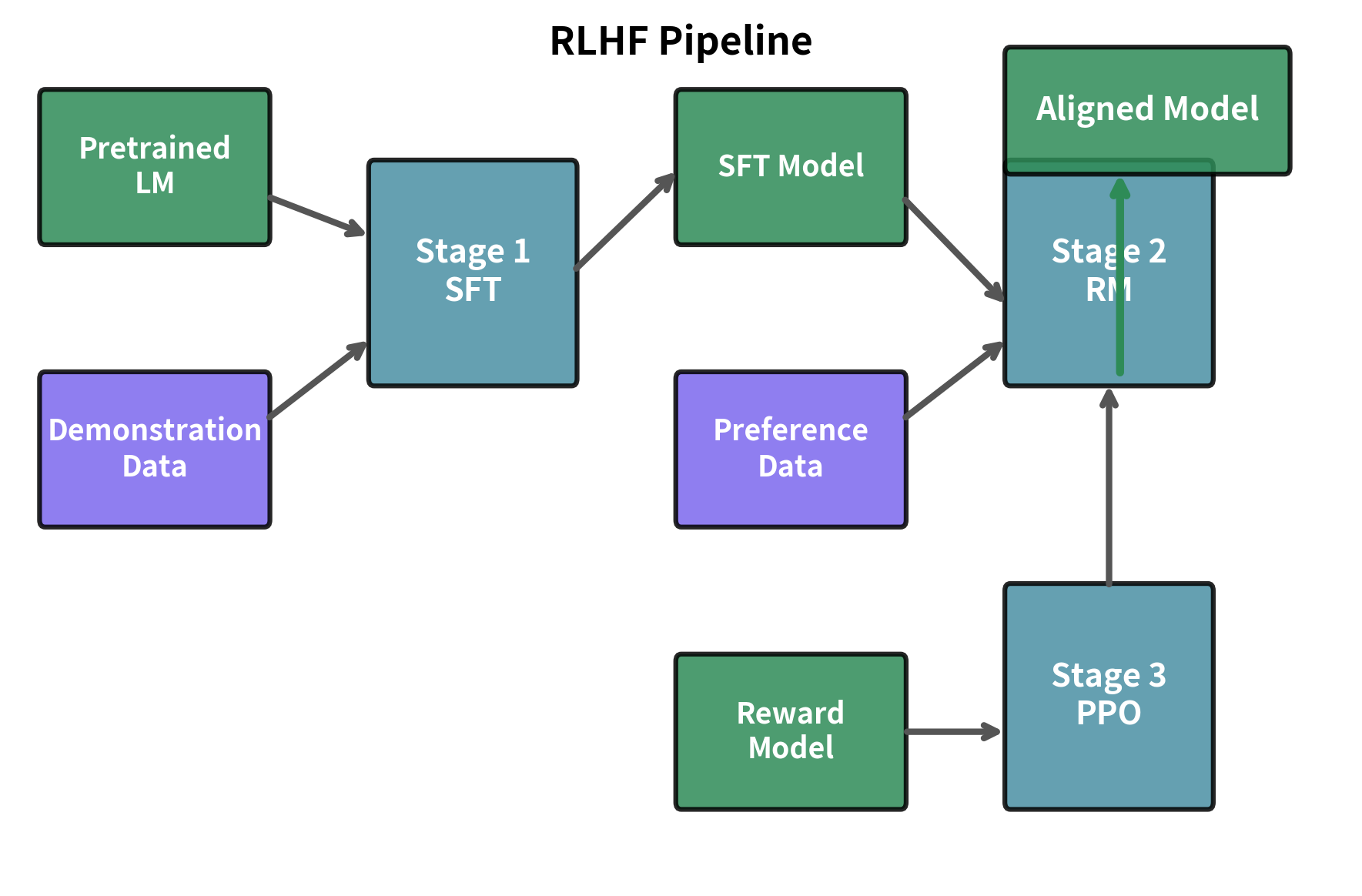
Stage 1: Supervised Fine-Tuning (SFT) takes a pretrained language model and trains it on high-quality demonstrations of desired behavior. This stage teaches the model the format and style of helpful responses, creating a starting point that can already follow instructions reasonably well.
Stage 2: Reward Model Training creates a model that predicts human preferences. Using comparison data where humans ranked alternative responses, the reward model learns to assign scalar scores reflecting response quality. As we covered in the Reward Modeling chapter, this model provides the optimization signal for the final stage.
Stage 3: PPO Fine-Tuning optimizes the SFT model to maximize rewards from the reward model while staying close to its original behavior. Building on the PPO for Language Models chapter, this stage performs the actual alignment through reinforcement learning.
Stage 1: Supervised Fine-Tuning
Supervised Fine-Tuning transforms a pretrained language model into one capable of following instructions and engaging in dialogue. While the pretrained model has acquired extensive knowledge and language understanding, it lacks the ability to respond helpfully to your queries in a conversational format.
Why SFT Comes First
You might wonder why we don't skip directly to reinforcement learning. The reason is practical: PPO optimization requires a model that already produces reasonable responses. Trying to optimize a raw pretrained model with RL is like trying to teach someone chess strategy before they know how the pieces move.
The pretrained model generates plausible continuations of text, but it doesn't understand the assistant paradigm. Given a question, it might generate more questions, continue with a different topic, or produce text that reads like training data rather than a helpful response. SFT provides the foundation by:
- Teaching the instruction-following format (recognizing prompts, generating responses)
- Establishing a baseline quality level that RL can refine
- Reducing the search space for PPO (responses are already in a useful format)
SFT Data Requirements
SFT data consists of (prompt, response) pairs demonstrating ideal assistant behavior. Quality matters far more than quantity. A few thousand high-quality demonstrations often outperform millions of lower-quality examples.
The demonstrations should exhibit properties you want the final model to have: helpfulness, appropriate tone, factual accuracy, and safety awareness. As discussed in the Instruction Data Creation chapter, these examples can come from human writers, filtered model outputs, or synthetic generation with quality controls.
SFT Training Process
SFT uses standard causal language modeling loss but only on the response tokens. This distinction is crucial for understanding how the model learns during this stage. The prompt provides context, allowing the model to understand what kind of response is expected, but we don't penalize the model for not predicting prompt tokens. The reasoning is straightforward: we only want the model to learn how to respond given a prompt, not to memorize and reproduce the prompts themselves.
The training objective focuses exclusively on maximizing the likelihood of generating the correct response tokens, conditioned on the full context of the prompt. This targeted learning ensures the model develops the skill of producing appropriate responses rather than simply learning to continue arbitrary text.
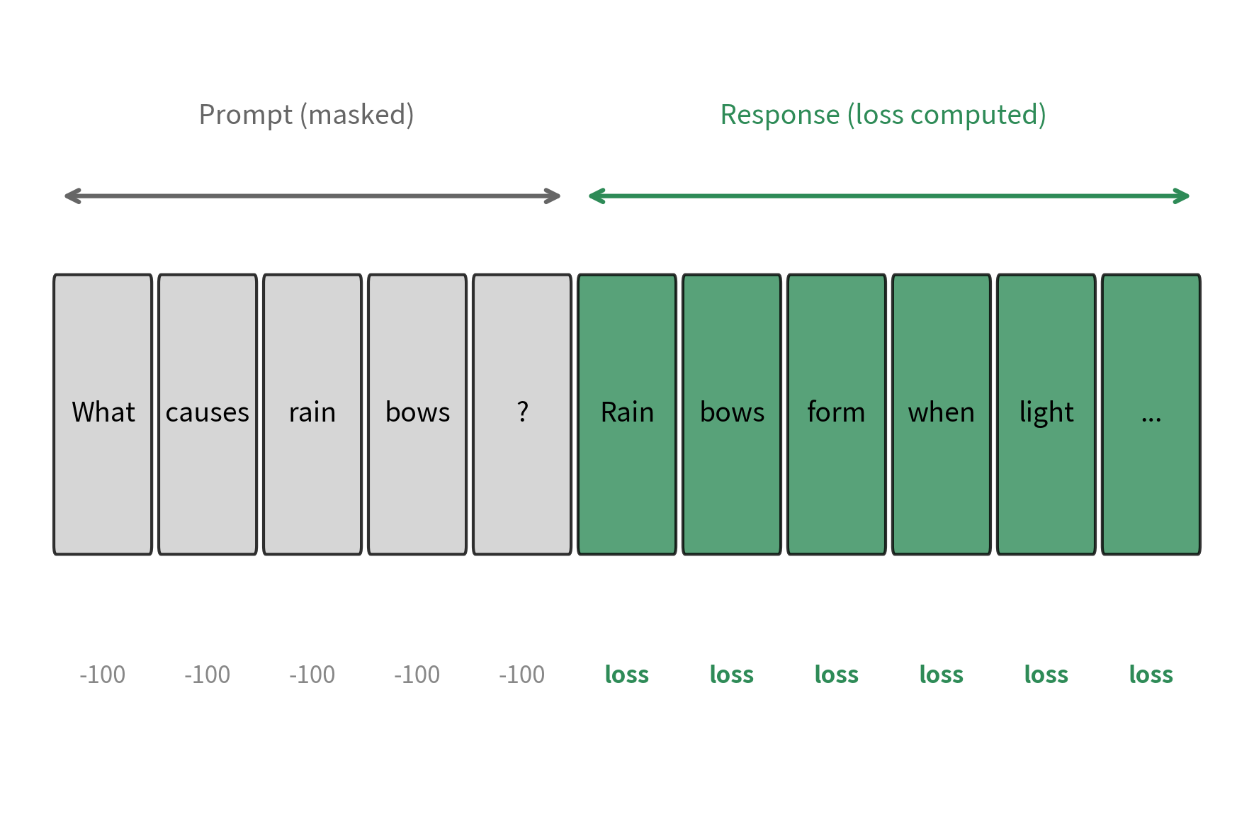
The key detail is setting labels to -100 for prompt tokens. This value serves as a special sentinel in PyTorch's CrossEntropyLoss function: any token position with a label of -100 is completely ignored during loss computation. By masking the prompt tokens this way, we ensure we only compute loss on the response portion, teaching the model to generate good responses without wasting gradient updates on predicting prompt content it doesn't need to reproduce.
Key Parameters
SFT training is relatively straightforward compared to the later stages. The key parameters are:
- Learning rate: Typically 1e-5 to 5e-5 for full fine-tuning, or 1e-4 to 3e-4 for LoRA (as covered in the LoRA chapters)
- Batch size: 32 to 128 examples, depending on available memory
- Epochs: 1-3 passes over the data; more risks overfitting
- Warmup: 3-10% of total steps with linear warmup
Overfitting is a real concern with small SFT datasets. Monitor validation loss and stop training when it begins to increase. You might prefer training for slightly fewer steps than optimal to preserve model generalization.
Stage 2: Reward Model Training
The reward model learns to predict which responses humans prefer. Building on the Bradley-Terry model from earlier chapters, it converts pairwise comparisons into a scalar reward signal that guides PPO optimization.
Reward Model Architecture
As discussed in the Reward Modeling chapter, the reward model typically shares architecture with the language model but replaces the language modeling head with a scalar output head. This architectural choice is deliberate: by starting from a language model that understands text, the reward model inherits the ability to comprehend nuanced language, context, and meaning. The only modification is the final layer, which now outputs a single number representing quality rather than a distribution over vocabulary tokens.
The reward model extracts the hidden state at the final token position and passes it through a small neural network to produce a scalar reward. This design leverages an important property of causal transformers: the final token's hidden state has attended to all previous tokens in the sequence, meaning it encapsulates information about the entire prompt-response pair. By using this aggregated representation, the model can make a holistic quality judgment that considers both what was asked and how well the response addresses it.
Preference Data Format
Training data consists of prompts with two or more responses ranked by human annotators. Each training example captures a comparison: given the same prompt, which response did humans consider better? This pairwise structure is fundamental to the Bradley-Terry model, which we'll examine shortly.
The training examples typically show that chosen responses are longer, more detailed, and better structured than rejected ones. The reward model learns to associate these features, along with factual accuracy and tone, with higher scalar scores.
Reward Model Training Loss
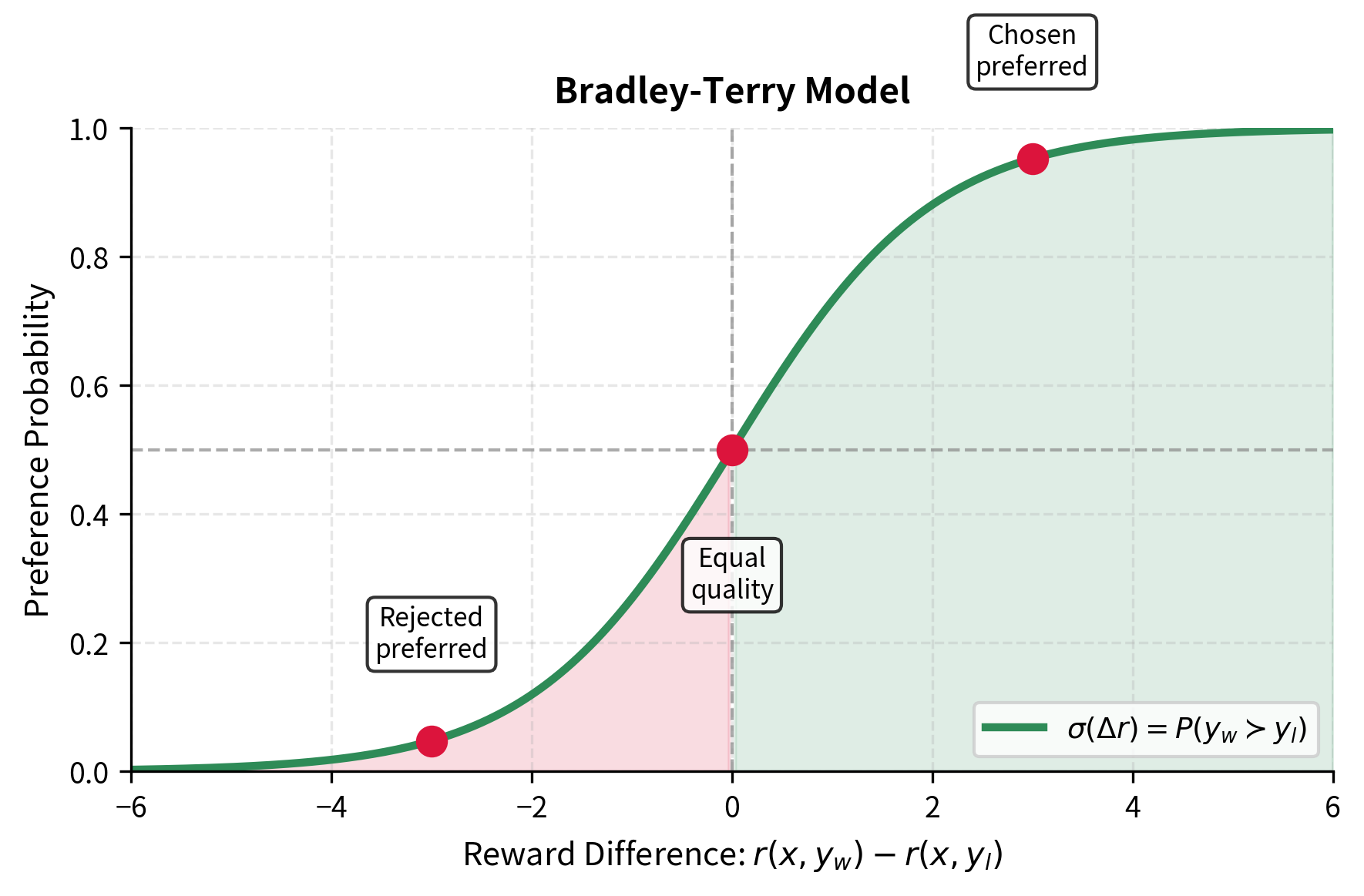
The training objective for the reward model emerges from a probabilistic framework for modeling human preferences. We begin with a natural question: given two responses to the same prompt, how likely is it that a human prefers one over the other? The Bradley-Terry model provides an elegant answer by relating this preference probability to the difference in quality scores assigned to each response.
The core insight is that we can model preferences as arising from latent quality scores. If response has a higher quality score than response , then should be preferred more often. The Bradley-Terry model formalizes this intuition by expressing the preference probability as a function of the score difference:
where:
- : the probability that response is preferred over given prompt
- : the logistic sigmoid function,
- : the reward model with parameters
- : the input prompt
- : the preferred ("winning") response
- : the rejected ("losing") response
The sigmoid function plays a crucial role in this formulation. It converts the unbounded difference in reward scores into a probability between 0 and 1, providing a smooth and differentiable mapping. When the reward for the winning response is significantly larger than for the losing response, the difference becomes a large positive number, and the sigmoid approaches 1, indicating near-certainty that would be preferred. Conversely, if the scores are equal, the sigmoid returns 0.5, reflecting maximum uncertainty. This elegant mathematical structure captures our intuition that larger quality differences should correspond to more decisive preferences.
To train the model, we minimize the negative log-likelihood of observing the preferences in our dataset. For a single preference pair, the loss is:
where:
- : the scalar loss value to be minimized
- : the logistic sigmoid function,
- : the reward model with parameters that assigns a scalar score to a prompt-response pair
- : the input prompt or instruction
- : the "winning" or preferred response
- : the "losing" or rejected response
- : the difference in reward scores (which we want to be positive)
Understanding why this loss works requires examining what happens during optimization. When the model correctly assigns a higher score to the preferred response (making the difference positive and large), the sigmoid outputs a value close to 1, and the negative log becomes small. When the model incorrectly ranks the responses (making the difference negative), the sigmoid outputs a value close to 0, and the negative log becomes very large, creating a strong gradient signal to correct this error. This objective therefore directly maximizes the likelihood that the model assigns a higher score to the preferred response than the rejected response , which is precisely what we want from a reward model.
Reward Model Training Metrics:
- Loss: Bradley-Terry negative log-likelihood
- Accuracy: Fraction where
- Target accuracy: 70-80% (higher may indicate overfitting)
Reward Model Calibration
A critical but often overlooked aspect is reward model calibration. The absolute reward values don't matter for ranking, since the Bradley-Terry model only uses differences between scores. However, the scale of these values significantly affects PPO training stability. If rewards are too large in magnitude, gradient updates can become unstable; if they vary too widely, the optimization landscape becomes difficult to navigate.
Stage 3: PPO Fine-Tuning
With the SFT model and reward model ready, we can now run PPO optimization. This stage adjusts the policy to maximize expected reward while staying close to the SFT model's behavior. The challenge here is delicate: we want the model to improve according to the reward signal without losing the coherent language abilities it acquired during pretraining and SFT.
The PPO Training Loop
As we detailed in the PPO for Language Models chapter, each training iteration involves a carefully orchestrated sequence of steps that together enable stable policy improvement:
- Sampling: Generate responses from the current policy
- Reward computation: Score responses using the reward model
- Advantage estimation: Compute advantages using GAE
- Policy update: Optimize the clipped surrogate objective. This iterative process gradually shifts the policy's behavior toward responses that score higher according to the reward model, while the various stability mechanisms in PPO prevent the optimization from taking steps that are too large or in harmful directions.
Computing the Complete Reward
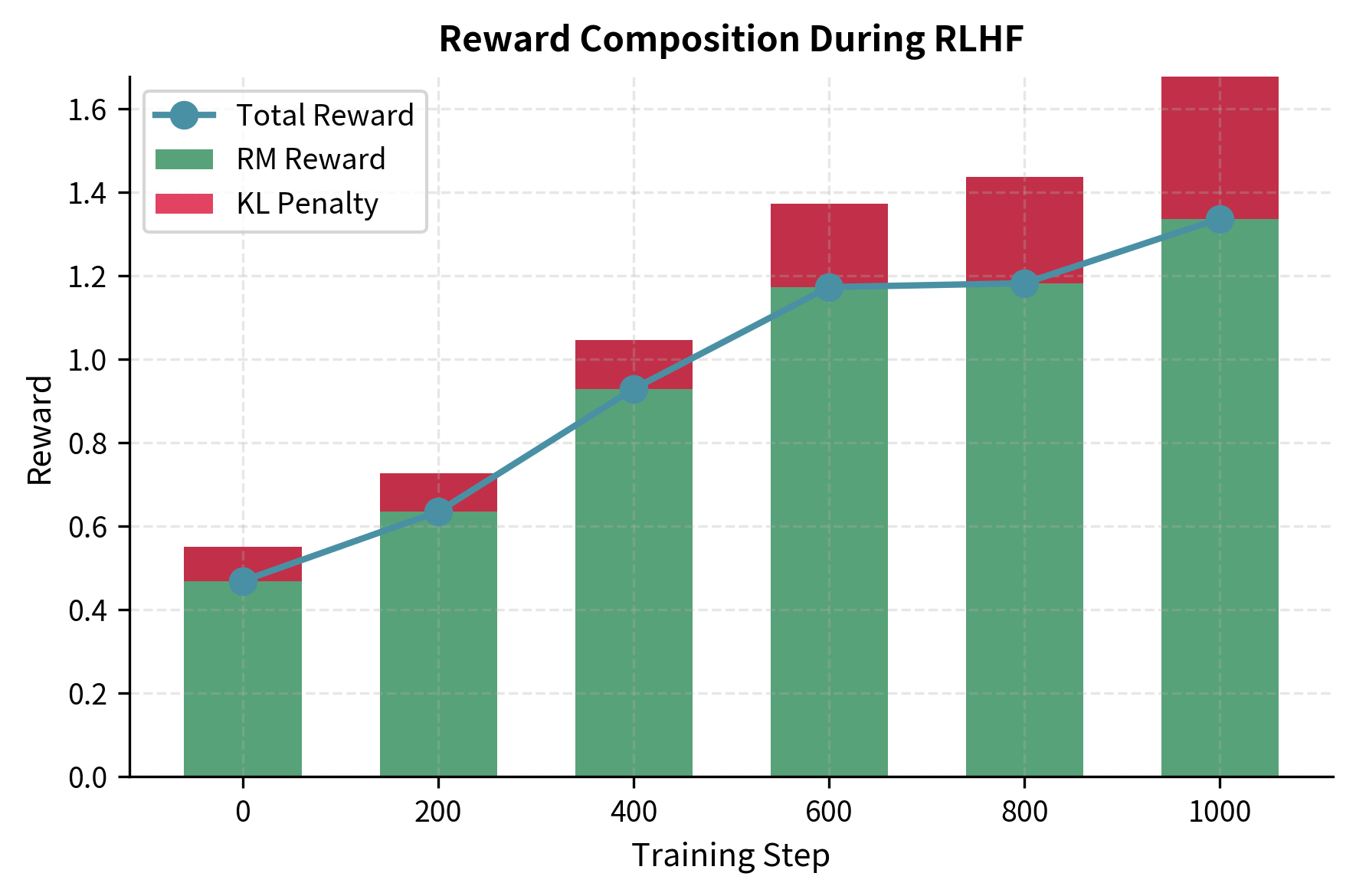
The total reward used to update the policy combines two competing objectives. We want to maximize the reward model's score, which represents human preferences, but we also want to prevent the policy from straying too far from the reference model, which represents stable, coherent language generation. The KL divergence penalty provides this regularization, creating a tug-of-war that encourages improvement without catastrophic drift.
We'll explore the KL divergence penalty in detail in the next chapter, but the basic formulation captures this balance mathematically:
where:
- : the combined reward used to update the policy
- : the input prompt
- : the generated response
- : the preference score from the reward model
- : the KL penalty coefficient controlling regularization strength
- : the Kullback-Leibler divergence between the two distributions
- : the current policy model
- : the reference model (frozen SFT model)
The KL coefficient acts as a dial controlling the trade-off between reward maximization and behavioral stability. A larger keeps the policy closer to the reference model, preserving more of the original capabilities but potentially limiting how much the model can improve. A smaller allows more aggressive optimization toward higher rewards, but risks the policy finding reward model exploits or losing coherence. This formulation ensures that while we maximize the preference score, we maintain the linguistic coherence and knowledge of the original model.
PPO Update Step
The policy update uses the clipped surrogate objective from the PPO Algorithm chapter. This objective function represents the core mechanism that enables stable policy improvement: rather than directly maximizing expected reward, which could lead to catastrophically large updates, PPO constrains how much the policy can change in a single step. The clipping mechanism ensures that even if the advantage estimates suggest a large improvement, the actual policy update remains bounded.
RLHF Debugging
RLHF training is notoriously difficult to debug. The interplay between the policy, reward model, and KL constraint creates many potential failure modes.
Key Metrics to Monitor
Effective RLHF debugging requires tracking multiple metrics throughout training:
The metrics tracker successfully identifies the simulated anomalies. By monitoring the KL divergence and reward statistics we can catch issues like the "High KL" spike and "High Reward" events (simulating reward hacking) before they destabilize the entire training run.
### Common Failure Modes
Understanding these failure modes helps you diagnose and fix training issues:
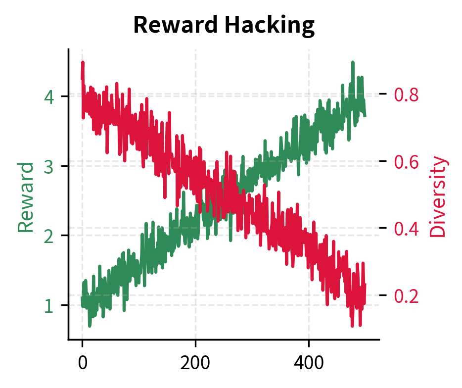
Reward Hacking occurs when the policy finds exploits in the reward model that don't correspond to genuine quality improvements. Signs include rapidly increasing reward with degrading response quality, or unusual patterns like excessive repetition or specific phrases.
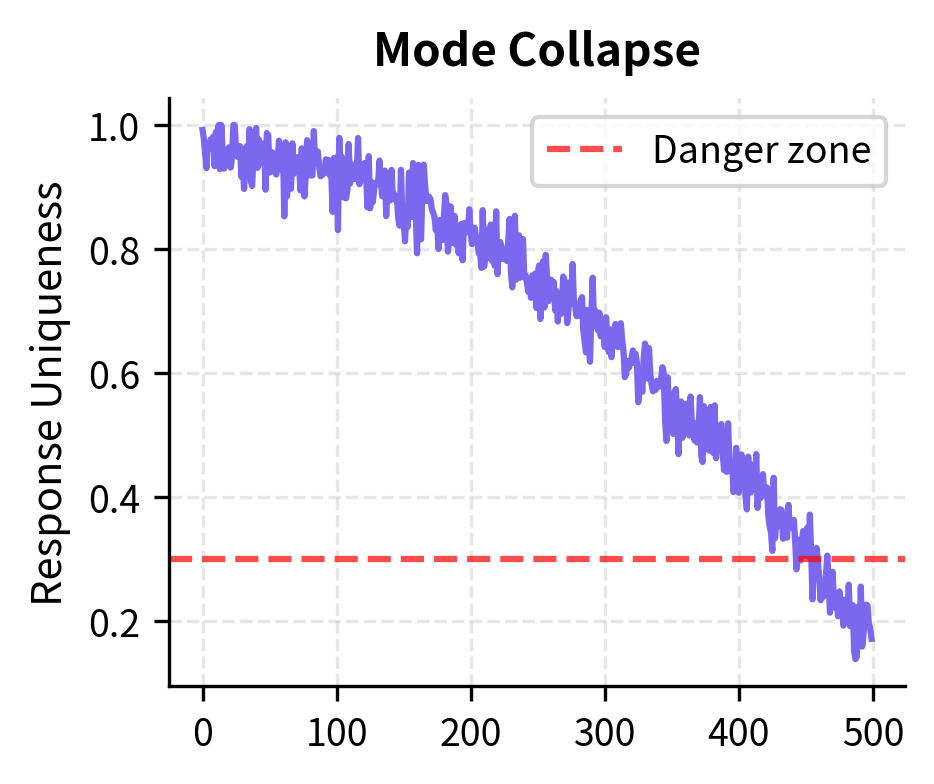
Mode Collapse happens when the policy converges to producing nearly identical responses regardless of the prompt. Monitor response diversity and entropy throughout training.
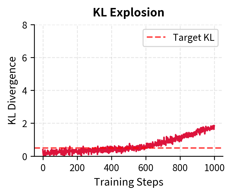
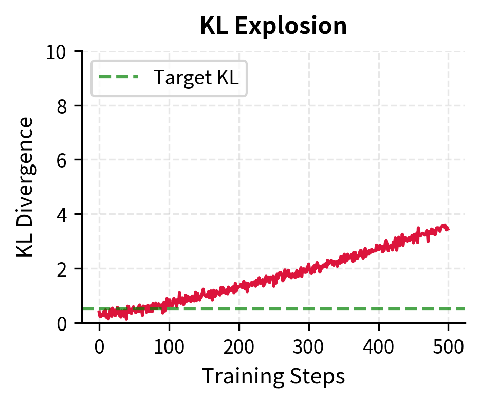
KL Explosion indicates the policy is moving too fast away from the reference model. This often precedes training instability:
Debugging Workflow
When RLHF training goes wrong, follow this systematic debugging approach:
-
Check the reward model first: Generate samples and manually verify that reward model scores align with your quality intuitions. A miscalibrated or overfitted reward model dooms PPO from the start.
-
Examine generated samples: Look at actual model outputs throughout training. Metrics can hide problems that become obvious when reading responses.
-
Verify the KL penalty is working: The policy should stay reasonably close to the reference. If responses look completely different from SFT outputs, the KL constraint may be too weak.
-
Monitor multiple metrics together: Single metrics can be misleading. High reward with low diversity suggests reward hacking. Low KL with no reward improvement suggests the policy isn't learning.
Putting It All Together
Let's trace through a complete RLHF training run, showing how all pieces connect:
The text output confirms that each stage completed successfully. The SFT loss decreased significantly, and the Reward Model achieved a validation accuracy of 74%, which is within the typical 70-80% range for effective preference modeling. These healthy prerequisites set the stage for the PPO phase, which we can now visualize.
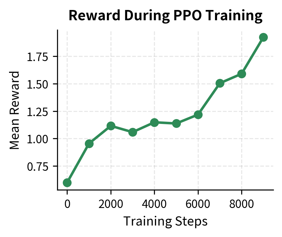
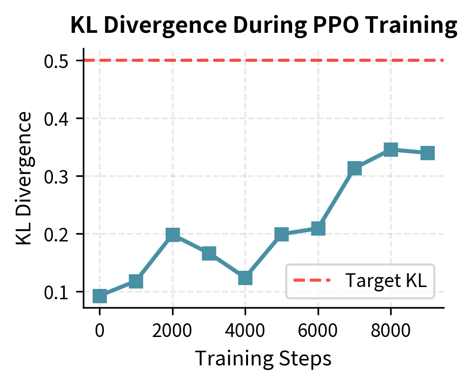
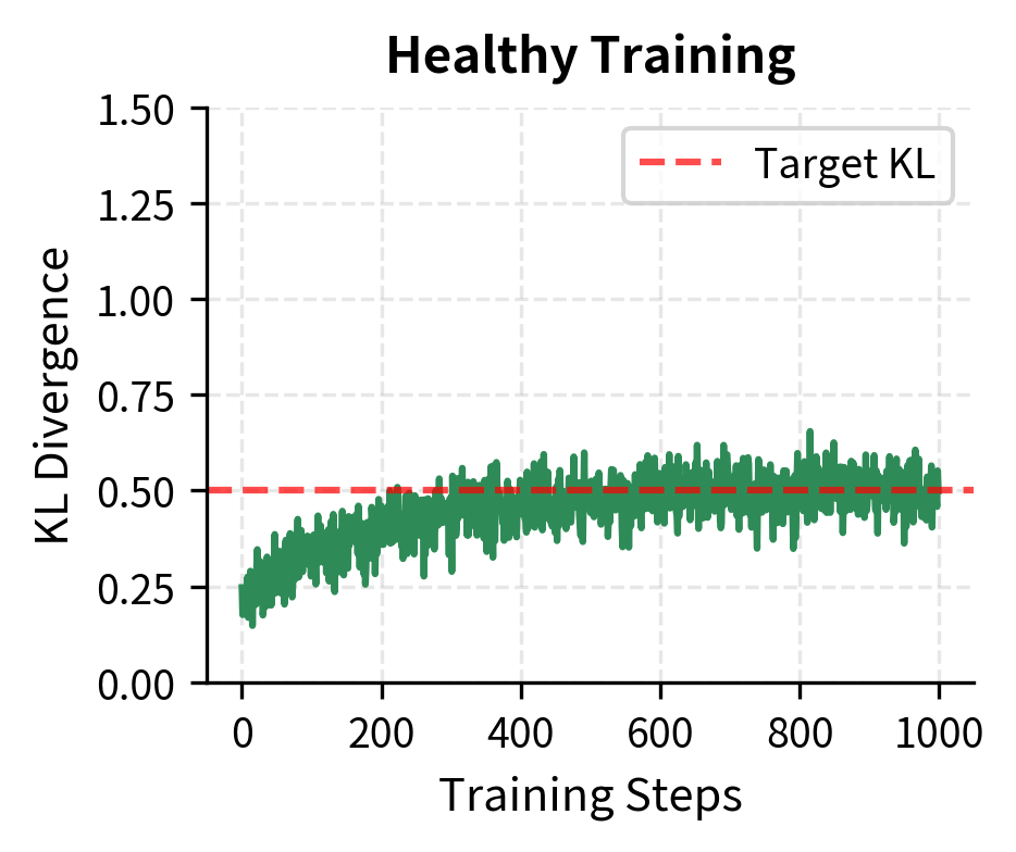
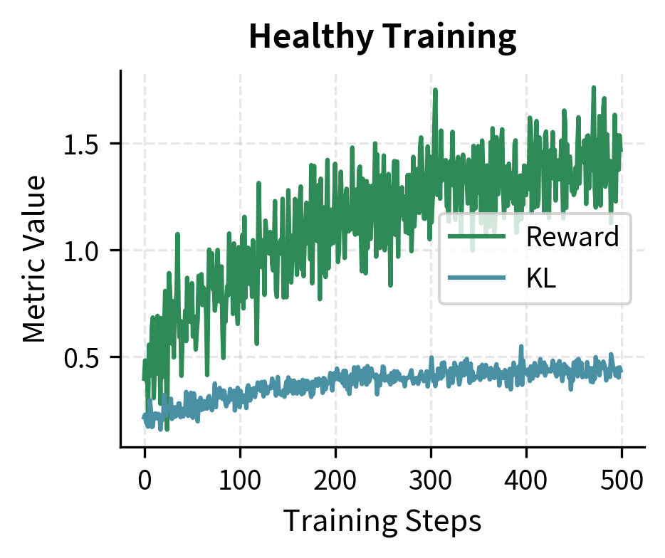
The training curves demonstrate healthy alignment progress. The reward (left) steadily increases, indicating the model is learning to satisfy the reward model's preferences. Meanwhile, the KL divergence (right) remains controlled near the target of 0.5, ensuring the model maintains the coherent capabilities of the original SFT model without drifting into incoherence or reward hacking.
Limitations and Practical Considerations
The RLHF pipeline, while powerful, comes with significant challenges that you must navigate.
Computational cost is substantial. The pipeline requires training three separate models (SFT, reward model, and PPO policy), with the PPO stage being particularly expensive because it requires running both the policy and reference model for every batch. A single RLHF training run can cost hundreds of thousands of dollars in compute for large models, making iteration and experimentation prohibitively expensive for most organizations. This has driven interest in more efficient alternatives like Direct Preference Optimization (DPO), which we'll explore in upcoming chapters.
Human annotation quality fundamentally limits what RLHF can achieve. The reward model can only capture patterns present in the preference data, and human annotators bring their own biases, inconsistencies, and limitations. Disagreement between annotators is common, yet the Bradley-Terry model assumes a consistent underlying preference ordering. When annotators disagree about what makes a response "better," the reward model learns a noisy compromise that may not align with your preferences.
Reward hacking remains an unsolved problem despite various mitigation strategies. As we discussed in the Reward Hacking chapter, the policy will exploit any systematic weakness in the reward model. The KL penalty helps by anchoring behavior to the reference model, but sufficiently capable policies can still find exploits within the allowed KL budget. This creates an ongoing cat-and-mouse dynamic where you must continually patch reward model vulnerabilities.
Reproducibility is challenging due to the many interacting hyperparameters and the sensitivity of PPO training. Small changes in learning rate, KL coefficient, or even random seed can lead to qualitatively different outcomes. This makes it difficult to compare results across papers or replicate published findings.
Despite these limitations, RLHF remains the most widely deployed alignment technique for production language models. Understanding the complete pipeline, including its failure modes, is essential for anyone working on language model alignment. The next chapter examines the KL divergence penalty in detail, which plays a crucial role in balancing reward maximization with behavioral stability.
Summary
The RLHF pipeline transforms a pretrained language model into an aligned assistant through three sequential stages. Supervised Fine-Tuning creates a model that understands the instruction-following format and produces reasonable responses. Reward Model training captures human preferences in a learnable function that provides optimization signal. PPO Fine-Tuning then optimizes the policy to maximize rewards while staying close to the reference model.
Key takeaways from this chapter:
- SFT provides the foundation: PPO requires a model that already produces usable responses; skipping SFT leads to unstable training
- Reward model quality is paramount: A flawed reward model will lead to flawed policies; validate carefully before PPO
- KL penalty prevents catastrophic drift: Without anchoring to the reference model, the policy will exploit reward model weaknesses
- Monitor multiple metrics: Single metrics can be misleading; track reward, KL, entropy, and response characteristics together
- Debugging requires examining actual outputs: Metrics summarize behavior, but reading generated responses reveals problems that numbers hide
The RLHF pipeline established the template for aligning large language models, but its complexity and cost have motivated simpler alternatives. The next chapter examines the KL divergence penalty in mathematical detail, followed by chapters on Direct Preference Optimization, which eliminates the reward model and PPO stages entirely while achieving comparable alignment results.
Quiz
Ready to test your understanding? Take this quick quiz to reinforce what you've learned about the RLHF pipeline.

Comments