

Learn antithetic variates, control variates, and stratified sampling to reduce Monte Carlo simulation variance by 10x or more for derivatives pricing.
Choose your expertise level to adjust how many terms are explained. Beginners see more tooltips, experts see fewer to maintain reading flow. Hover over underlined terms for instant definitions.
Variance Reduction Techniques in Simulation
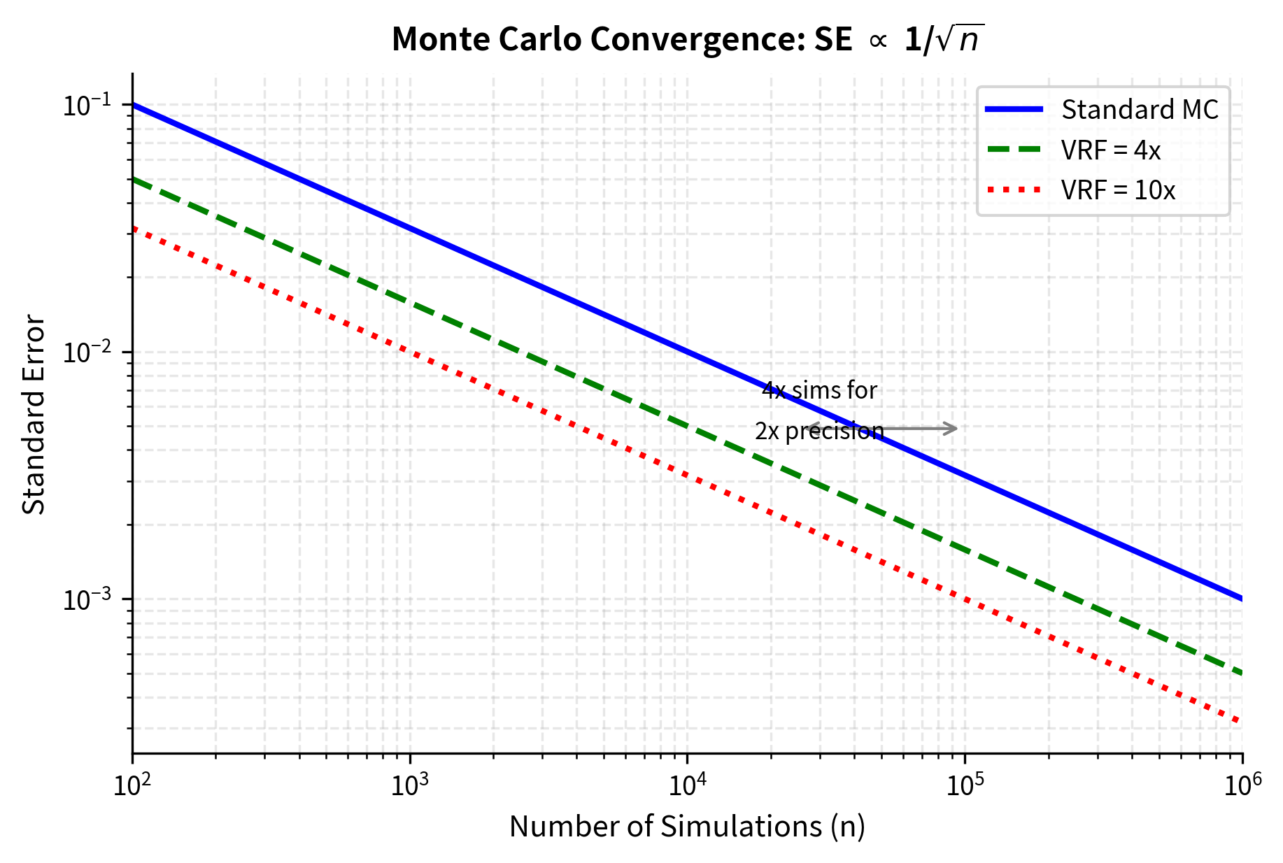
In the previous chapter, we explored Monte Carlo simulation as a powerful method for pricing derivatives that lack closed-form solutions. The technique's elegance lies in its simplicity: simulate many paths of the underlying asset, compute the payoff for each path, and average the discounted results. However, simplicity comes at a computational cost. To achieve accurate prices, we often need millions of simulations, and the standard error decreases only as , where is the number of simulations. This means reducing the error by half requires four times as many simulations.
For complex derivatives, path-dependent options, or real-time risk calculations, this computational burden becomes prohibitive. Variance reduction techniques address this challenge by modifying the simulation procedure to produce estimates with lower variance for the same number of simulations, or equivalently, achieving the same accuracy with far fewer simulations. These techniques exploit mathematical structure in the problem, such as symmetry, known analytical results, or strategic sampling, to squeeze more information from each simulation.
This chapter introduces three foundational variance reduction methods: antithetic variates, control variates, and stratified sampling. Each technique attacks the variance problem from a different angle. Understanding when to apply each method is crucial for efficient derivative pricing. By the end of this chapter, you will be able to reduce simulation time by factors of 10 or more without sacrificing accuracy, a capability that separates practical quantitative work from textbook exercises.
The Variance Problem in Monte Carlo Estimation
Let's precisely characterize the problem we're solving. The core challenge of Monte Carlo simulation stems from the inherent randomness of the sampling process itself. Every time we run a simulation, we draw random samples from a probability distribution, and these samples inevitably fluctuate around the true expected value. Understanding the mathematical structure of this fluctuation reveals both the limitation of brute-force approaches and the opportunities for variance reduction.
Recall from our work on Monte Carlo simulation that we estimate an expectation using the sample mean:
where:
- : the sample mean estimator
- : number of simulations
- : independent samples from the distribution of
This estimator forms the foundation of all Monte Carlo methods. By the law of large numbers, as we increase the number of samples , the sample mean converges to the true expected value . This convergence guarantees that our estimates become increasingly accurate with more simulations. However, the central limit theorem tells us precisely how fast this convergence occurs, and understanding this rate is essential for appreciating both the challenge and the solution.
The variance of this estimator is:
where:
- : variance of the estimator
- : variance of a single sample,
- : number of simulations
This formula deserves careful attention because it encapsulates the entire variance reduction problem. Notice that the numerator, , represents the intrinsic variability of individual samples. This is the randomness inherent in the payoff of each simulated path. The denominator, , represents our computational effort. The ratio tells us that the precision of our estimate depends on both how variable our individual samples are and how many samples we collect.
The standard error, which measures the typical distance between our estimate and the true value, is:
where:
- : standard error of the estimator
- : standard deviation of a single sample
- : number of simulations
The square root in the denominator is the source of Monte Carlo's computational challenge. This equation reveals two fundamentally different ways to reduce estimation error, and understanding the distinction between them illuminates the entire field of variance reduction.
The first approach is to increase , the number of simulations. This is the brute force method, but the in the denominator means diminishing returns: reducing error by a factor of 10 requires 100 times more simulations. To appreciate how severe this limitation is, consider that reducing error from 1% to 0.1% requires increasing simulations from, say, 10,000 to 1,000,000. This hundredfold increase in computational cost makes brute-force approaches impractical for many applications, particularly when each simulation involves complex path-dependent calculations.
The second approach is to reduce , the variance of individual samples. This is the variance reduction approach. If we can modify our simulation procedure to produce samples with lower variance while maintaining the same expected value, we achieve more accurate estimates without additional computational cost. This insight is the key to everything that follows in this chapter. Rather than fighting against the convergence rate by throwing more computation at the problem, we can work smarter by reducing the numerator in the standard error formula.
The efficiency gain from variance reduction can be quantified by comparing the variance of the standard Monte Carlo estimator to the variance of the improved estimator. If the improved method has variance instead of , the variance reduction factor is:
where:
- : Variance Reduction Factor
- : variance of the single sample in standard Monte Carlo
- : equivalent single-sample variance of the improved method
This ratio provides a concrete measure of improvement. A variance reduction factor of 10 means you need only one-tenth as many simulations to achieve the same accuracy. For complex derivatives where each simulation involves hundreds of time steps and multiple correlated assets, this translates directly into substantial computational savings. Equivalently, you can think of the variance reduction factor as the effective multiplier on your computational resources: a VRF of 10 makes your computer effectively 10 times faster for this particular calculation.
The three techniques we explore in this chapter, antithetic variates, control variates, and stratified sampling each attack the variance problem from a different angle. Antithetic variates introduce negative correlation between samples, causing overestimates to cancel with underestimates. Control variates leverage known information about related quantities to adjust our estimates. Stratified sampling ensures that our random samples cover the input space more uniformly, eliminating variance caused by accidental clustering. Together, these methods form a powerful toolkit that transforms Monte Carlo simulation from a computationally expensive necessity into a practical tool for real-time pricing.
Antithetic Variates
Antithetic variates exploit a symmetry in the random sampling process to reduce variance with minimal computational overhead. This section develops the mathematical foundation and provides practical implementation guidance.
The Core Intuition
Antithetic variates exploit a simple but powerful idea: instead of generating independent random samples, we generate pairs of negatively correlated samples. The negative correlation causes high estimates from one sample to partially cancel with low estimates from its partner. This reduces overall variance. To understand why this works, consider what happens when we average two random numbers compared to averaging two numbers that move in opposite directions.
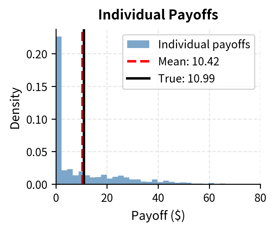
Consider estimating the expected payoff of a call option. Some simulations will produce paths where the asset price ends up high (large payoff), while others will produce paths where it ends up low (zero payoff). If we could pair each "high" outcome with a corresponding "low" outcome, the average of each pair would be closer to the true expected value than either outcome alone. This pairing creates a cancellation effect where extreme values offset each other, producing more stable estimates.
The antithetic technique implements this pairing by using the symmetry of the standard normal distribution. If is a standard normal random variable then is also standard normal with the same distribution. More importantly, and are perfectly negatively correlated. When we use to generate one path and to generate an "antithetic" path, the two paths move in opposite directions, creating the cancellation effect we seek. This symmetry property of the normal distribution is not merely a mathematical curiosity; it is a structural feature we can exploit for practical benefit.
Mathematical Foundation
To understand precisely how antithetic variates reduce variance, we need to formalize the relationship between the original and antithetic samples and analyze the resulting estimator. Let where is a standard normal random variable and is the function mapping random inputs to payoffs. Define the antithetic variable . Since has the same distribution as , we have . This ensures the antithetic sample does not bias our estimate.
The antithetic estimator uses the average of each pair:
where:
- : the antithetic estimator
- : payoff from the original sample
- : payoff from the antithetic sample
- : payoff function
- : standard normal random variable
This average forms the building block of the antithetic variates method. Rather than treating each simulation independently, we pair simulations and work with the average of each pair. The key question is whether this pairing reduces variance compared to using the same total number of independent samples.
The expected value of equals the expected value we want to estimate:
where:
- : the antithetic estimator
- : payoff from the original sample
- : payoff from the antithetic sample
- : expected value of target variable
This calculation confirms that the antithetic estimator is unbiased. The expected value of our estimate equals the true quantity we want to estimate, regardless of how and are correlated. Unbiasedness is essential because it guarantees that our estimate converges to the correct value as we increase the number of simulations.
Now we turn to the crucial analysis of variance. The variance of is:
where:
- : variance of the antithetic estimator
- : variance of the single sample
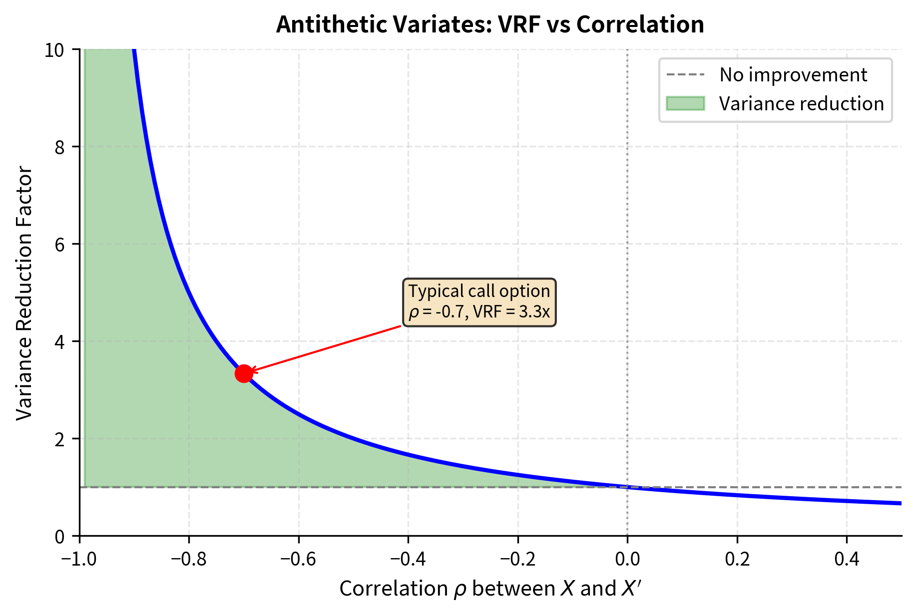
- : correlation between and ,
This variance formula reveals the mathematical heart of the antithetic variates method. The key term is , which depends on the correlation between the original and antithetic samples. When independent samples are used, , and the variance of the average of two samples would be . But when the samples are negatively correlated, meaning , the term becomes smaller than 1, reducing the variance below what independent sampling would achieve.
For variance reduction to occur, we need (since we use two samples to compute ). This requires:
where:
- : variance of the single sample
- : correlation between the antithetic pair
which simplifies to . The more negative the correlation, the greater the variance reduction. In the extreme case where , the variance of the pair average drops to zero, meaning the average of and equals the true expected value exactly. While perfect negative correlation is rarely achievable in practice, even moderate negative correlation provides substantial variance reduction.
When Antithetic Variates Work
The correlation depends on the function . For monotonic functions antithetic variates are highly effective. Consider a call option payoff, which increases with the underlying asset price. High values of lead to high terminal prices and high payoffs; low values of (or equivalently, high values of ) lead to low terminal prices and low payoffs. The payoffs from and move in opposite directions, creating strong negative correlation.
To understand this more concretely, imagine a call option with a strike price at the current asset level. When we draw a positive value of , the asset drifts upward, ending above the strike and producing a positive payoff. The antithetic sample uses , which pushes the asset downward, likely ending below the strike with zero payoff. The average of a positive payoff and zero is closer to the true expected value than either extreme would be alone. This systematic pairing of high and low outcomes is what drives the variance reduction.
::: {.callout-note title="Monotonicity Condition" Antithetic variates reduce variance when the payoff function is monotonic in the underlying random variables. For option pricing, this typically holds because option values increase (for calls) or decrease (for puts) with the underlying asset price. :::
For non-monotonic payoffs, such as straddles or butterfly spreads, the effectiveness diminishes because the payoff might increase and then decrease as the underlying moves, breaking the negative correlation. A straddle, for instance, pays off when the underlying moves far from the strike in either direction. Both and could produce large movements, just in opposite directions, so both could yield high payoffs. The pairing no longer creates the cancellation effect that drives variance reduction.
Implementation for European Options
Let's implement antithetic variates for pricing a European call option and compare it to standard Monte Carlo simulation.
Now let's compare the two methods. We'll use parameters for a typical at-the-money option and compute the Black-Scholes price as our benchmark.
The antithetic variates method achieves a substantially lower standard error while using the same total number of random samples. The variance reduction factor indicates how many times more efficient the antithetic method is compared to standard Monte Carlo.
Key Parameters
The key parameters for the Black-Scholes option pricing model used in these simulations are:
- S0: Initial stock price. The starting value of the underlying asset.
- K: Strike price. The price at which the option can be exercised.
- T: Time to maturity in years.
- r: Risk-free interest rate, continuously compounded.
- σ: Volatility of the underlying asset's returns.
Visualizing the Correlation Effect
To understand why antithetic variates work, let's visualize the relationship between original and antithetic payoffs.
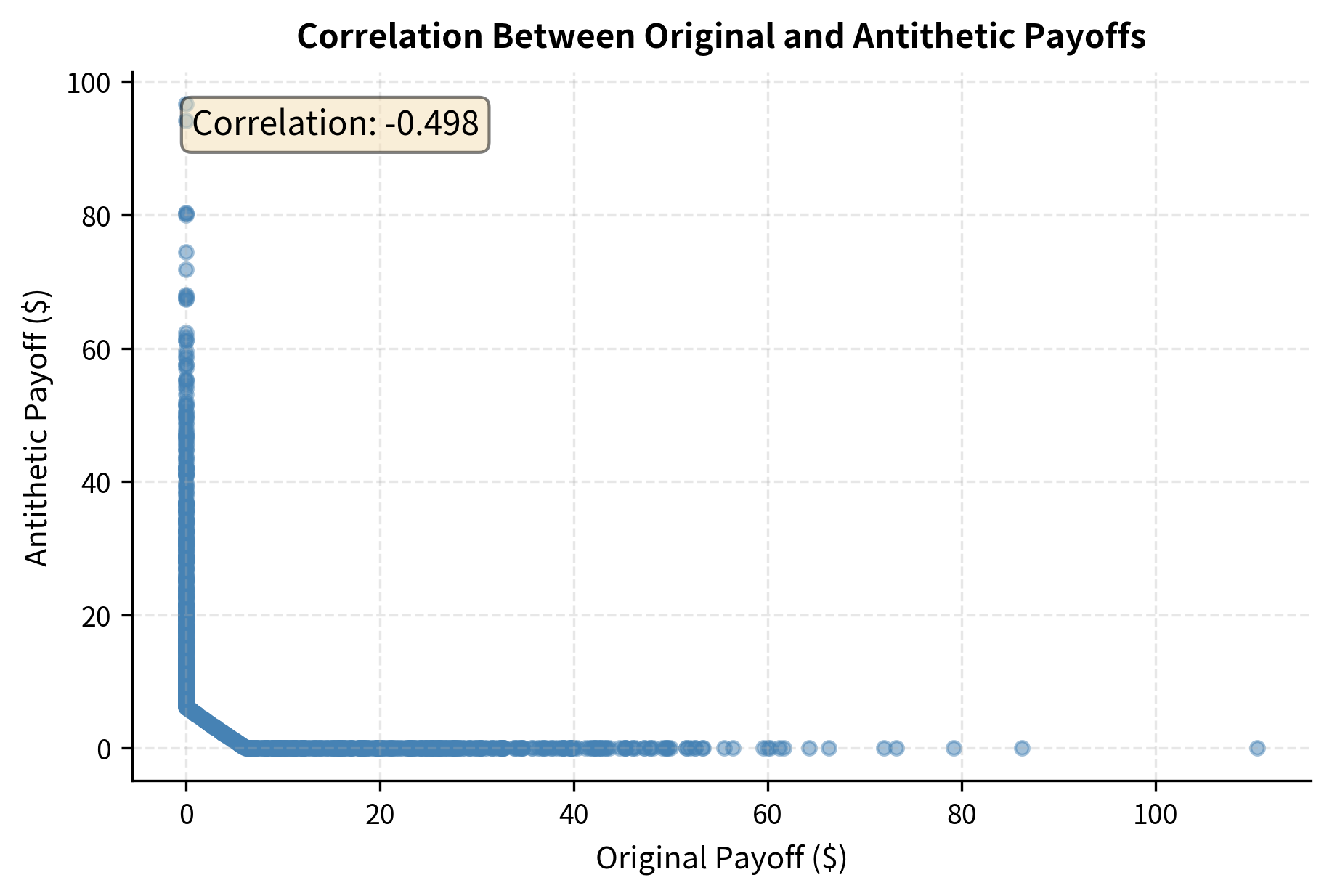
The strong negative correlation visible in the scatter plot is what drives the variance reduction. When the original path produces a large payoff, the antithetic path tends to produce a small payoff, and their average is closer to the true expected value than either would be alone.

Control Variates
Control variates adjust Monte Carlo estimates by exploiting information from related quantities with known expected values. This section presents the mathematical framework and demonstrates practical applications to option pricing.
The Core Intuition
Control variates use a different strategy: instead of modifying how we sample, we adjust our estimate using information from a related quantity whose expected value we know exactly. The idea is analogous to using a calibration standard in measurement. If we know exactly what a reference measurement should be, we can use any deviation to correct our target measurement.
To make this intuition concrete, consider a situation where you want to estimate the average height of students in a university. Suppose you also know the exact average age of all students from registration records. When you sample students, you measure both their height and age. If your sample happens to include more older students than average, the sample average height might be biased high if older students tend to be taller. But since you know the true average age, you can detect this bias in your age measurements and use it to correct your height estimate. This is precisely what control variates do.
Suppose we want to estimate but don't know its exact value. However, we have access to another random variable that is correlated with and whose expected value we do know. During each simulation, we observe both and . If happens to be above its known expected value, and and are positively correlated, then is probably also above its expected value. We can use this information to adjust our estimate of downward.
The beauty of this approach is that it exploits known information without changing the simulation procedure. We still generate the same random samples, but we extract more information from each sample by using the relationship between the target quantity and the control variable.
Mathematical Foundation
The mathematical framework for control variates formalizes the intuition of using known information to correct our estimates. The control variate estimator for is:
where:
- : control variate estimator
- : sample mean of the target variable
- : sample mean of the control variable
- : known expected value of the control variable
- : adjustment coefficient
This formula has an elegant interpretation. The term measures how much our sample of deviates from its known expectation. This deviation serves as a diagnostic: it tells us whether our particular sample is biased high or low relative to the true population. The coefficient determines how strongly we use this diagnostic information to correct our estimate of . We use this deviation to correct our estimate of .
The expected value of this estimator is:
where:
- : control variate estimator
- : sample means of target and control
- : adjustment coefficient
- : expected value of control variable
- : expected value of target variable
The estimator is unbiased for any choice of since . This is a crucial property that gives us freedom in choosing . No matter what coefficient we select, the expected value of our estimator equals the true quantity we seek. This means we can choose to minimize variance without worrying about introducing bias.
Now we analyze the variance of the control variate estimator to understand how to choose the optimal coefficient. The variance of the control variate estimator is:
where:
- : variance of the control variate estimator
- : variance of
- : variance of
- : covariance between and
- : adjustment coefficient
- : number of simulations
This expression reveals the trade-off in choosing . The first term is the variance of standard Monte Carlo. The second term adds variance proportional to how aggressively we use the control. The third term subtracts variance when and the covariance have the same sign. The optimal choice of balances the benefit of using the control against the cost of adding its variability.
To minimize variance, we take the derivative with respect to and set it to zero:
where:
- : control variate coefficient
- : number of simulations
- : variance of the control variable
- : covariance between target and control
Solving for :
where:
- : optimal control variate coefficient
- : covariance between and
- : variance of
This optimal coefficient is precisely the slope from regressing on . This connection to regression provides both intuition and practical implementation. The regression slope measures how much changes per unit change in , which is exactly what we need to know to correct for deviations in from its mean. In practice, we can estimate by running an ordinary least squares regression of on using our simulation data.
Variance Reduction with Optimal Coefficient
Having derived the optimal coefficient, we can now determine exactly how much variance reduction the control variate method achieves. Substituting back into the variance formula:
where:
- : variance of the optimized control variate estimator
- : variance of the standard Monte Carlo estimator
- : correlation between target and control
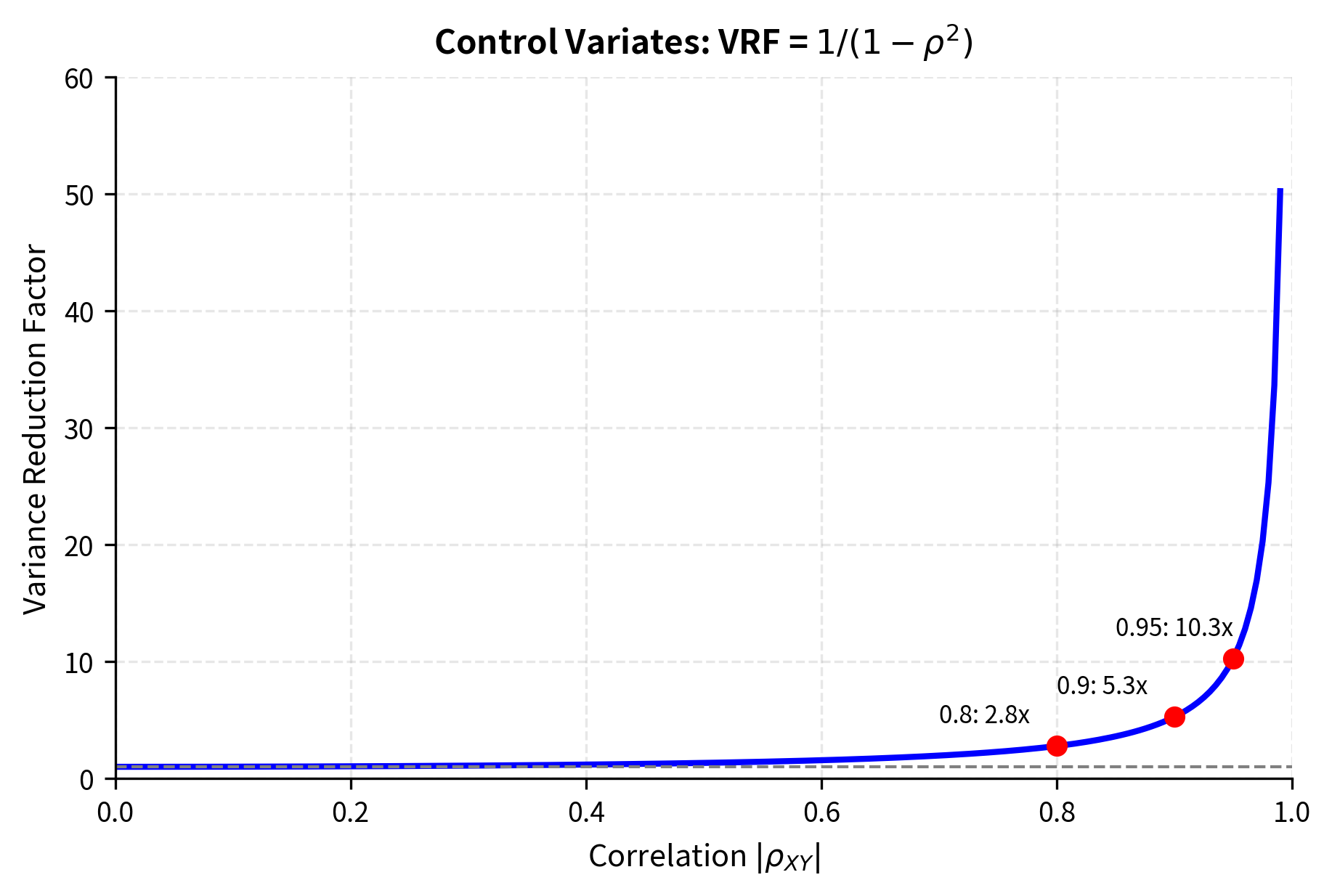
This elegant result shows that the variance is reduced by a factor of compared to standard Monte Carlo. The variance reduction factor is:
where:
- : Variance Reduction Factor
- : correlation between target and control
This formula reveals that variance reduction depends entirely on the squared correlation between and . A control variate with correlation yields a variance reduction factor of . With , the factor jumps to approximately 50. The squared correlation appearing in this formula explains why finding highly correlated controls is so valuable: the benefit grows rapidly as correlation approaches 1.
Notice that the sign of the correlation does not matter because we square it. Whether the control is positively or negatively correlated with the target, the optimal coefficient will have the appropriate sign to correct for deviations. What matters is the strength of the relationship, not its direction.
::: {.callout-note title="Optimal Control Variate Coefficient" The optimal coefficient for control variates equals the regression slope of on . In practice, we estimate this coefficient from our simulation data using ordinary least squares, which introduces a small bias but typically provides near-optimal variance reduction. :::
Choosing Control Variates for Option Pricing
The most natural control variate for option pricing is the underlying asset itself. For a call option, define:
- = discounted call option payoff =
- = discounted terminal asset price =
Under risk-neutral pricing, we know that (the current stock price). This provides a perfect control variate since:
- We observe in every simulation (we need it to compute the payoff anyway)
- The expected value is known exactly
- is highly correlated with the call payoff
The first point is particularly important from a computational perspective. Using the terminal stock price as a control adds zero additional simulation cost because we already compute to evaluate the option payoff. The information is free; we just need to use it intelligently. The second point provides the anchor that makes control variates work: the martingale property of discounted prices under the risk-neutral measure gives us exact knowledge of . The third point ensures substantial variance reduction because the call payoff is a monotonically increasing function of the terminal stock price.
Implementation for European Options
The control variate method achieves impressive variance reduction because the terminal stock price is highly correlated with the call option payoff.
![Scatter plot showing the relationship between discounted option payoffs $X$ and discounted terminal stock prices $Y$ (the control variate). Each point represents one simulated path. The red regression line indicates the optimal adjustment relationship with slope $c^* \approx 0.019$, which can be estimated from the data using ordinary least squares regression. The vertical green line marks the known expected value $\mathbb{E}[Y] = S_0 = 100$. Payoffs to the right of this line (where $Y > S_0$) are adjusted downward by the control variate correction, while payoffs to the left are adjusted upward, using the deviation of $Y$ from its known mean to improve the estimate.](https://cnassets.uk/notebooks/11_variance_reduction_files/control-variate-regression.png)
Delta-Based Control Variates
For more sophisticated control variates, we rely on the martingale property of the discounted asset price. Since is a martingale under the risk-neutral measure, the stochastic integral of the delta-hedging strategy with respect to the discounted price process has zero expectation:
where:
- : time to expiration
- : option delta at time
- : asset price at time
- : risk-free interest rate
- : change in the discounted asset price
This formula represents the expected profit from a continuously rebalanced delta hedge. The delta is the sensitivity of the option price to the underlying asset price at each instant. A perfect delta hedge should have zero expected gain because it perfectly offsets the option's risk. This theoretical result from continuous-time finance provides an ideal control variate.
Discretizing this integral gives us a control variate based on the option's delta. The intuition is that a delta-hedged option position should have zero expected gain, providing a strong control. In practice, we simulate the hedging strategy by computing the delta at each time step using the Black-Scholes formula, then accumulating the gains and losses from the hedge as the stock price evolves along the simulated path. The discrepancy between the hedge outcome and zero can be used to correct our option price estimate.
The delta-based control variate provides dramatic variance reduction because it exploits the martingale structure of the risk-neutral pricing framework.
Stratified Sampling
Stratified sampling improves Monte Carlo estimates by ensuring systematic coverage of the random input space. This section explains the approach and demonstrates its application to option pricing.
The Core Intuition
Standard Monte Carlo generates random samples that may cluster in some regions while leaving other regions undersampled. Stratified sampling forces the samples to cover the input space more evenly by dividing it into strata and sampling from each stratum. This ensures that extreme outcomes in both tails are represented, reducing variance caused by sampling fluctuations.
Consider throwing darts randomly at a target. Some areas will have many darts while others have few, purely by chance. If instead you divide the target into regions and ensure exactly one dart lands in each region, the coverage is more uniform and your estimate of "average distance from center" would be more precise. The random clustering that occurs with purely random sampling adds variance to our estimates; stratified sampling eliminates this source of variance.
To understand why clustering causes problems, imagine estimating the expected payoff of a call option using only 100 random samples. By chance, these 100 standard normal random numbers might all fall between -2 and +2, leaving the tails underrepresented. But the tails matter for option pricing because extreme moves determine whether deep out-of-the-money options finish in the money. Stratified sampling ensures that we sample from the entire distribution, including the tails, in a controlled and representative manner.
Mathematical Foundation
The mathematical analysis of stratified sampling reveals precisely why forcing uniform coverage reduces variance. Divide the sample space into non-overlapping strata with probabilities where . The stratified estimator allocates samples to stratum and computes:
where:
- : stratified estimator
- : probability of stratum
- : sample mean within stratum
- : total number of strata
This formula is a weighted average of the sample means within each stratum, with weights equal to the stratum probabilities. The stratified estimator reconstructs the overall expectation by combining the conditional expectations within each region of the sample space.
The variance of the stratified estimator (with proportional allocation ) is:
where:
- : variance of the stratified estimator
- : total number of samples
- : total number of strata
- : probability of stratum
- : variance of within stratum
This variance expression contains only the within-stratum variances. To understand the improvement, we must compare this to the variance of standard Monte Carlo. The standard Monte Carlo variance can be decomposed as:
where:
- : total variance of a single sample
- : total number of strata
- : probability of stratum
- : variance of within stratum
- : expected value within stratum
- : overall expected value
This decomposition, known as the law of total variance separates the total variance into two components. The first term is the within-stratum variance (what stratified sampling has). The second term is the between-stratum variance (what stratified sampling eliminates). Thus, stratified sampling always reduces variance, with the reduction equal to the between-stratum variance.
The between-stratum variance measures how much the stratum means differ from each other. When the function we're estimating varies significantly across the sample space, meaning different regions have very different expected values, the between-stratum variance is large. Stratified sampling eliminates this variation by guaranteeing representation from each region, removing the variance that would otherwise arise from random fluctuations in how many samples fall in each region.
Implementation for Option Pricing
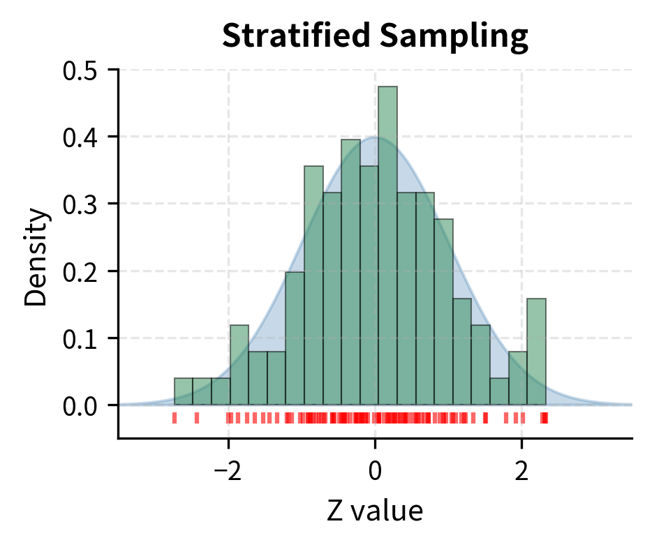
For option pricing, we stratify the uniform random variable that generates our normal random variables via the inverse CDF transform. By ensuring values are spread evenly across , we ensure the corresponding normal random variables cover the distribution evenly. This approach is particularly elegant because it works with the standard machinery of random number generation while adding the stratification benefit.
The implementation divides the unit interval into equal strata, each with probability . Within each stratum, we generate uniform random numbers that fall only within that stratum's portion of the interval. When we apply the inverse normal CDF transformation to these stratified uniform values, the resulting normal values are guaranteed to cover the entire normal distribution evenly.
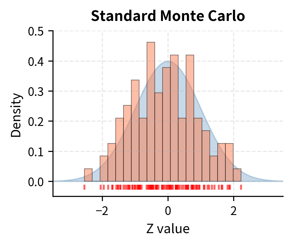
Let's compare stratified sampling to standard Monte Carlo.
Latin Hypercube Sampling
Latin Hypercube Sampling (LHS) extends stratified sampling to multiple dimensions. In standard stratified sampling for multiple variables, the number of strata grows exponentially with dimension (the curse of dimensionality LHS avoids this by ensuring each variable is stratified marginally while allowing joint flexibility.
The challenge with multi-dimensional stratification becomes apparent when we consider path-dependent options. An option that depends on 50 time steps has 50 random inputs. Full stratification would require dividing each dimension into strata, and with even 10 strata per dimension, we would need cells to cover the space, an impossibly large number. LHS provides a practical alternative that maintains the benefits of stratification without this exponential explosion.
LHS divides each input dimension into equally probable intervals and ensures exactly one sample falls in each interval for each dimension. This guarantees good marginal coverage without the exponential growth in strata that full stratification would require.
The name "Latin Hypercube" comes from the connection to Latin squares in combinatorics. A Latin square is an arrangement where each row and column contains each symbol exactly once. LHS generalizes this to higher dimensions, ensuring that when we project the samples onto any single dimension, they cover that dimension evenly with exactly one sample in each stratum.
Visualizing Sampling Coverage
The following visualization compares how different sampling methods cover the random input space.
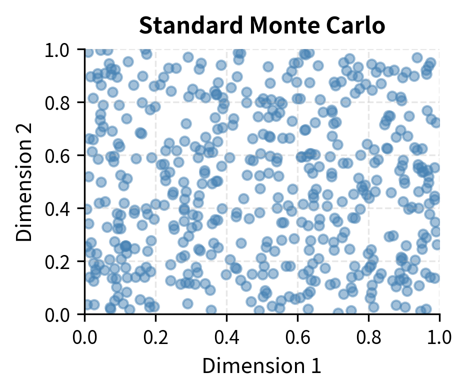
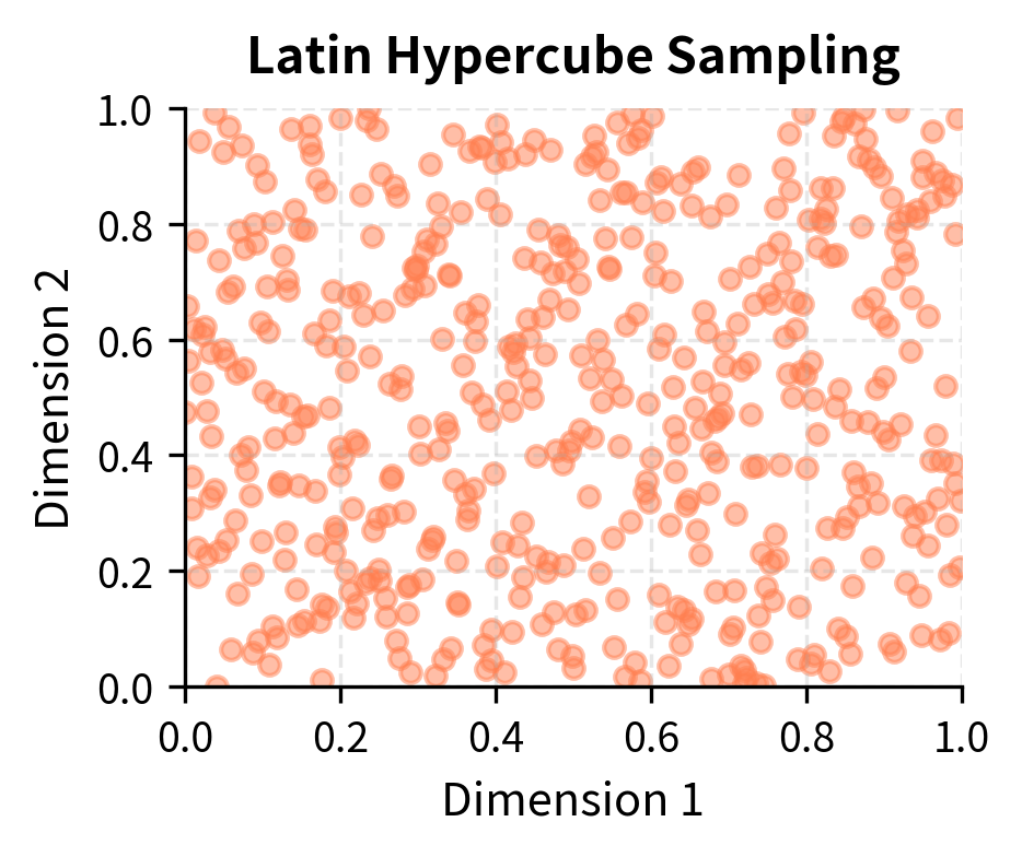
Notice how LHS provides much more uniform coverage of the unit square. This uniformity translates directly into reduced variance for estimating integrals over this space.
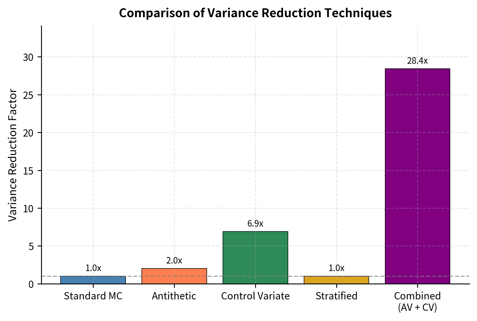
Combining Variance Reduction Techniques
The techniques we've covered are not mutually exclusive. In practice, combining multiple methods can yield variance reduction factors far exceeding what any single technique achieves alone.
Antithetic Variates + Control Variates
The combined method achieves variance reduction factors that exceed the sum of individual improvements, demonstrating how these techniques complement each other.
Convergence Analysis
Understanding how variance reduction affects convergence helps in practical deployment. Let's visualize the convergence of different methods.
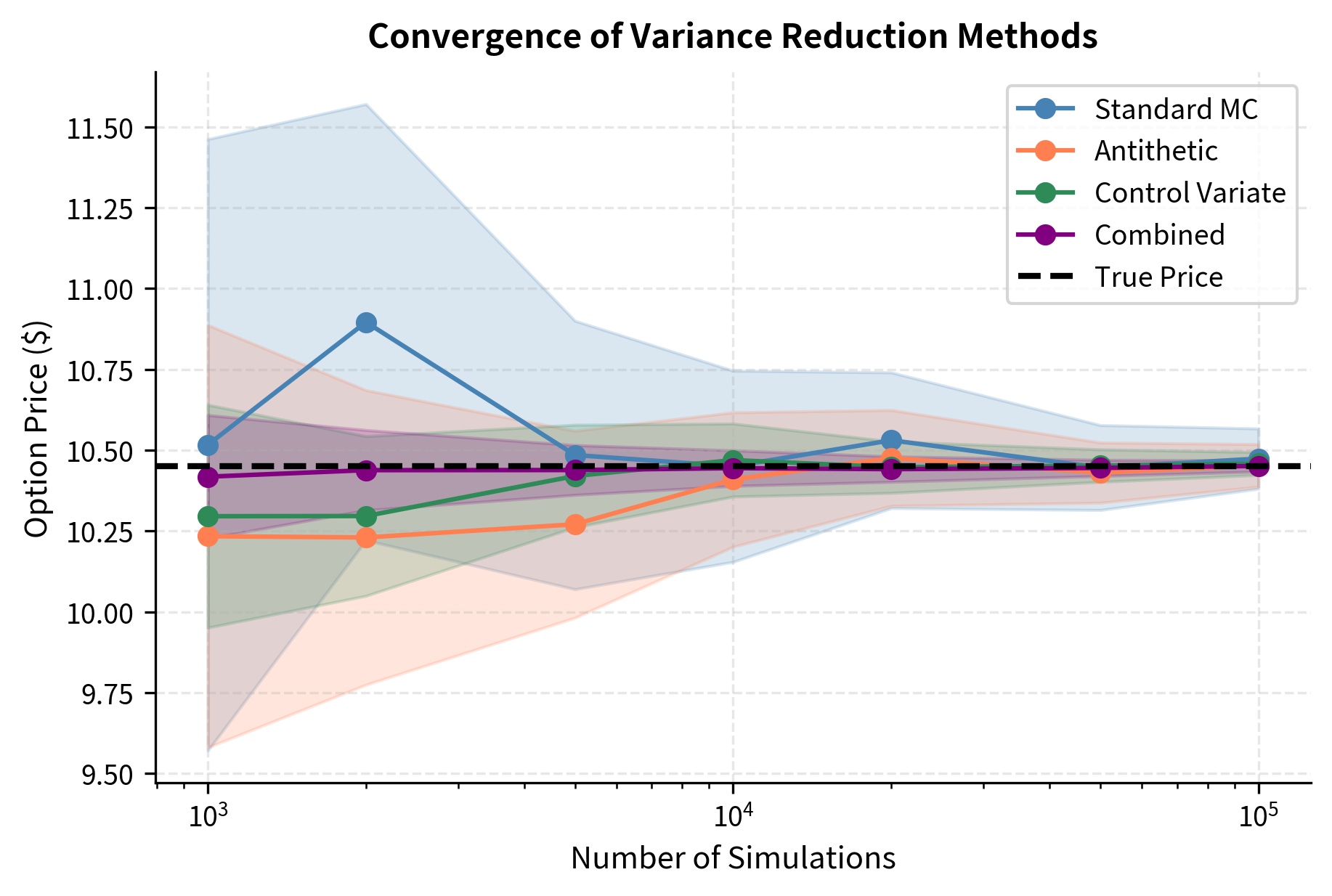
The shaded regions show 95% confidence intervals (two standard errors). Methods with stronger variance reduction have tighter confidence intervals, reaching the same precision with fewer simulations.

Computational Efficiency Comparison
When choosing a variance reduction technique, we must consider not just variance reduction but also computational overhead. Some methods (like delta-based control variates) require additional calculations that increase the cost per simulation.
The efficiency metric accounts for both variance reduction and computational cost. A method with high VRF but also high computational overhead may not be the most efficient choice.
Practical Considerations and Guidelines
Selecting and implementing variance reduction techniques requires balancing theoretical benefits against practical constraints. This section provides guidance for you.
Choosing the Right Technique
The best variance reduction technique depends on the problem structure:
-
Antithetic variates work best for monotonic payoff functions. They are simple to implement and add minimal computational overhead. Use them as a default first step.
-
Control variates excel when you have access to related quantities with known expectations. The underlying asset price is a natural control for many options. More sophisticated controls (delta-based, basket components) provide larger reductions but require more computation.
-
Stratified sampling is most effective for low-dimensional problems where the payoff varies significantly across the input space. LHS extends this to moderate dimensions.
Combining Techniques
A practical approach is to layer techniques:
- Start with antithetic variates (easy, low overhead)
- Add a simple control variate (underlying asset price)
- Consider stratified sampling for path-independent options
- For exotic options, explore delta-based or more sophisticated controls
Estimating Variance Reduction
Always estimate your variance reduction factor empirically. The theoretical formulas depend on correlations that may differ from expectations. Run a pilot study with a subset of simulations to estimate the improvement before committing to a full production run.
::: {.callout-warning title="Practical Caution" Variance reduction factors estimated from finite samples have uncertainty. A method that appears to reduce variance by 10x on a pilot study of 10,000 simulations might only achieve 7x reduction on the full run. Budget conservatively. :::
Limitations and Impact
Variance reduction techniques have transformed Monte Carlo simulation from a computationally expensive necessity into a practical tool for real-time pricing and risk management. However, these methods come with important limitations that you must understand.
The effectiveness of variance reduction varies dramatically with the problem structure. Antithetic variates provide consistent but moderate improvement for most options, but their benefit disappears for symmetric payoffs like straddles. Control variates can achieve spectacular variance reduction when strong controls exist, but finding good controls for exotic path-dependent derivatives requires insight into the problem structure; there is no automatic procedure that works universally. The delta-based control we implemented requires computing option deltas at each time step, which adds substantial computational cost and may not be worthwhile for simple European options where other methods suffice.
Stratified sampling faces the curse of dimensionality. For a single-asset European option, stratifying the terminal random variable works beautifully. But for a path-dependent option with 252 daily time steps, the effective dimension is far higher, and naive stratification becomes impractical. title="Latin Hypercube Sampling" helps but provides diminishing returns as dimension increases. For very high-dimensional problems, quasi-random sequences (which we'll explore in later chapters) may be more effective.
Another limitation is that combining techniques doesn't always multiply their benefits. The correlation structure that makes antithetic variates effective may already capture some of the information that a control variate would use, leading to overlap in variance reduction. The combined method is almost always better than either alone, but rarely twice as good.
Despite these limitations, variance reduction has had profound practical impact. Real-time risk calculations that would be impossible with standard Monte Carlo become feasible when variance reduction cuts required simulations by a factor of 100. Model calibration, which requires many option evaluations, becomes tractable. The techniques have enabled the pricing and risk management of exotic derivatives that would otherwise be computationally intractable.
Looking ahead, the finite difference methods covered in the next chapter provide an alternative approach for lower-dimensional problems, while exotic option pricing will require careful selection of variance reduction strategies tailored to specific payoff structures.
Summary
This chapter introduced three fundamental variance reduction techniques that dramatically improve Monte Carlo simulation efficiency:
Antithetic variates exploit the symmetry of the normal distribution by pairing simulations using and . The negative correlation between pairs reduces variance for monotonic payoffs. Implementation is straightforward: generate half as many random numbers and use each twice with opposite signs.
Control variates adjust Monte Carlo estimates using related quantities with known expectations. The optimal adjustment coefficient equals the regression slope of the target variable on the control. The discounted terminal stock price provides a natural control for option pricing, with delta-based controls offering even larger improvements at greater computational cost.
Stratified sampling ensures uniform coverage of the random input space by dividing it into strata and sampling from each. Latin Hypercube Sampling extends this to multiple dimensions without exponential growth in strata.
Key takeaways for practice:
- Start simple. Implement antithetic variates first since they add minimal overhead and work for most options.
- Exploit known expectations. Look for control variates with high correlation to your target.
- Combine techniques. Layer multiple methods for multiplicative benefits.
- Benchmark empirically. Theoretical variance reduction may not match reality.
- Consider computational cost. The best method balances variance reduction against time per simulation.
The variance reduction factor tells you how many times fewer simulations you need. A VRF of 10 means the same accuracy in one-tenth the time, a transformation that makes real-time derivatives pricing possible.
Quiz
Ready to test your understanding? Take this quick quiz to reinforce what you've learned about variance reduction techniques in Monte Carlo simulation.

Comments