

Master exotic options pricing including Asian, barrier, lookback, and digital options. Learn closed-form solutions and Monte Carlo simulation methods.
Choose your expertise level to adjust how many terms are explained. Beginners see more tooltips, experts see fewer to maintain reading flow. Hover over underlined terms for instant definitions.
Exotic Options and Complex Derivatives
The vanilla European and American options we explored in earlier chapters form the foundation of derivatives markets, but they represent only a fraction of the contracts traded in practice. Financial engineers have developed a rich ecosystem of exotic options with customized payoff structures designed to meet specific hedging needs, express precise market views, or reduce premium costs compared to vanilla alternatives.
Exotic options differ from their vanilla counterparts by incorporating additional features. Path dependence means the payoff depends on the entire price history, not just the terminal value. Other features include multiple exercise opportunities, barrier conditions that activate or deactivate the option, and payoffs linked to averages, extrema, or other statistics of the underlying price path. These features create hedging tools that more precisely match corporate exposures, offer attractive yield profiles in structured products, and help traders capture nuanced market views.
The pricing of exotics draws heavily on the techniques you have already mastered. The risk-neutral valuation framework from Chapter 4 of this part applies directly: the fair price is the discounted expected payoff under the risk-neutral measure. For some exotics, this expectation admits closed-form solutions. For many others, we must rely on the Monte Carlo methods from Chapter 10 or the finite difference techniques from Chapter 12. Understanding when each approach applies, and why, is central to working with exotic derivatives.
Path-Dependent Options
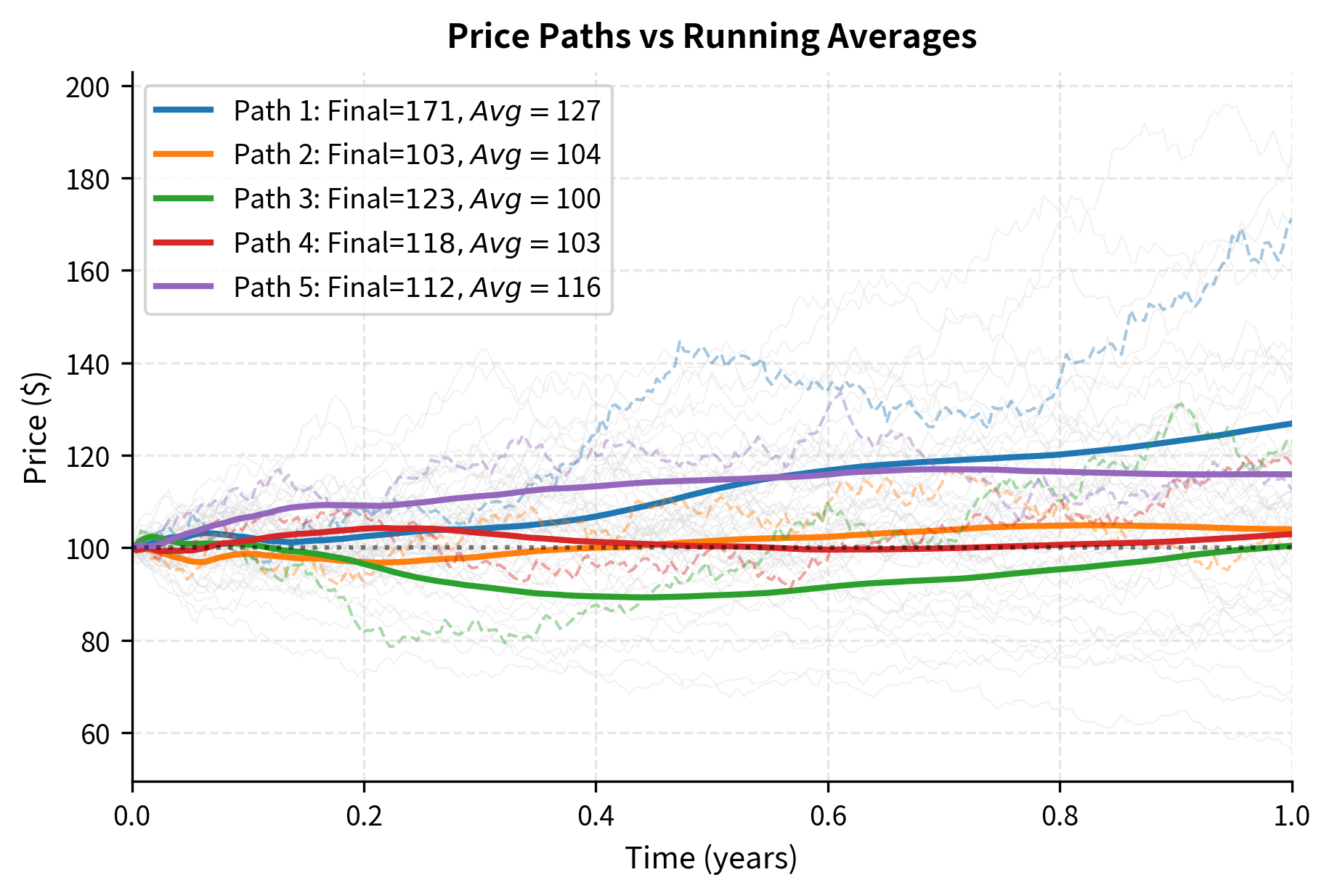
Path-dependent options have payoffs determined by the entire trajectory of prices over the option's life, not just the final price. This path dependence arises from payoffs tied to averages, maximum or minimum values, or the crossing of specific price levels during the option's life.
To understand why path dependence matters, consider a simple thought experiment. Imagine two stocks that both start at $100 and end at $110. For a vanilla European call with strike $100, both stocks produce the same $10 payoff. But suppose the first stock rose steadily from 110, while the second spiked to 110. A lookback option holder caring about the maximum price would receive very different payoffs from these two paths. The terminal prices are identical, yet the payoffs differ substantially. This sensitivity to the journey, not just the destination, defines path-dependent options and creates both their value and their pricing complexity.
Asian Options
Asian options (also called average options) have payoffs based on the average price of the underlying asset over some period, rather than the spot price at expiration. This averaging feature reduces volatility in the payoff and makes the option less susceptible to manipulation or extreme price movements near expiration.
The intuition behind Asian options becomes clear when you consider what averaging actually does mathematically. By taking the mean of many price observations, you create a random variable with lower variance than any single observation. The central limit theorem tells us that averages of independent draws converge to a normal distribution. While stock prices are not independent across time, the averaging still substantially dampens extreme outcomes. A single day's price spike has limited impact when averaged with 251 other daily observations.
Variants:
- Average price options: The average replaces the spot price in the payoff formula. A call pays where is the average price.
- Average strike options: The average replaces the strike price. A call pays .
The averaging can be computed as either an arithmetic mean or a geometric mean of sampled prices:
where:
- : asset price at monitoring time
- : number of monitoring points
- : arithmetic mean of prices
- : geometric mean of prices
The distinction between arithmetic and geometric averages has profound implications for pricing. The arithmetic average, which simply sums the prices and divides by the count, represents what most people intuitively think of as an average. It matches how businesses actually compute their average costs or revenues over time. The geometric average, computed by multiplying all prices together and taking the nth root, is always less than or equal to the arithmetic average (a fact known as the AM-GM inequality), with equality only when all prices are identical. While the geometric average may seem less natural, it has a remarkable mathematical property that makes it analytically tractable. The geometric mean of lognormally distributed random variables is itself lognormally distributed, preserving the distributional assumptions that underpin the Black-Scholes framework.
Asian options are heavily used in commodity markets where corporations need to hedge their average cost of inputs over a month or quarter. An airline hedging jet fuel costs cares about the average price paid over the year, not the spot price on December 31st. Similarly, they appear in currency markets for hedging translation exposure on revenues received throughout a period.
Pricing Asian Options
The geometric average of lognormal prices is itself lognormal, which allows a closed-form solution for geometric Asian options. This mathematical convenience arises from a fundamental property of logarithms: the logarithm of a product equals the sum of logarithms. Since the logarithm of each price in our geometric Brownian motion model is normally distributed, and the geometric average involves taking the nth root of a product (equivalently, averaging the logarithms), the result remains in the lognormal family.
If the underlying follows geometric Brownian motion, the geometric average has the distribution:
where:
- : geometric mean of prices
- : adjusted mean of the logarithmic distribution
- : adjusted variance of the logarithmic distribution
The adjusted mean and variance account for the averaging. The closed-form price uses the Black-Scholes formula with modified parameters.
For geometric Asian call options with continuous averaging:
where:
- : current stock price
- : strike price
- : risk-free rate
- : time to maturity
- : volatility
- : dividend yield
- : adjusted mean for the average
- : adjusted variance for the average
- : standardized distance measure
- : risk-adjusted distance measure
- : cumulative standard normal distribution
This formula mirrors the Black-Scholes structure, where represents the expected value of the geometric average price.
Examine the key adjustments in this formula more carefully. The adjusted mean contains the factor rather than because averaging over the entire period effectively halves the exposure to drift. Think of it this way. Prices at the beginning of the averaging window have the full time period to drift, while prices at the end have almost no time to drift. On average, each price observation experiences drift for half the total time. The adjusted variance reflects a similar but more subtle effect. The factor of arises from integrating the variance contribution across the averaging period, and it captures how averaging reduces volatility exposure. Each price observation contributes to the variance, but since the observations are correlated (they all stem from the same underlying price path), the variance reduction is not as dramatic as it would be for independent observations.
Arithmetic Asian options have no closed-form solution because the sum of lognormal random variables is not lognormal. In practice, they are priced using Monte Carlo simulation or by using the geometric price as a control variate, as we discussed in Chapter 11.
The geometric Asian call price of $3.52 is lower than a comparable vanilla European call would be because the averaging reduces the option's exposure to extreme price movements. This reduction in volatility exposure makes Asian options particularly attractive when hedging average exposures over time.
Let's compare this to pricing via Monte Carlo simulation, which also handles the arithmetic case:
The Monte Carlo price for the geometric Asian of 3.85, approximately 9% more expensive than the geometric Asian. This difference arises because the arithmetic average is always greater than or equal to the geometric average by the AM-GM inequality. Both Asian options are cheaper than a corresponding vanilla European call, which for these parameters would be priced around $10.45. The substantial discount reflects how averaging reduces exposure to extreme price movements and therefore lowers option value.
Barrier Options
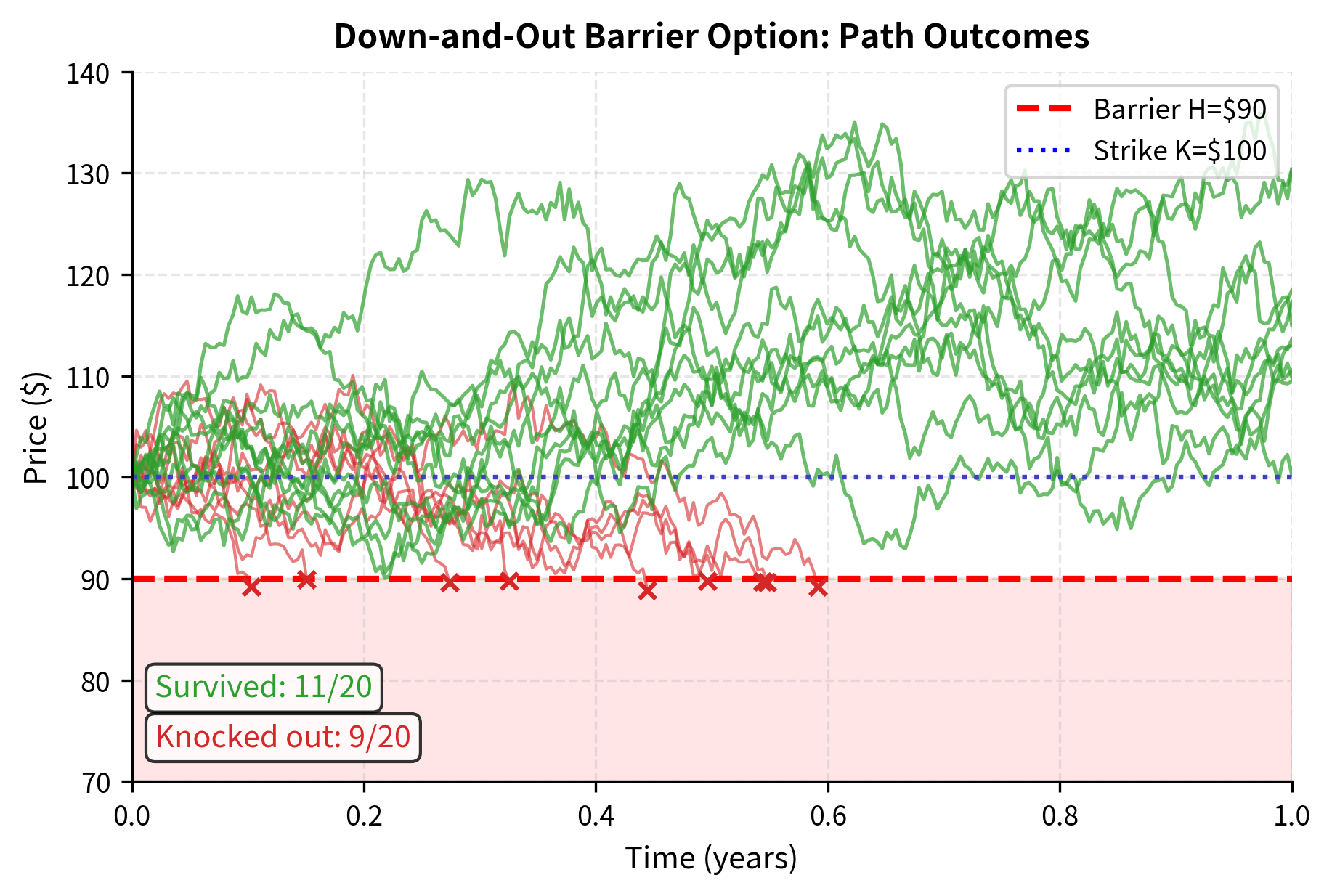
Barrier options are activated (knocked in) or extinguished (knocked out) when the underlying price crosses a specified barrier level during the option's life. They offer the same terminal payoff as vanilla options but at a lower premium because the payoff is contingent on the path avoiding (or reaching) the barrier.
The fundamental insight behind barrier options is that they partition the universe of possible price paths into two sets: those that cross the barrier at some point, and those that do not. By making the option payoff contingent on which set the realized path belongs to, we create an instrument whose value depends not just on where the price ends up, but on where it traveled along the way. This path dependence allows buyers to pay only for the scenarios they care about, reducing premium costs when they're willing to accept the knockout risk.
The four basic types are:
- Down-and-out: Option expires worthless if price falls below barrier H < S₀
- Down-and-in: Option activates only if price falls below barrier H < S₀
- Up-and-out: Option expires worthless if price rises above barrier H > S₀
- Up-and-in: Option activates only if price rises above barrier H > S₀
Each can be applied to calls or puts, creating eight fundamental barrier option types.
A key relationship links knock-in and knock-out options to vanilla options:
where:
- : value of the barrier option that activates if the barrier is crossed
- : value of the barrier option that extinguishes if the barrier is crossed
- : value of the corresponding standard option without barrier features
This in-out parity holds because the underlying price either crosses the barrier during the option's life or does not. If it crosses, the knock-in activates and the knock-out extinguishes. If it does not cross, the knock-out survives and the knock-in never activates. Either way, exactly one of the barrier options pays off identically to the vanilla option.
This relationship is model-independent. Regardless of how we model the underlying price dynamics, the dichotomy between paths that hit the barrier and paths that do not exhausts all possibilities. This means we can always price one type of barrier option if we know the vanilla price and the price of its complementary barrier type. In practice, this relationship serves as both a pricing tool and a consistency check for models.
Closed-Form Barrier Option Pricing
Under the Black-Scholes assumptions, closed-form solutions exist for European barrier options. The formulas are algebraically involved but follow from applying the reflection principle and the risk-neutral pricing framework.
The reflection principle is a powerful technique from the theory of Brownian motion that allows us to count paths hitting a barrier. The key insight is the following. For every path that starts at , hits the barrier at some time, and ends at , there exists a corresponding "reflected" path that starts at , hits the barrier, and ends at (the reflection of about the barrier level, when working in log-space). This bijection between paths allows us to express the probability of hitting the barrier in terms of terminal distributions. We can compute these probabilities using our lognormal price assumptions.
For a down-and-out call with barrier and :
where:
- : standard Black-Scholes call price
- : current stock price
- : strike price
- : barrier level ()
- : risk-free rate
- : time to expiration
- : volatility
- : shape parameter related to drift and volatility
- : standardized barrier distance parameter
- : cumulative standard normal distribution
The formula decomposes into the vanilla price minus a barrier adjustment:
- is the price of an otherwise identical vanilla call option.
- The barrier adjustment consists of the remaining terms, which quantify the value of paths that hit the barrier . The factor arises from the reflection principle, adjusting the probability measure for trajectories that touch the barrier.
The parameter captures the relationship between the drift rate (under the risk-neutral measure) and the diffusion rate of the underlying process. When is large, the drift dominates diffusion, meaning the price tends to move directionally rather than randomly. When is small, randomness dominates, and the price is more likely to wander and potentially hit barriers. The power can be interpreted as a likelihood ratio that accounts for how the drift affects the probability of reaching the barrier.
The standardized distance parameter measures how far the barrier is from the current price in a normalized sense. The term appearing in the logarithm relates to the reflection principle: it represents where a path reflected about the barrier would need to end up to produce a positive payoff. The adjustment shifts this measure to account for the drift over the option's lifetime.
The down-and-out call costs $6.23 compared to $10.45 for the vanilla call, a discount of approximately 40%. This substantial reduction reflects the risk-neutral probability of the stock price touching the $90 barrier (10% below current spot) during the one-year life of the option. If the barrier is hit at any point, the option is extinguished and becomes worthless regardless of where the stock price is at expiration. The down-and-in call, priced at $4.22, represents the complementary value and together with the down-and-out call sums to the vanilla call price, demonstrating the in-out parity relationship.
Let's visualize how barrier option prices depend on the barrier level:
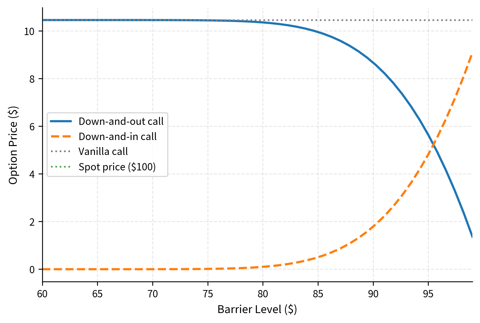
As the barrier approaches the current spot price, the down-and-out option becomes nearly worthless because it is almost certain to knock out. Meanwhile, the down-and-in option converges to the vanilla price because it is almost certain to knock in.
Lookback Options
Lookback options have payoffs based on the maximum or minimum price achieved by the underlying asset during the option's life. They eliminate the regret of missing the optimal exercise moment.
Lookback options address the challenge of optimal timing: when should you capitalize on favorable price movements? With a vanilla call, you receive the terminal price minus the strike. For example, if the stock reached 110 at expiration, you captured some gain, but not the maximum possible. Lookback options solve this problem by automatically locking in the best price achieved, removing the need for perfect market timing.
The two main variants are:
- Floating strike lookback call: Pays , where is the minimum price during the option's life. The holder effectively buys at the lowest price.
- Fixed strike lookback call: Pays , where is the maximum price. The holder benefits if the asset ever exceeded the strike.
Lookback options are expensive because they capture the most favorable price realization over the entire path. The floating strike lookback call, for instance, always has positive intrinsic value at expiration (as long as there was any price variation).
For a floating strike lookback call under Black-Scholes assumptions, the closed-form price is:
where:
- : current stock price
- : minimum observed price during the option's life
- : risk-free rate
- : time to expiration
- : volatility
- : cumulative standard normal distribution
The first term, , resembles a standard call component, while the subsequent terms adjust for the floating strike mechanics, capturing the value of the "minimum price" guarantee.
This formula reveals the interplay between several value components. The term represents the expected benefit from the terminal stock price, similar to its role in the Black-Scholes formula. The second term involving captures a correction related to the running minimum's behavior under drift. This ratio of variance to twice the drift rate appears naturally when analyzing the distribution of the minimum of a drifting Brownian motion. The third term involving represents the "cost" of the minimum already observed, adjusted for the probability that the stock will establish a new minimum before expiration.
The parameter measures how far the current price is above the observed minimum in standardized units, adjusted for the expected drift. When is much larger than (meaning the stock has already risen substantially from its low), becomes large and approaches 1, indicating high probability of finishing above the current minimum. The parameter differs from in that it uses rather than in the drift adjustment, reflecting the need to consider the dynamics under the "stock measure" where the stock itself serves as numeraire.
For newly issued lookback options , which simplifies the formula.
The floating strike lookback call is priced at $21.38, while the ATM vanilla call costs $10.45, making the lookback option 2.05 times more expensive. This substantial premium of $10.93 above the vanilla call compensates for the guarantee that the holder can effectively "buy at the low": the payoff is always ST minus the minimum price observed over the entire year. Unlike the vanilla call which locks in today's price as the strike, the lookback option eliminates all timing risk by automatically adjusting the strike to the most favorable level observed. This makes the lookback option always finish in-the-money (assuming any price variation occurs), explaining why it commands such a significant premium.
Non-Path-Dependent Exotics
Not all exotic options depend on the path of prices. Some have modified payoff structures at expiration or involve options on options.
Digital (Binary) Options
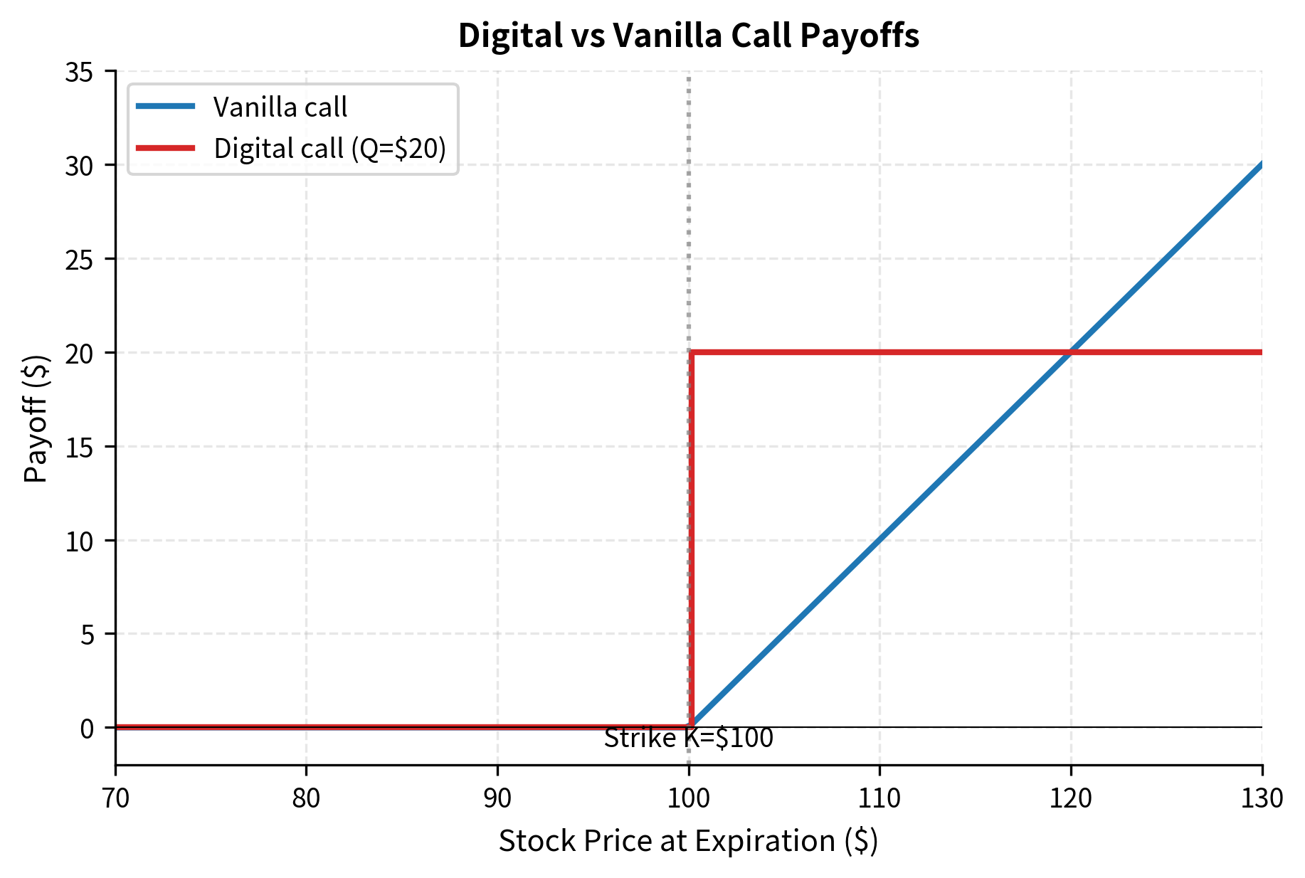
Digital options (also called binary options) have discontinuous payoffs. They pay a fixed amount if the underlying finishes above (for a call) or below (for a put) the strike price, and zero otherwise.
The defining characteristic of digital options is their all-or-nothing nature. Unlike vanilla options where the payoff scales with how far in-the-money the option finishes, digital options pay the full amount for any positive intrinsic value, no matter how small. This creates a discontinuity at the strike. One cent in-the-money, you receive the full payout. One cent out-of-the-money, you receive nothing.
For a cash-or-nothing digital call paying amount :
where is the fixed cash payout amount, is the underlying asset price at expiration, and is the strike price.
Under risk-neutral pricing, the value is:
where:
- : current stock price
- : strike price
- : cash payout amount
- : volatility
- : risk-free rate
- : time to expiration
- : distance to strike in standard deviations (risk-adjusted)
- : risk-neutral probability that the option finishes in-the-money
This is simply the present value of the cash amount times the risk-neutral probability of finishing in-the-money.
This formula has a direct probabilistic interpretation. The term represents the probability, under the risk-neutral measure, that the stock price will exceed the strike at expiration. This is the same that appears in the Black-Scholes formula, but here it stands alone rather than being multiplied by other terms. The option value is the payout amount (), discounted to present value (), times the probability of receiving it (). No other option pricing formula offers such a transparent connection between probability and price.
For an asset-or-nothing digital call that pays the asset itself if :
where:
- : current stock price
- : strike price
- : risk-free rate
- : time to expiration
- : volatility
- : standardized distance measure
- : factor adjusting for the conditional expectation of the asset price
The asset-or-nothing formula uses rather than , and this difference is mathematically significant. While gives the probability of finishing in-the-money, incorporates an additional adjustment that accounts for the correlation between the probability of exercise and the value received upon exercise. When the stock price is high (making in-the-money more likely), the asset payment is also worth more. This positive correlation means we cannot simply multiply the expected asset value by the exercise probability. Instead, represents the exercise probability under the "stock measure," which naturally accounts for this correlation.
A vanilla European call can be decomposed as long one asset-or-nothing call, short cash-or-nothing calls. This decomposition is useful for understanding how digital options contribute to vanilla option hedging.
Digital option prices decrease as the strike moves away from the current spot price. For the $95 strike (in-the-money), the cash-or-nothing call is priced at $0.53, while for the $105 strike (out-of-the-money) it drops to $0.41. These values represent the discounted risk-neutral probabilities of finishing in-the-money. The ATM strike at $100 is priced at $0.47, reflecting approximately a 50% risk-neutral probability (after time value discounting) of the stock finishing above the strike. The asset-or-nothing calls show a similar pattern: $56.59 for the $95 strike, $53.17 for ATM, and $49.88 for the $105 strike. These values incorporate both the probability of finishing in-the-money and the conditional expectation of the asset price given that outcome.
Let's verify the decomposition relationship:
The digital option decomposition exactly replicates the vanilla call price.
Hedging Challenges with Digital Options
Digital options present significant hedging challenges due to their discontinuous payoffs. As expiration approaches, the delta of a digital call near the strike becomes extremely large: a small price movement can change the payoff from zero to the full payout amount.
The mathematical reason for this hedging difficulty relates to the derivative of the cumulative normal distribution. The delta of a cash-or-nothing call is proportional to the normal density function evaluated at , divided by the time to expiration and the spot price. As expiration approaches, this division causes the delta to explode when the spot price is near the strike. In the limit, the delta becomes a Dirac delta function at the strike price, which is impossible to hedge in practice.
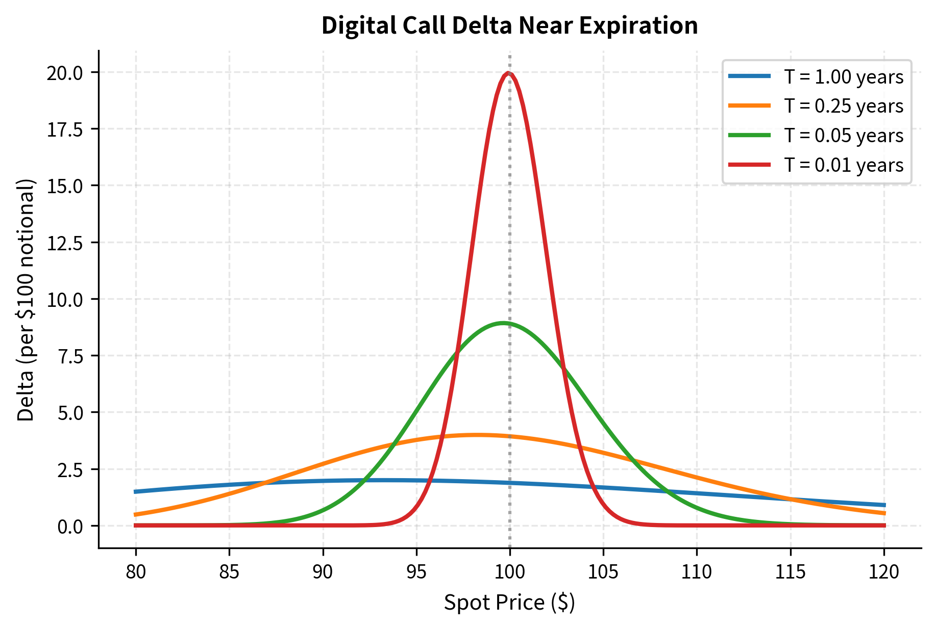
This delta explosion near expiration creates practical hedging problems. A market maker selling digital options near the strike at short maturities faces the prospect of needing to trade enormous amounts of the underlying for small price movements, incurring substantial transaction costs.
Compound Options
Compound options are options on options, where the underlying asset is itself an option. This structure creates a two-stage exercise decision.
Compound options present interesting valuation challenges. At the first expiration date, the holder decides whether to pay the compound strike to acquire the underlying option. This decision depends on the underlying option's value at that time, which depends on the stock price. However, the underlying option retains time value and depends on how the stock price will evolve until the second expiration. This creates a chain of contingent decisions that must be valued simultaneously.
The four basic types are:
- Call on call (CoC): Right to buy a call option at a specified price
- Call on put (CoP): Right to buy a put option
- Put on call (PoC): Right to sell a call option
- Put on put (PoP): Right to sell a put option
Consider a call on call with compound strike expiring at , written on an underlying call with strike expiring at , where . At , the holder of the compound option will exercise if the value of the underlying call exceeds .
where:
- : asset price at compound option expiration
- : value of the underlying European call option
- : strike price of the compound option (price to buy the underlying)
- : strike price of the underlying option
- : expiration of the compound option
- : expiration of the underlying option
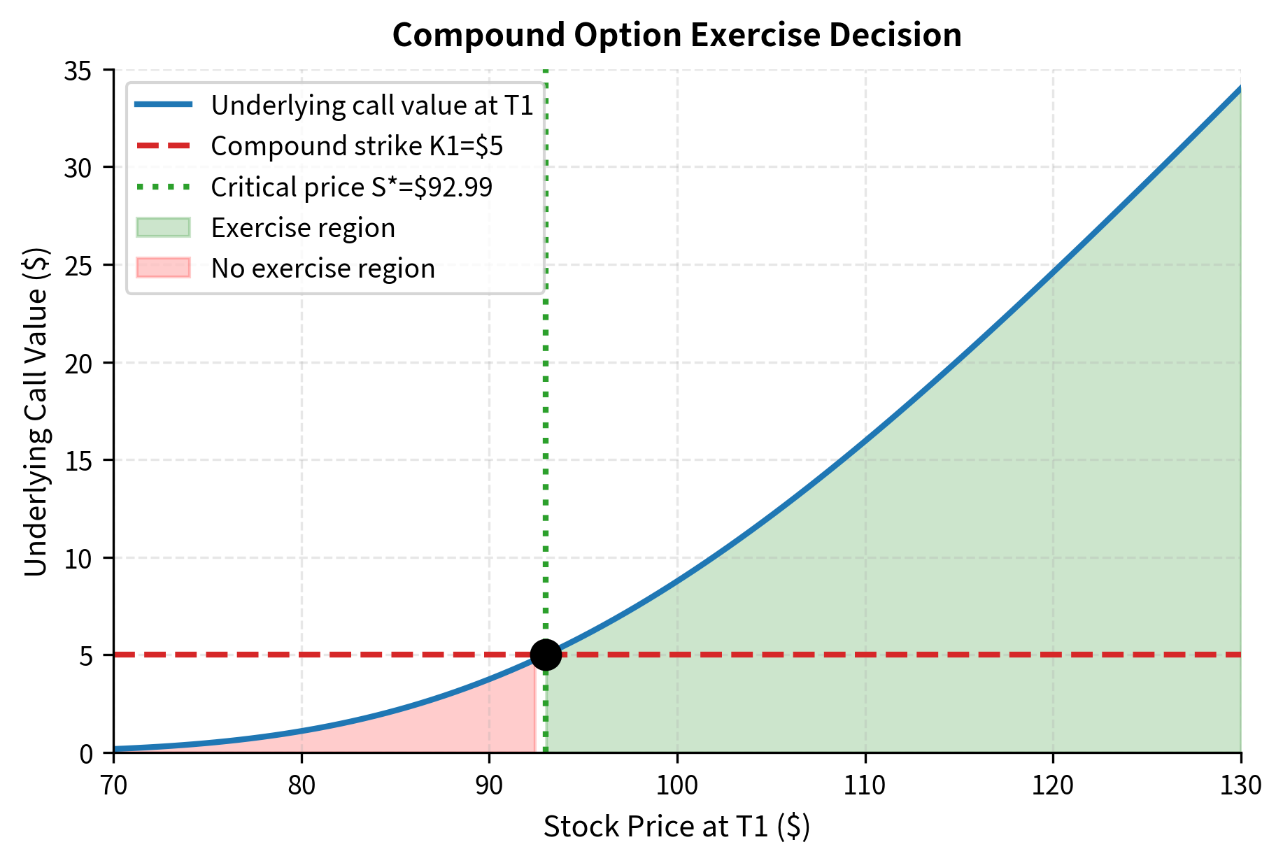
A critical stock price exists at time where the underlying option is worth exactly . For a call on call, the compound option is exercised if and only if . Finding this critical price requires solving .
The critical stock price plays a central role in compound option pricing. It divides the state space at time into two regions: when , the underlying call is worth more than and it makes sense to exercise the compound option; when , the underlying call is worth less than and the compound option expires worthless. Finding requires solving a nonlinear equation, as the Black-Scholes formula gives option value as a complex function of the stock price. Fortunately, since call prices are monotonically increasing in the stock price, a unique solution always exists and can be found efficiently using root-finding algorithms.
The closed-form pricing formula for a call on call involves the bivariate normal distribution:
where:
- : current stock price
- : strike price of the compound option
- : strike price of the underlying option
- : expiration of the compound option
- : expiration of the underlying option
- : critical stock price at where underlying option value equals
- : risk-free rate
- : volatility
- : bivariate standard normal cumulative distribution function
- : cumulative standard normal distribution
- : correlation coefficient
The formula consists of three value components.
- : The current asset price weighted by the joint probability of exercising both options (under the stock measure).
- : The present value of the underlying strike , contingent on both exercises.
- : The present value of the compound strike , contingent on exercising the compound option.
The appearance of the bivariate normal distribution reflects the joint nature of the exercise decisions. We need to compute the probability that two conditions are both satisfied: the stock price exceeds at time (triggering exercise of the compound option), and the stock price exceeds at time (making the underlying call finish in the money). These two events are correlated because they both depend on the evolution of the same underlying stock price. The correlation coefficient captures this dependence, representing how much of the total uncertainty about the terminal price at is already resolved by time .
The parameters and relate to the first exercise decision at , measuring the standardized distance from the current price to the critical price . The parameters and relate to the second exercise decision at , measuring the standardized distance from the current price to the underlying strike . The subscript 1 versions incorporate the extra drift adjustment associated with the stock measure, while the subscript 2 versions use the risk-neutral measure directly.
The call on call is priced at $7.12, while the underlying one-year call costs $10.45. At 68.1% of the underlying call value, this compound option provides a way to defer the $5 decision cost for three months. If at the three-month mark the underlying call is worth more than $5, exercising the compound option makes sense: you pay $5 to acquire a call then worth more than that amount. If the call is worth less than $5, you let the compound option expire and avoid overpaying. This structure is particularly useful when facing uncertain future hedging needs, such as in project finance where a company may need to hedge foreign exchange exposure only if a contract is awarded, or in real options applications where investment timing is flexible.
Pricing Exotic Options with Monte Carlo
When closed-form solutions aren't available, or when you want to handle complex features like multiple barriers, partial averaging windows, or general path dependencies, Monte Carlo simulation provides a flexible framework. The general approach involves:
- Simulate many paths of the underlying price under the risk-neutral measure
- Calculate the payoff for each path based on the exotic option's rules
- Discount the average payoff to obtain the price
Let's implement a comprehensive exotic option pricer using Monte Carlo:
These Monte Carlo prices confirm the patterns we observed in the closed-form solutions. The arithmetic Asian call is priced at $3.83 versus $3.52 for the geometric Asian, showing the arithmetic average premium of about 9%. The down-and-out barrier call at $6.15 reflects a 41% discount from a vanilla call due to knockout risk when the price falls below 90. The up-and-out barrier call at $8.41 shows a smaller 20% discount since the barrier at 120 is further from the current spot. The floating strike lookback at $21.35 confirms the substantial premium for path-tracking features, costing over twice the vanilla call price. The narrow confidence intervals, with standard errors around $0.01-0.03, demonstrate that 100,000 simulation paths provide good precision for these exotic option prices.
Let's visualize the payoff distributions for different exotic option types:
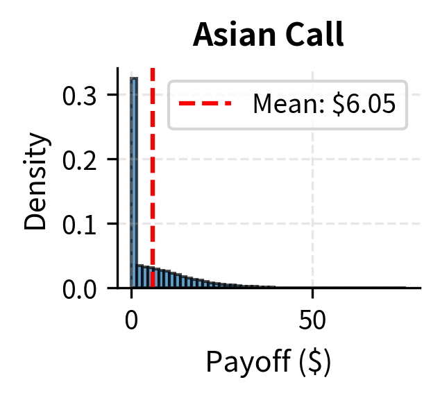
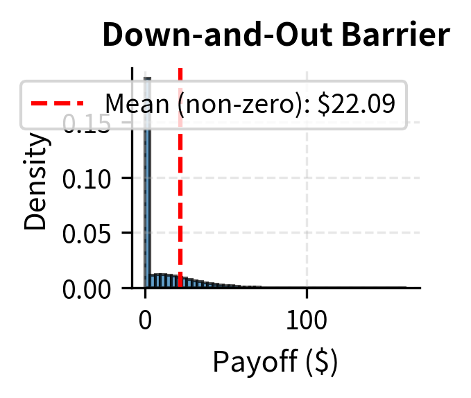
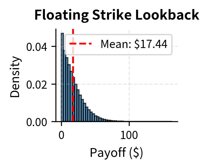
Notice the distinctive shapes: the Asian option has a compressed distribution due to averaging, the barrier option shows a large mass at zero from knocked-out paths, and the lookback option has a strictly positive distribution starting above zero.
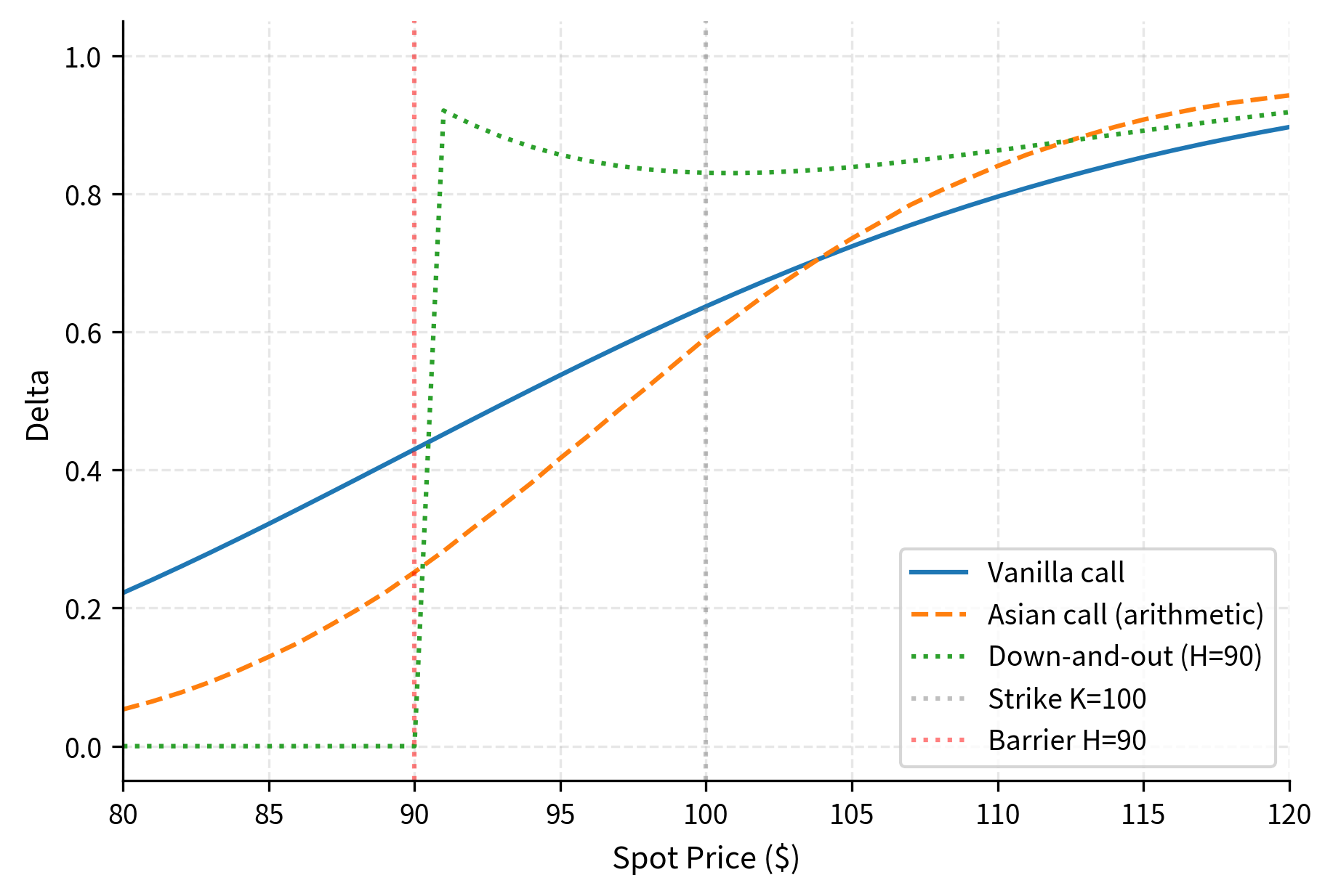
Greeks for Exotic Options
Risk management for exotic options requires computing the Greeks, as with vanilla options. However, path dependence and discontinuities in exotics create additional complexity.
Finite Difference Greeks
The simplest approach for computing Greeks uses finite differences. We bump inputs and reprice to estimate sensitivities:
where:
- : option price for spot price
- : current spot price
- : small change in price (bump size)
The central difference formula for delta provides second-order accuracy, meaning the error decreases quadratically as the bump size shrinks. The choice of bump size involves a trade-off: too large a bump introduces truncation error from ignoring higher-order terms, while too small a bump amplifies numerical noise in the price calculation. For Monte Carlo prices with inherent simulation noise, bump sizes of around 1% of the spot price typically work well.
The gamma formula uses a symmetric second difference, which also achieves second-order accuracy. However, gamma is inherently more difficult to estimate than delta because it involves the second derivative of price with respect to spot. Small errors in the individual price calculations become magnified when taking differences of differences, making gamma estimates noisier than delta estimates for the same computational effort.
For Monte Carlo pricing, this approach requires new sets of random paths for each bump, which can be computationally expensive and introduces noise.
Pathwise Greeks
A more efficient approach reuses the same random numbers across bumped prices. For path-dependent options with smooth payoffs, we can compute delta as:
where:
- : risk-free rate
- : time to expiration
- : expectation under the risk-neutral measure
- : sensitivity of the specific path's payoff to the initial price
This pathwise approach, sometimes called infinitesimal perturbation analysis, exploits the fact that we can often differentiate through the payoff function. For an Asian call with arithmetic average, the payoff is where . Each price on the path scales proportionally with the initial price , so . When the option finishes in the money, the derivative of the payoff with respect to is simply , the average price divided by the initial price.
The pathwise method fails when the payoff function is not differentiable, such as at the exercise boundary for options or at the barrier for barrier options. In these cases, the likelihood ratio method provides an alternative approach that differentiates the probability distribution rather than the payoff.
The calculated Greeks show a delta of 0.44, indicating the option is roughly at-the-money (ATM options typically have deltas near 0.5). The gamma of 0.0135 is notably lower than a vanilla ATM call's gamma, which would be around 0.020 for these parameters. This reduction occurs because averaging dampens the option's sensitivity to spot price changes: a single large price movement has less impact when it's averaged with many other observations. Similarly, the vega of $0.167 per 1% volatility is about 30% lower than a comparable vanilla call. The averaging mechanism reduces the option's exposure to volatility since what matters is the average volatility realized over many observations, not volatility at a single point in time. These lower Greeks make Asian options easier to hedge dynamically than their vanilla counterparts.
Practical Applications of Exotic Options
Exotic options serve specific purposes in financial markets that vanilla options cannot efficiently address.
Hedging with Asian Options
Consider a mining company that produces and sells gold throughout the year. The company's realized revenue depends on the average gold price over the year rather than the price on any single day. A strip of vanilla monthly options would be expensive and less precise. An Asian put option with payoff (where is the average gold price over 12 months) provides a direct hedge against their average revenue exposure.
Cost Reduction with Barrier Options
An investor bullish on a stock might buy an up-and-out call to reduce premium costs. If the stock rises significantly past the barrier, you lose the option but have already profited from holding the underlying. The barrier feature effectively caps the upside, which you are willing to accept in exchange for the lower premium.
Installment Options as Compound Options
A call on call can be structured as an installment option where the buyer pays a small initial premium for the right to pay a second premium later to acquire the full option. This is valuable when the buyer faces uncertainty about whether they'll need the hedge.
Limitations and Practical Considerations
Exotic options present several challenges beyond those encountered with vanilla options.
The first major concern is model risk. Exotic option prices are highly sensitive to model assumptions. While vanilla European options under Black-Scholes depend only on volatility and the model-free inputs (spot price, strike, time to expiration, interest rate), path-dependent exotics depend on the entire dynamics of volatility over the option's lifetime. A lookback option's price depends heavily on how volatility evolves over time, not just its average level. Constant volatility models can substantially misprice options when volatility is stochastic. In practice, traders often use local volatility or stochastic volatility models to more accurately capture the dynamics, though calibration becomes more complex. Subsequent chapters on volatility modeling cover these advanced approaches.
Barrier options introduce particular hedging difficulties. Near the barrier, delta and gamma become extremely large as the option value can swing from significant to zero with a small price movement. The discrete monitoring of barriers in practice, typically daily closes rather than continuous, creates basis risk between the theoretical and actual barrier observations. Dealers apply "barrier shift" adjustments to account for discrete monitoring. Additionally, in markets with jumps or overnight gaps, the barrier might be breached between monitoring times, creating model specification issues.
Liquidity is another practical concern. While vanilla options trade on exchanges with tight bid-ask spreads, most exotic options are traded over-the-counter. The bid-ask spreads for exotics can be five to ten times wider than for comparable vanilla options, reflecting the dealer's hedging costs and model risk. Unwinding an exotic position before maturity may be expensive or impossible if the original dealer is not willing to quote a price.
Path-dependent options require careful scenario analysis. Unlike vanilla options where the terminal price distribution suffices for risk analysis, path-dependent exotics require simulation of entire price paths. Value-at-Risk calculations must account for how the path taken affects the final payoff, not just the distribution of terminal prices.
Finally, counterparty credit risk becomes more significant for long-dated exotics. A 5-year lookback option accumulates significant value over time as the minimum price is tracked. If the option seller defaults before expiration, the buyer loses this accumulated value. Credit valuation adjustments (CVA) are particularly important for pricing long-dated exotic structures.
Summary
Exotic options extend the basic option framework to create instruments tailored to specific risk management needs and market views. The key concepts covered in this chapter include:
Path-dependent options have payoffs that depend on the price trajectory, not just the terminal value.
- Asian options use averages, reducing manipulation risk and matching hedging needs for average exposures.
- Barrier options knock in or out at specified levels, reducing premium but adding path contingency.
- Lookback options capture extrema, eliminating timing risk and commanding high premiums.
Non-path-dependent exotics include digital options with discontinuous payoffs and compound options (options on options).
Pricing approaches vary by option type.
- Some exotics admit closed-form solutions: geometric Asian, simple barriers, and digital options.
- Arithmetic Asian options require numerical methods or approximations.
- Monte Carlo simulation provides flexibility for complex path dependencies.
- Control variates using geometric Asian prices can accelerate arithmetic Asian pricing.
Risk management considerations for exotics include model dependence beyond vanilla options, hedging difficulties near barriers and at short maturities for digitals, and the need for scenario analysis that accounts for path dependence.
The numerical techniques we've developed throughout this part, particularly Monte Carlo methods with variance reduction and finite difference approaches, provide the computational backbone for pricing and risk-managing exotic derivatives. Subsequent chapters on interest rate models show how these exotic features, including barriers, averages, and lookbacks, appear in interest rate derivatives with additional complexity from the term structure dynamics.
Key Parameters
Key parameters for exotic options vary by type.
Asian Options:
- S₀: Current stock price. Higher prices increase call option values.
- K: Strike price. Determines the threshold for in-the-money payoff.
- T: Time to expiration. Longer durations increase option value.
- r: Risk-free rate. Affects discounting of expected payoff.
- σ: Volatility. Higher volatility increases option value.
- Average type: Arithmetic or geometric. Arithmetic averages lead to higher option values.
- n: Number of averaging points. More frequent averaging reduces sensitivity to extreme values.
Barrier Options:
- S₀: Current stock price. Starting point for the price path.
- K: Strike price. Determines payoff if option survives.
- H: Barrier level. The price that triggers knockout or knock-in.
- T: Time to expiration. Longer periods increase barrier-crossing probability.
- r: Risk-free rate. Affects both drift and discounting.
- σ: Volatility. Higher volatility increases probability of hitting barriers.
- Barrier type: Down-and-out, up-and-out, down-and-in, or up-and-in.
Lookback Options:
- S₀: Current stock price. Starting point for tracking extrema.
- Sₘᵢₙ or Sₘₐₓ: Historical minimum or maximum, relevant for options with existing history.
- T: Time to expiration. Longer periods increase likelihood of larger extrema.
- r: Risk-free rate. Affects discounting and drift.
- σ: Volatility. Higher volatility increases value significantly for lookback options.
- Strike type: Floating or fixed. This determines whether the strike or payoff reference changes.
Digital Options:
- S₀: Current stock price. Determines probability of finishing in-the-money.
- K: Strike price. The threshold for the discontinuous payoff.
- Q: Cash payout amount for cash-or-nothing digitals.
- T: Time to expiration. Affects probability calculations.
- r: Risk-free rate. Used for discounting.
- σ: Volatility. Affects the probability of crossing the strike.
Compound Options:
- S₀: Current stock price. Affects both compound and underlying option values.
- K₁: Strike of the compound option (cost to acquire the underlying).
- K₂: Strike of the underlying option.
- T₁: Expiration of the compound option.
- T₂: Expiration of the underlying option (must be > T₁).
- r: Risk-free rate. Affects both stages of the option.
- σ: Volatility. Impacts both decision points.
Quiz
Ready to test your understanding? Take this quick quiz to reinforce what you've learned about exotic options and complex derivatives.

Comments