

Learn binomial tree option pricing with the Cox-Ross-Rubinstein model. Price American and European options using backward induction and risk-neutral valuation.
Choose your expertise level to adjust how many terms are explained. Beginners see more tooltips, experts see fewer to maintain reading flow. Hover over underlined terms for instant definitions.
Binomial Tree Option Pricing
The Black-Scholes formula, which we derived in previous chapters, provides elegant closed-form solutions for European options. But what happens when you need to price an American put option, where early exercise might be optimal? Or an option with path-dependent features? The continuous-time framework becomes analytically intractable, and we need alternative approaches.
The binomial tree model, introduced by Cox, Ross, and Rubinstein in 1979, offers a powerful discrete-time alternative. Rather than assuming stock prices follow continuous geometric Brownian motion, the binomial model discretizes time into steps and assumes the stock price can only move up or down by fixed amounts at each step. This simplification makes the model remarkably tractable: you can price options by working backward through a tree of possible price paths, checking at each node whether early exercise is beneficial.
What makes binomial trees particularly valuable is that they're not just a pedagogical simplification. As you increase the number of time steps, the binomial model converges to Black-Scholes, providing both intuition for continuous-time results and a practical computational method for options that lack closed-form solutions. This chapter builds the binomial framework from first principles, shows how risk-neutral valuation applies at each node, and demonstrates pricing for both European and American options.
The One-Step Binomial Model
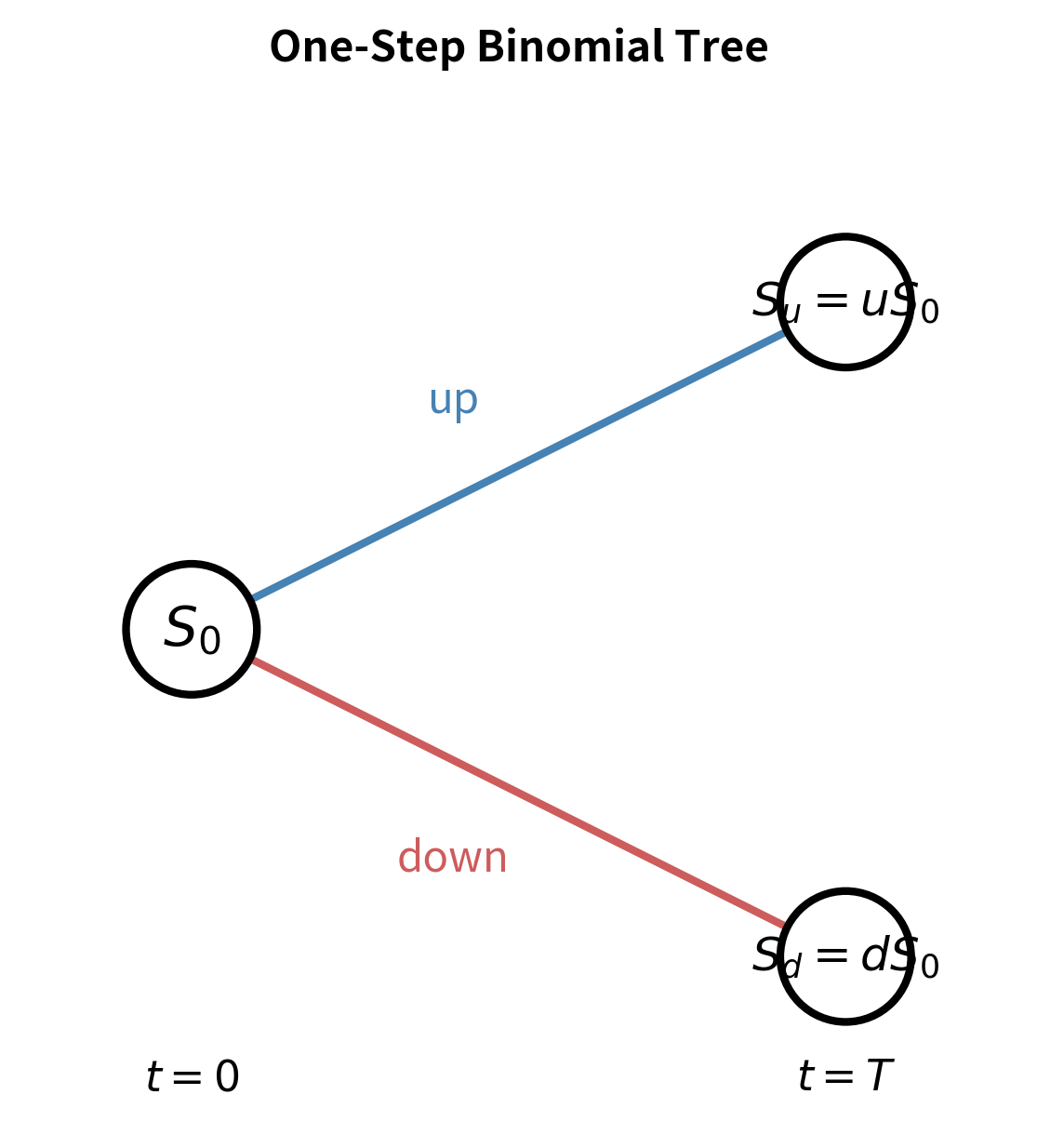
We begin with the simplest possible case: a single time step. This minimal setup strips away all complexity and reveals the core logic of option pricing in its purest form. By understanding how to price a derivative when there are only two possible future states of the world, we establish a foundation that extends seamlessly to models with thousands of time steps.
Consider a stock with current price that, after one period, will either move up to or down to , where and are the up and down factors. The up factor exceeds one because an "up" move represents an increase in price, while the down factor falls below one because a "down" move represents a decrease. We want to price a derivative with payoff if the stock goes up and if it goes down. Notice that we have not specified the probability of an up move. This omission is intentional and, as we shall see, reflects a key insight in derivative pricing: the option price does not depend on the probability of the stock rising.
Replicating Portfolio Approach
The key insight that unlocks option pricing in this framework is replication. Rather than trying to guess the probability of the stock going up or down, we construct a portfolio of basic assets whose payoff exactly matches the derivative's payoff in every possible future state. This replicating portfolio consists of two components: the underlying stock and a risk-free bond. If we can perfectly replicate the derivative using these tradeable instruments, then the derivative must have the same price as the portfolio, otherwise arbitrage opportunities would exist.
Suppose we hold shares of stock and invest dollars in a risk-free bond earning rate over the period. The parameter represents the number of shares we hold, which can be fractional, and represents our cash position in the risk-free bond, which can be positive (lending) or negative (borrowing). At expiration, after one time period , this portfolio is worth:
- Up state:
- Down state:
For this portfolio to replicate the derivative, we need:
where:
- : number of shares of stock in the portfolio
- : current stock price
- : up and down movement factors
- : amount invested in the risk-free bond
- : risk-free interest rate
- : time to expiration
- : option payoffs in the up and down states
This is a system of two linear equations in two unknowns ( and ). We can solve this system using straightforward algebraic manipulation. The strategy is to first eliminate one variable to find the other, then substitute back to complete the solution.
Subtracting the second equation from the first eliminates , since the bond value appears identically in both equations:
where:
- : number of shares in the portfolio
- : current stock price
- : up and down movement factors
- : bond investment
- : risk-free rate
- : time to expiration
- : option payoffs
This gives us the hedge ratio, which represents the number of shares needed to replicate the derivative:
where:
- : the hedge ratio (number of shares to hold)
- : the range of option payoffs
- : stock prices in up and down states
- : the range of stock prices
- : current stock price
- : up and down movement factors
This formula has a beautiful interpretation: the hedge ratio equals the change in option value divided by the change in stock price. This is exactly the discrete-time analog of the delta we encountered in continuous-time option pricing. It tells us how many shares to hold to hedge the derivative, and it measures the sensitivity of the option price to movements in the underlying stock. For a call option, is positive because the option gains value when the stock rises. For a put option, is negative because the option loses value when the stock rises.
Once we know , we can solve for by substituting back into either of our original equations. Using the up-state equation:
where:
- : present value of the bond investment
- : discount factor
- : portfolio cash needed to match the payoff in the up state
- : option payoffs
- : hedge ratio
- : up and down factors
- : current stock price
- : risk-free interest rate
- : time to expiration
The bond position is typically negative for call options, meaning we borrow money to fund the stock purchase. For put options, is typically positive, meaning we lend money while shorting stock.
No-Arbitrage Pricing
Since the replicating portfolio has the same payoff as the derivative in both states, by the no-arbitrage principle from Part III Chapter 4, the derivative must have the same price as the portfolio:
where:
- : current option price
- : number of shares held in the replicating portfolio
- : current stock price
- : value of the risk-free bond investment
If the derivative traded at any other price, an arbitrage opportunity would exist. If the derivative were cheaper than the replicating portfolio, we could buy the derivative, sell the portfolio, and pocket the difference while having perfectly offsetting positions. Conversely, if the derivative were more expensive, we could sell the derivative, buy the portfolio, and again lock in a risk-free profit. Market forces ensure that such opportunities are quickly eliminated, establishing the pricing relationship above.
Now we can derive an explicit formula for the option price by substituting our expressions for and into the portfolio value equation :
where:
- : current option price
- : number of shares held in the replicating portfolio
- : current stock price
- : weight assigned to the up payoff
- : weight assigned to the down payoff
- : risk-free interest rate
- : time to expiration
- : up and down factors
- : option payoffs
This final expression is remarkable: the option price is a discounted weighted average of the two possible payoffs. The weights depend only on the up and down factors and the risk-free rate, not on any probability of the stock going up or down. This observation leads us to one of the most important concepts in derivative pricing.
The Risk-Neutral Probability
The formula above has a beautiful interpretation. Define the risk-neutral probability :
where:
- : risk-neutral probability of an up move
- : up and down factors
- : risk-free rate
- : time step
Then the pricing formula becomes:
where:
- : current option price
- : risk-neutral probability
- : probability of a down move
- : risk-free discount factor
- : option payoffs in up and down states
- : risk-free interest rate
- : time step duration
This elegant formula states that the derivative price equals the discounted expected payoff, where the expectation uses the probability rather than the real-world probability of an up move. The expression computes the expected payoff under the risk-neutral probability measure, and the factor discounts this expected value back to the present. We never needed to know or estimate the actual probability of the stock rising; the risk-neutral probability emerges naturally from the no-arbitrage requirement.
The risk-neutral probability is not the actual probability of the stock going up. It's a mathematical construct that makes the expected return on the stock equal to the risk-free rate. Under this probability measure, the expected stock price is .
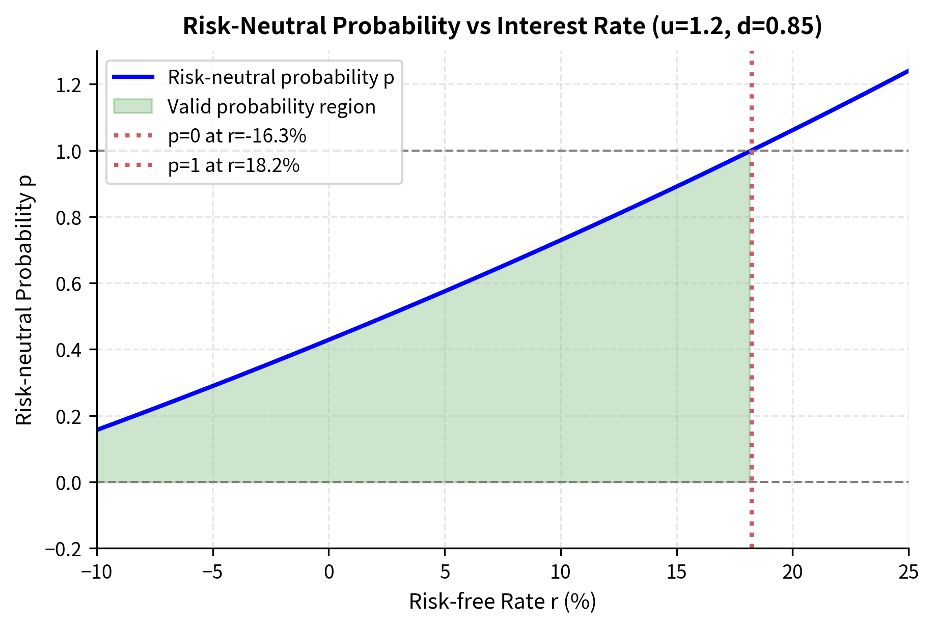
For to be a valid probability (between 0 and 1), we need:
where:
- : down movement factor
- : up movement factor
- : risk-free interest rate
- : time step duration
This condition ensures no arbitrage and has an intuitive economic interpretation. The term represents the growth factor of a risk-free investment over the period. The condition states that this risk-free growth must fall strictly between the down move and the up move . If , the risk-free bond would always outperform the stock, making the stock unattractive at any positive price. Conversely, if , the stock would always outperform the risk-free bond, meaning investors would borrow at the risk-free rate and invest in the stock for guaranteed profit. Either case would create an arbitrage opportunity, which cannot persist in equilibrium.
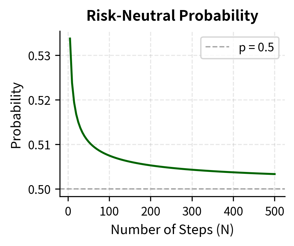
The calculated risk-neutral probability is close to 0.5 because with and , the up and down moves are roughly symmetric around the forward price . The forward price represents where the stock "should" be in the risk-neutral world, and when up and down moves are symmetric around this level, the risk-neutral probabilities are approximately equal.
Multi-Step Binomial Trees
The one-step model captures the essential logic, but real options require finer granularity. A single period cannot adequately represent the continuous evolution of stock prices over months or years. Moreover, for American options where early exercise is possible, we need intermediate time points to evaluate exercise decisions. We extend to multiple steps by dividing time to expiration into equal intervals, each of length . At each step, the stock price moves up by factor or down by factor , creating a tree of possible price paths.
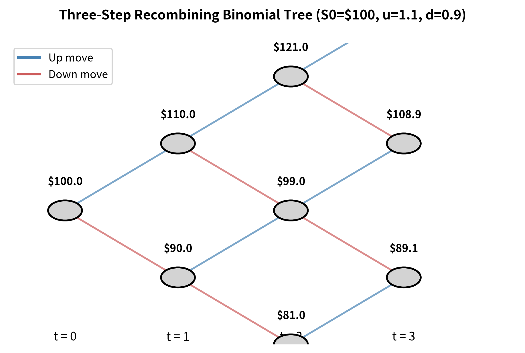
Tree Structure and Recombination
A crucial property of binomial trees is recombination: an up move followed by a down move leads to the same price as a down move followed by an up move (). This property arises because multiplication is commutative, so the order of multiplying by and does not matter. The recombination property dramatically reduces the computational burden of the tree. Without recombination, each node would branch into two new nodes, creating terminal nodes after steps. With recombination, the tree "collapses" as paths converge to common nodes, leaving only distinct prices at the final step.
At the final time step , the possible stock prices are:
where:
- : stock price at maturity node
- : initial stock price
- : up and down factors
- : total number of steps
- : number of up moves
The price corresponds to a node that can be reached by any path with exactly up moves and down moves. The number of paths reaching this node is given by the binomial coefficient , which counts the number of ways to arrange up moves among total moves. This combinatorial structure gives the model its name: the binomial tree.
Backward Induction
We price options by working backward through the tree, a technique known as backward induction. This approach exploits the fact that at maturity, option values are known with certainty since they equal the payoff function evaluated at each terminal stock price. Starting from the known payoffs at expiration and moving step-by-step toward time zero, we apply the one-step pricing formula at each node. At each step, we treat each node as if it were the root of a one-step tree and calculate the option value using the risk-neutral pricing formula derived earlier.
At the final step , the option value at node is simply the payoff:
where:
- : option value at maturity node
- : stock price at maturity node
- : strike price
These terminal values serve as the boundary conditions for our backward recursion. From these known values, we can calculate the option value at any node one step earlier.
For any earlier node at step with up moves, we compute the option value as:
where:
- : option value at step , node
- : time step size
- : risk-neutral probability
- : option value in the up state (next step)
- : option value in the down state (next step)
- : risk-free interest rate
This formula says that the option value at node equals the discounted risk-neutral expected value of the option at the next time step. If the stock moves up from node , it arrives at node ; if it moves down, it arrives at node . The recursion propagates backward until we reach node , which gives us the current option price.
Notice how the price oscillates and gradually converges as we increase the number of steps. This oscillatory behavior is characteristic of the binomial model and arises from the discrete nature of the tree structure. We'll explore this convergence behavior in detail later.
The Cox-Ross-Rubinstein Model
The choice of up and down factors and determines how well the discrete model approximates continuous-time dynamics. These parameters are not arbitrary; they must be chosen carefully to ensure that the discrete binomial process converges to the continuous geometric Brownian motion as the number of steps increases. The Cox-Ross-Rubinstein (CRR) parameterization, introduced in their seminal 1979 paper, sets:
where:
- : up and down factors
- : annualized volatility
- : time step size ()
The relationship ensures that the tree recombines: an up move followed by a down move returns the stock to its original price (). The exponential form reflects the multiplicative nature of stock returns, and the dependence on ensures that the volatility of the discrete model matches the volatility of the continuous model.
Derivation of CRR Parameters
The CRR parameters are chosen to match the first two moments of the log-return distribution under the continuous-time model. This moment-matching approach ensures that the discrete model faithfully reproduces the statistical properties of the continuous model it approximates.
In continuous time, over a small interval , the log-return has:
- Mean:
- Variance:
The mean reflects the drift of the log-price process, which under the risk-neutral measure equals the risk-free rate minus a convexity adjustment. The variance reflects the accumulated randomness over the time interval and grows proportionally with time.
In the binomial model, the log-return is either (with probability ) or (with probability ). These are the only two possible outcomes in the discrete model. The variance of this discrete log-return is:
where:
- : stock prices at time and
- : variance of a Bernoulli variable
- : difference in log prices between up and down states
- : magnitude of the log price jump
- : risk-neutral probability
- : volatility
- : time step
- : up and down factors
With the CRR choice and as , we can approximate the risk-neutral probability using Taylor series expansions. This analysis reveals how the probability approaches a specific limiting value:
where:
- : risk-neutral probability
- : up and down factors
- : drift adjustment term
- : time step size
- : scaling factor for the drift
- : risk-free interest rate
- : volatility
This derivation reveals that the risk-neutral probability approaches 1/2 as the time step shrinks, with a small correction proportional to . The correction term involves the drift rate , which is the expected growth rate of the log-price under the risk-neutral measure. This means as , giving variance , which matches the continuous-time variance.
Alternative Parameterizations
Other parameterizations exist with different properties:
-
Jarrow-Rudd (JR): Sets exactly and adjusts and to match moments. This gives equal probabilities but asymmetric up/down moves.
-
Tian: Matches the first three moments of the price distribution, potentially providing faster convergence.
For most practical purposes, the CRR parameterization works well and has become the standard choice. Its mathematical elegance, intuitive interpretation, and proven convergence properties make it the preferred approach in both academic and industry applications.
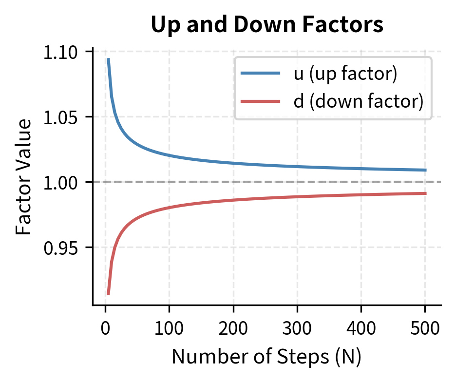
As increases (and decreases), the up and down factors approach 1, meaning each step represents a smaller price change. The risk-neutral probability approaches 0.5 plus a small drift adjustment, consistent with our theoretical analysis above.
Pricing American Options
The real power of binomial trees emerges when pricing American options, which can be exercised at any time before expiration. Unlike European options, American options have no known closed-form solution except in special cases (American calls on non-dividend-paying stocks are never optimally exercised early and thus equal European calls). The ability to exercise early adds a layer of complexity that continuous-time methods handle poorly, but binomial trees address naturally through backward induction.
Early Exercise Decision
At each node in the tree, you face a choice: exercise now or continue holding. The optimal strategy is to exercise if and only if the immediate exercise value exceeds the continuation value:
where:
- : American option value at node
- : immediate payoff from exercising the option
- : discounted expected value of holding the option
This simple modification to the backward induction algorithm transforms the European pricing method into an American pricing method. At each node, rather than automatically using the continuation value as we would for a European option, we compare it to the immediate exercise value and take the larger of the two.
For an American put at node :
where:
- : immediate exercise value (intrinsic value)
- : continuation value (discounted expected future value)
- : risk-neutral probability
- : option value at node
- : strike price
- : stock price at node
- : risk-free interest rate
- : time step
The first term is the immediate payoff from exercising; the second is the discounted expected value from waiting. By evaluating this comparison at every node, the algorithm finds the optimal exercise strategy and the corresponding option value.
Why American Puts May Be Exercised Early
For American puts, early exercise can be optimal when the stock price is sufficiently low. Consider a deep in-the-money put with strike $100 and stock price $10. Exercising immediately gives $90. Waiting means:
- You tie up $90 of potential proceeds
- The maximum additional gain is $10 (if the stock goes to zero)
- You risk the stock rising, reducing your payoff
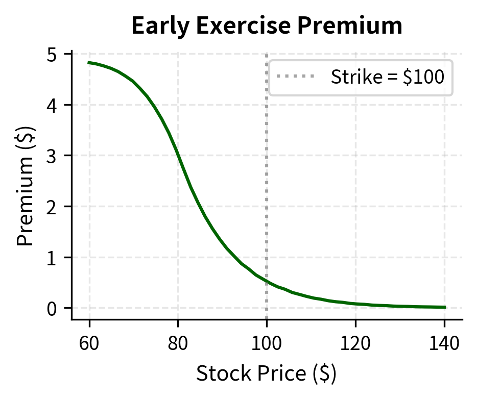
When the time value of money on the exercise proceeds exceeds the expected gain from waiting, early exercise is optimal. The $90 in immediate cash can be invested at the risk-free rate, earning interest. Meanwhile, the probability that the stock falls further to provide additional gains may be low, and the risk that it rises is significant. This trade-off creates a critical stock price below which early exercise is optimal, known as the early exercise boundary.
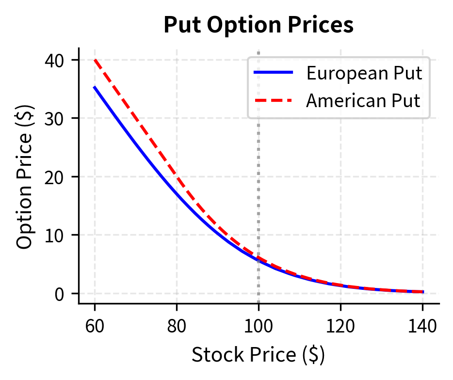
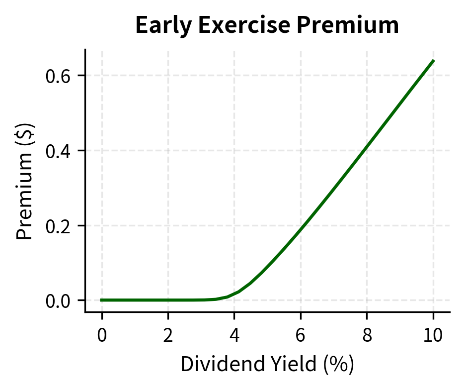
The American put is worth more than the European put because you have the valuable option to exercise early. This difference is called the early exercise premium and it represents the economic value of the flexibility to choose when to exercise.
Visualizing Early Exercise Regions
We can examine where in the tree early exercise is optimal by using a small number of steps and visualizing the exercise boundary.
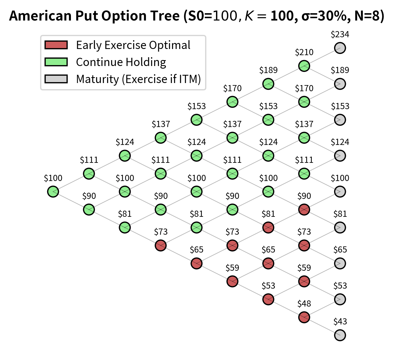
The early exercise boundary shows that for low stock prices (bottom of the tree), immediate exercise becomes optimal. This creates an "exercise region" below the boundary where you should exercise your puts. The boundary separates the state space into two regions: where it is optimal to continue holding the option and where it is optimal to exercise immediately.
Convergence to Black-Scholes
One of the most elegant properties of the binomial model is its convergence to the Black-Scholes price as the number of steps increases. This convergence is not merely a computational convenience; it provides theoretical validation that the binomial approach captures the same economic principles as the continuous-time framework. The convergence also offers practical assurance that binomial trees produce accurate prices when enough steps are used.
Theoretical Convergence
As we discussed in Part III Chapter 2, the binomial random walk converges in distribution to geometric Brownian motion as (a consequence of the central limit theorem applied to the sum of log-returns). Each step in the binomial tree contributes a small random increment to the log-price, and the sum of many such increments becomes normally distributed. Since the Black-Scholes model assumes geometric Brownian motion, and since both models use risk-neutral valuation, the binomial price converges to the Black-Scholes price.
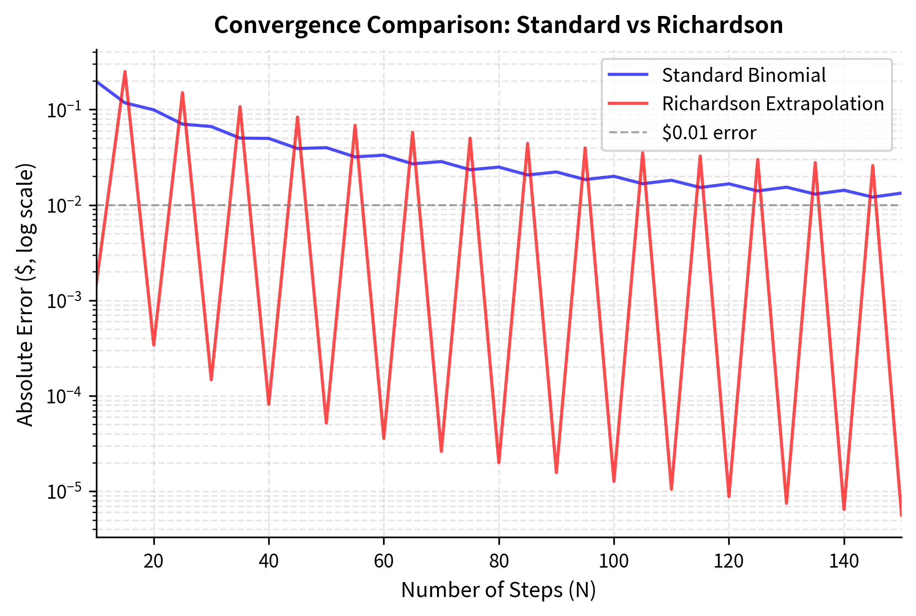
The rate of convergence for European options is , meaning doubling the number of steps roughly halves the error. However, convergence is not monotonic: prices oscillate around the true value, particularly for at-the-money options. This oscillation arises from the discrete nature of the tree and how the strike price falls relative to the tree's nodes at each step.
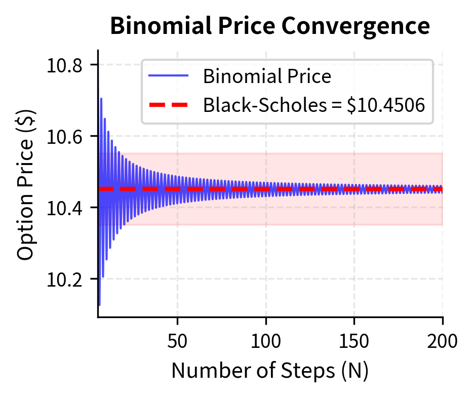
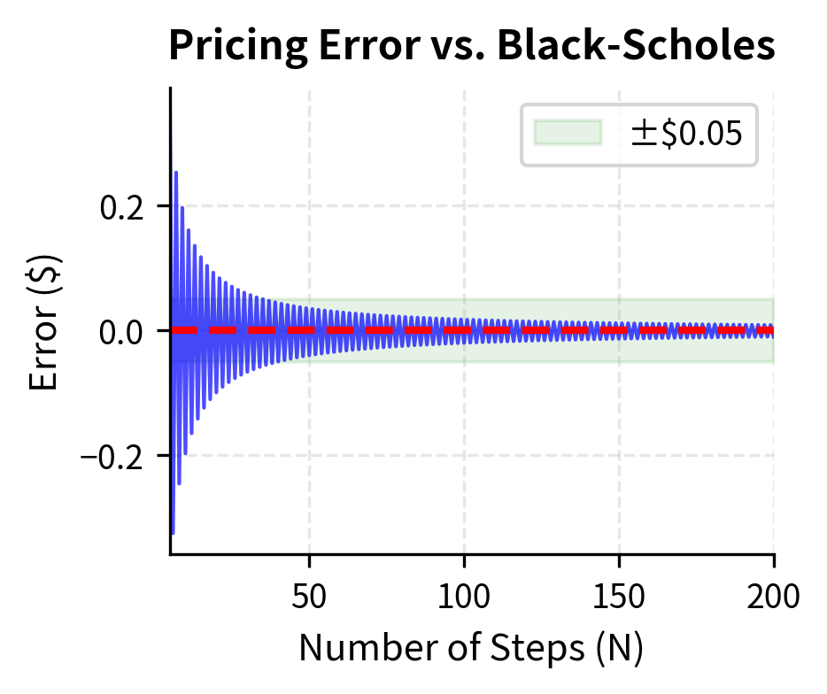
The characteristic oscillation occurs because of how the strike price falls relative to the tree's nodes. For even N, the strike may fall exactly on a node, while for odd N it falls between nodes. This creates alternating over- and under-estimation that damps out as N increases.
Convergence Rate Analysis
The error decreases roughly proportionally to :
The product being approximately constant confirms the convergence rate. This means that to reduce the error by a factor of 10, we need to increase the number of steps by a factor of 10, which has important implications for computational cost.
Complete Implementation
Let's build a more comprehensive implementation that includes visualization of the full tree and supports both European and American options.
The Greeks computed from the tree match the intuition from Part III Chapter 7: puts have negative delta (value decreases as stock rises), positive gamma (delta becomes less negative as stock rises), and negative theta (value decays over time).
Key Parameters
The key parameters for the Binomial Tree model are:
- S0: Current stock price. The starting node of the tree.
- K: Strike price. Used to calculate option payoffs at terminal nodes and exercise values for American options.
- T: Time to expiration in years. Determines the total duration covered by the tree.
- r: Risk-free interest rate (annualized). Used for discounting and calculating the risk-neutral probability.
- σ: Volatility (annualized). Determines the magnitude of up and down moves ( and ).
- N: Number of time steps. Controls the granularity of the tree; higher improves accuracy but increases computational cost.
- option_type: 'call' or 'put'. Determines the payoff structure.
- american: Boolean flag. If True, allows for early exercise checks at each node.
Dividends and Extensions
Real stocks often pay dividends, which affect option prices and early exercise decisions. The binomial framework easily accommodates dividends.
Continuous Dividend Yield
For stocks with a continuous dividend yield (common for index options), we modify the risk-neutral probability:
where:
- : risk-neutral probability adjusted for dividends
- : risk-free rate
- : continuous dividend yield
- : time step
- : up and down factors
The forward price grows at rate rather than , reflecting the dividend leakage. This modification accounts for the fact that holding the stock entitles you to dividends, which reduces the expected capital appreciation under the risk-neutral measure.
Discrete Dividends
For individual stocks paying discrete dividends, we adjust the stock price at dividend dates. If a dividend is paid at time , the stock price drops by immediately after payment. This creates a tree that is not strictly recombining around dividend dates but remains computationally tractable.
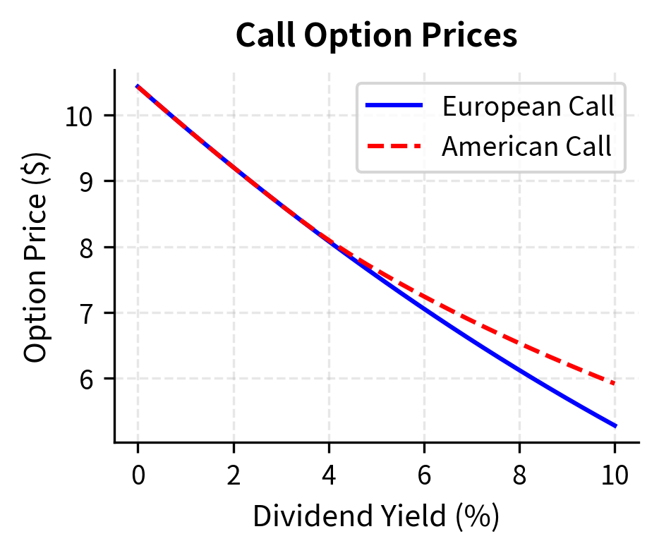
With no dividends, American calls equal European calls because early exercise is never optimal. As the dividend yield increases, early exercise becomes attractive: you want to own the stock to capture the dividend, making the American call more valuable than the European.
Practical Considerations and Limitations
While binomial trees are versatile and intuitive, several practical considerations arise when implementing them for production use.
Computational Complexity
The standard backward induction algorithm has time complexity because we process approximately nodes. For , this means roughly 500,000 node evaluations, which is fast on modern computers. However, for path-dependent options or trees with many underlying assets, complexity grows quickly.
Memory can be optimized by recognizing that we only need two adjacent columns at any time during backward induction. This reduces memory from to :
The negligible difference confirms that the memory-efficient implementation produces identical results to the standard approach, validating the optimization.
Oscillation and Convergence Enhancement
The oscillation in binomial prices can be problematic when high precision is needed. Several techniques improve convergence:
- Richardson extrapolation: Combine prices from N and 2N steps to cancel leading-order errors
- Smoothing: Average prices from N and N+1 steps
- Adaptive mesh: Place nodes exactly at the strike price
Richardson extrapolation significantly reduces the error for a given number of steps, making high-precision pricing computationally cheaper.
Limitations of Binomial Trees
Despite their flexibility, binomial trees have important limitations:
-
Single underlying asset: Standard trees handle one underlying. Multi-asset options require multi-dimensional trees where nodes grow exponentially with the number of assets.
-
Constant volatility: The basic model assumes constant volatility. For options with significant volatility smile effects, as we explored in Part III Chapter 8, extensions like implied trees are needed.
-
Path independence assumption: The recombining tree structure assumes the derivative's value depends only on the current stock price, not the path taken. Path-dependent options like Asian or lookback options require different approaches, which we'll explore in Part III Chapter 13 on exotic options.
-
Slow convergence for some payoffs: Options with discontinuous payoffs (like digital options) converge slowly because the discrete tree poorly approximates the discontinuity.
For options where binomial trees become cumbersome, Monte Carlo simulation (covered in the next chapter) and finite difference methods (Part III Chapter 12) offer powerful alternatives.
Summary
Binomial trees provide an intuitive and flexible framework for option pricing that bridges the gap between theoretical understanding and practical computation.
The key concepts from this chapter include:
-
Discrete-time modeling: Stock prices evolve through discrete up and down moves, with the Cox-Ross-Rubinstein parameterization and ensuring convergence to geometric Brownian motion.
-
Risk-neutral valuation: The risk-neutral probability allows pricing as a discounted expected payoff without knowing the true probability of up moves.
-
Backward induction: Option prices are computed by working backward from known terminal payoffs, applying the one-step pricing formula at each node.
-
American options: Early exercise is handled by comparing exercise value to continuation value at each node, making binomial trees the method of choice for American-style derivatives.
-
Convergence to Black-Scholes: As the number of steps increases, binomial prices converge to Black-Scholes at rate , with Richardson extrapolation improving accuracy.
The binomial framework extends naturally to dividend-paying stocks, exotic features, and serves as a foundation for understanding more advanced numerical methods. In the next chapter, we'll explore Monte Carlo simulation, which handles high-dimensional problems and path-dependent options that are challenging for tree-based methods.
Quiz
Ready to test your understanding? Take this quick quiz to reinforce what you've learned about binomial tree option pricing.

Comments