

Learn finite difference methods for option pricing. Master explicit, implicit, and Crank-Nicolson schemes to solve the Black-Scholes PDE numerically.
Choose your expertise level to adjust how many terms are explained. Beginners see more tooltips, experts see fewer to maintain reading flow. Hover over underlined terms for instant definitions.
Finite Difference Methods for Option Pricing
Derivative pricing uses two major numerical approaches: binomial trees, which discretize the underlying asset's price movements into up and down jumps, and Monte Carlo simulation, which generates random paths of the underlying asset to estimate option values. Both methods are powerful, but they approach the pricing problem from a probabilistic perspective, simulating possible futures and working backward or averaging outcomes.
Finite difference methods take an entirely different approach. Rather than simulating the stochastic process that drives asset prices, they directly attack the partial differential equation (PDE) that governs option values. As shown in the chapter on the Black-Scholes-Merton PDE, the option price satisfies a deterministic equation that can be solved numerically by discretizing both the asset price and time dimensions onto a grid.
This chapter develops three finite difference schemes, each representing a different trade-off between computational simplicity and numerical stability: the explicit scheme, the implicit scheme, and the Crank-Nicolson scheme. Understanding these methods provides essential tools for pricing options where analytical solutions don't exist, including American options with early exercise features and exotic derivatives with complex payoff structures. We'll examine how to set up the computational grid, handle boundary conditions, ensure numerical stability, and implement each scheme in practice.
The Black-Scholes PDE on a Grid
The foundation of finite difference methods is the Black-Scholes PDE, which is derived using Itô's lemma and the principle of no-arbitrage pricing. Recall that this partial differential equation emerges from the requirement that a perfectly hedged portfolio of an option and its underlying asset must earn the risk-free rate. The equation captures how the option value evolves as time passes and as the underlying asset price fluctuates. For an option with value on an underlying asset with price , the PDE is:
where:
- : option price as a function of asset price and time
- : risk-free interest rate
- : volatility of the underlying asset
- : diffusion term capturing the effect of volatility
- : drift term reflecting the risk-neutral expected return
- : discounting term reflecting the time value of money
Each term in this equation has a clear financial interpretation that helps us understand why the option value must satisfy this relationship. The time derivative captures how the option value changes purely due to the passage of time, with all else held constant. The second derivative term, sometimes called the gamma term, reflects the convexity of the option's payoff and how volatility affects value. When an option has positive gamma, increased volatility raises its expected payoff under risk-neutral pricing. The first derivative term represents the delta exposure, capturing how the option value responds to small changes in the underlying price. Finally, the discounting term ensures that the option value is expressed in present-value terms, consistent with no-arbitrage pricing. This equation, combined with appropriate boundary conditions and a terminal condition at expiration, uniquely determines the option value.
Transforming to a Standard Form
Working directly with the Black-Scholes PDE can be cumbersome because the coefficient in front of the second derivative varies with . This spatial dependence of the coefficients means that the diffusion rate changes across the price grid, which can complicate numerical analysis and introduce additional discretization challenges. A common transformation simplifies the problem by converting to log-price coordinates. The key insight is that if the stock price follows geometric Brownian motion, then the log of the stock price follows arithmetic Brownian motion with constant volatility. Let , so . After applying the chain rule to transform the derivatives:
where:
- : option value
- : asset price
- : log-price coordinate ()
The transformation of the first derivative follows directly from the chain rule. For the second derivative, we must apply the product rule and chain rule together, recognizing that itself depends on . The calculation yields:
where:
- : second derivative (gamma) in price coordinates
- : derivatives in log-price coordinates
Notice how the transformation introduces a correction term: the second derivative in log-coordinates does not simply equal times the second derivative in price coordinates. This correction arises because the log transformation is nonlinear, stretching the coordinate system differently at different price levels. Substituting these transformed derivatives into the Black-Scholes PDE and simplifying yields a much simpler equation:
where:
- : option value
- : time
- : volatility
- : risk-free rate
- : log-price coordinate
This transformed equation has constant coefficients, making it more amenable to finite difference approximations because the same discretization scheme applies uniformly across the entire spatial domain. The coefficient in front of the first derivative is the risk-neutral drift of the log-price process, which should be familiar from the study of the Black-Scholes-Merton model. To keep things clear and practical, we'll focus on the original -coordinate formulation. This makes setting boundary conditions and interpreting results more intuitive.
Setting Up the Computational Grid
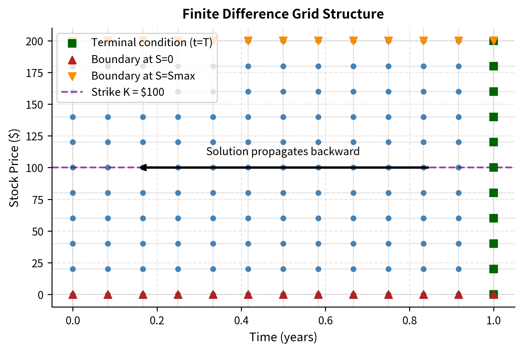
To solve the PDE numerically, we must replace the continuous price and time domains with discrete grid points. This process, called discretization, transforms the continuous partial differential equation into a system of algebraic equations that a computer can solve. For the asset price , we create a grid from to , where is chosen large enough that the option value is negligible for out-of-the-money options. For time, we work backward from expiration to the current time , which aligns with the natural direction for solving parabolic PDEs with terminal conditions.
The grid points are defined as:
- Price grid: for , where
- Time grid: for , where
Let denote the option value at grid point . This notation uses subscripts for spatial indices and superscripts for temporal indices, a convention that helps distinguish the two dimensions of the problem. Our goal is to compute the option values at (current time) given the terminal condition at (expiration). The backward-in-time solution process mirrors the logic of risk-neutral valuation: we know the option's payoff at expiration and work backward to determine its present value.
The choice of grid parameters involves trade-offs that you must carefully consider. Finer grids (larger and ) provide more accurate solutions but require more computation and memory. The grid must be fine enough to capture the option's behavior near the strike price, where values change most rapidly, but extending the grid too far into deep in-the-money or out-of-the-money regions wastes computational resources. The ratio between and is particularly important for stability, as we'll see when analyzing each scheme.
The Explicit Finite Difference Scheme
The explicit scheme is the most straightforward approach to solving the Black-Scholes PDE numerically. Its simplicity makes it an excellent starting point for understanding finite difference methods, even though its stability limitations often favor other schemes in practice. The explicit scheme approximates the PDE derivatives using values at the current time step to calculate values at the previous time step (remembering that we work backward from expiration).
Derivative Approximations
The central idea of finite difference methods is to replace derivatives with algebraic approximations involving function values at nearby grid points. These approximations come from Taylor series expansions. We approximate the partial derivatives using finite differences. At grid point , the approximations are:
Time derivative (backward difference):
where:
- : option value at grid point and current time step
- : option value at grid point and next time step
- : time step size
This approximation follows from the definition of a derivative as a limit. When we cannot take an infinitesimal step, we use a small but finite step instead. The error in this approximation is proportional to , meaning we achieve first-order accuracy in time.
First spatial derivative (central difference):
where:
- : option values at adjacent spatial points at time
- : price step size
The central difference uses function values on both sides of the point of interest, which leads to a symmetric approximation with second-order accuracy. Compared to one-sided differences, the central difference cancels the leading error terms, giving a more accurate estimate of the derivative.
Second spatial derivative (central difference):
where:
- : option values at adjacent spatial points
- : price step size
This formula for the second derivative can be derived by applying the first derivative approximation twice, or equivalently by using Taylor expansions and solving for the second derivative. The resulting expression has an intuitive interpretation: it measures the curvature of the option value function by comparing the value at a point to the average of its neighbors. Notice that all spatial derivatives use values at time . This makes the scheme "explicit" because we can directly calculate from known values at without needing to solve a system of equations.
Deriving the Update Formula
With our finite difference approximations in hand, we can now derive the explicit update formula by substituting into the Black-Scholes PDE. Substituting these approximations into the Black-Scholes PDE and rearranging for :
where:
- : unknown option value at current time step
- : known option values at next time step
- : asset price at grid point
- : time and price step sizes
- : risk-free rate and volatility
Our objective is to isolate on one side of the equation, expressing it in terms of known quantities. Multiplying by and rearranging to isolate :
where:
- : option value at the current time step
- : time step size
- Terms in parenthesis: discrete approximation of the Black-Scholes operator
The expression in parentheses represents the spatial part of the Black-Scholes operator, evaluated at the known time step. To make the formula more useful for computation, we collect terms by which grid point they involve. Grouping terms by the grid points , , and :
where:
- : option value at the current time step
- : time step size
- : price step size
- : volatility
- : risk-free rate
- : asset price at grid point
- : option values at the next time step
The structure of this equation reveals that the option value at any interior grid point is a weighted combination of three values at the next time step: the value at the same price level and the values at adjacent price levels. Using , these bracketed terms simplify to a more compact form:
where:
- : option value at the current time step
- : known option values at the next time step
- : weighting coefficients for the grid points
The coefficients are:
where:
- : time step size
- : volatility
- : risk-free rate
- : grid index ()
The option value at each interior point depends only on three values at the next time step, which we already know from either the terminal condition or previous calculations. Intuitively, this weighted sum resembles an expected value calculation: and represent the weights (pseudo-probabilities) of the asset price moving down or up, while is the weight of staying effectively in the same region, all adjusted for the risk-free discounting. This probabilistic interpretation connects finite difference methods to the binomial tree approach, where we also computed option values as discounted expected values under risk-neutral probabilities. The explicit scheme essentially implements the same logic on a finer grid.
Implementation
The explicit scheme proceeds as follows:
- Initialize the grid with the terminal payoff at expiration
- Apply boundary conditions at and
- Sweep backward through time, calculating each from values at
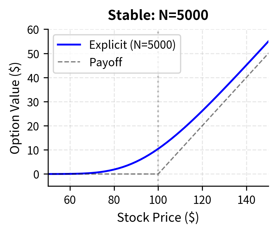
The calculated option price represents the fair value derived from the explicit finite difference grid. Since the grid is relatively fine (5000 time steps), this value closely approximates the theoretical Black-Scholes price, serving as a baseline for verifying the numerical method's accuracy.
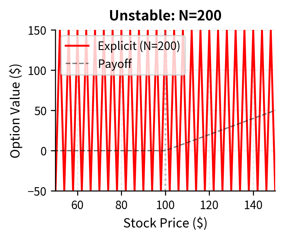
Stability Constraint
The explicit scheme has a critical limitation. It becomes unstable if the time step is too large. This instability arises because the coefficients must behave like probabilities to ensure the solution remains bounded. When we interpret these coefficients as weights in an expected value calculation, they should all be non-negative for the scheme to behave sensibly. If is too large, becomes negative, causing errors to oscillate and grow exponentially with each time step. Small numerical errors introduced by rounding or discretization get amplified rather than damped, eventually overwhelming the true solution. The stability condition requires:
where:
- : maximum allowable time step
- : volatility
- : risk-free rate
- : maximum grid index ()
In practice, this means:
where:
- : maximum stable time step
- : price grid spacing
- : volatility
- : maximum price on the grid
This constraint can be severe because the bound depends on the square of the price grid spacing. Halving to improve spatial resolution requires dividing by four to maintain stability. For typical parameters, the explicit scheme may require thousands of time steps to remain stable, making it computationally expensive despite its conceptual simplicity. This stability restriction motivates the development of implicit methods that remove or relax this constraint.
The stability requirement explains why we used 5,000 time steps in our implementation. Using fewer steps would cause the solution to oscillate wildly and diverge from the true option value.
The Implicit Finite Difference Scheme
The implicit scheme overcomes the stability limitation by evaluating the spatial derivatives at the current time step rather than the future time step . This small change significantly improves numerical stability. Rather than computing values at time directly from known values at , the implicit scheme requires solving for all values at simultaneously, since the update formula for each point involves unknown values at neighboring points at the same time level.
Derivative Approximations
The implicit scheme uses the same time derivative approximation as the explicit scheme but evaluates the spatial derivatives at a different time level. The implicit scheme uses:
Time derivative (backward difference):
where:
- : option value at grid point and current time step
- : option value at grid point and next time step
- : time step size
Spatial derivatives at time :
where:
- : option values at current time (unknowns)
- : price step size
The crucial distinction from the explicit scheme is that these spatial derivatives use values at time , which are the unknowns we seek to determine. This creates a coupling between neighboring grid points at the same time level: to find , we need and , but these values are also unknown.
The Tridiagonal System
Because all values at time are coupled together, we cannot compute them one at a time. Instead, we must solve a system of linear equations simultaneously. Substituting the approximations into the Black-Scholes PDE:
where:
- : unknown option values at current time
- : known option value at next time
We multiply by and isolate :
Grouping the unknown terms at by spatial index:
Defining coefficients to simplify notation, we obtain the linear system:
where:
- : unknown values at current time
- : known value at next time
- : coefficients for the implicit system
The coefficients are:
where:
- : time step
- : volatility
- : risk-free rate
- : spatial index corresponding to
Unlike the explicit scheme, we cannot directly calculate from . Instead, we must solve a system of linear equations at each time step. For the interior points, this forms a tridiagonal matrix equation:
where:
- : tridiagonal coefficient matrix
- : vector of option values at time (unknowns)
- : vector of known option values at time
- : vector incorporating boundary conditions
The Tridiagonal Matrix Structure
The matrix has the form:
where:
- : coefficients defined previously
- : number of spatial grid intervals
The tridiagonal structure arises because each interior equation involves only three unknowns: the value at the current grid point and its two immediate neighbors. This sparse structure is extremely important computationally because it allows efficient solution algorithms. By coupling all values in a single system, the implicit method allows information to propagate across the entire grid instantaneously, mirroring the infinite propagation speed of the diffusion equation. In contrast, the explicit scheme propagates information only one grid point per time step, which is why it requires the stability constraint. This global dependency ensures errors are damped rather than amplified, providing unconditional stability. Tridiagonal systems can be solved very efficiently using the Thomas algorithm (a specialized form of Gaussian elimination), requiring only operations per time step, making the implicit scheme practical even though it requires solving a linear system.
Implementation
The implicit method yields a price very close to the explicit method but achieves this using only 500 time steps, one-tenth of the effort required for the explicit scheme. This efficiency demonstrates the practical benefit of unconditional stability.
Unconditional Stability
The implicit scheme is unconditionally stable, meaning it produces bounded solutions for any choice of and . This property allows you to use much larger time steps, dramatically reducing computation. Although each time step requires solving a linear system, the overall efficiency often surpasses the explicit scheme because far fewer time steps are needed.
The stability comes from the implicit treatment of the spatial derivatives. Mathematically, when we analyze the amplification factor of the numerical scheme, the implicit treatment ensures that errors decay rather than grow over time. Any errors introduced in one time step are damped rather than amplified in subsequent steps. The price we pay for this stability is the need to solve a linear system at each time step, but for tridiagonal systems this cost is minimal.
The Crank-Nicolson Scheme
The Crank-Nicolson scheme represents a middle ground between explicit and implicit methods. It averages the spatial derivatives at times and , achieving second-order accuracy in time while maintaining unconditional stability. This combination of accuracy and stability makes Crank-Nicolson the method of choice for most practical applications.
The Averaging Approach
Instead of evaluating spatial derivatives entirely at (implicit) or (explicit), Crank-Nicolson uses the average of both evaluations. This averaging can be motivated by the trapezoidal rule for numerical integration: when integrating the time derivative, we approximate the integral of the spatial operator by averaging its values at the beginning and end of the time interval. The scheme uses:
where:
- : values at current time step
- : values at next time step
- : price step size
and similarly for the first derivative. This averaging can be viewed as taking a half-step with the explicit scheme and a half-step with the implicit scheme. The explicit part uses known information from the future time step, while the implicit part ensures stability by coupling values at the current time step.
The Discretized Equation
Substituting the approximations into the Black-Scholes PDE:
where:
- : spatial operator at node , equal to
- : option values at current and next time steps
The spatial operator encapsulates all the terms involving spatial derivatives and the discounting term. Applying this operator at both time levels and averaging creates the characteristic Crank-Nicolson structure. Rearranging terms by time step:
where:
- LHS: implicit terms at current time
- RHS: explicit terms at next time
- : Crank-Nicolson coefficients
The left side involves unknown values at , forming a tridiagonal system just as in the implicit scheme. The right side uses known values at , which we can compute explicitly before solving the system. The coefficients are:
where:
- : time step
- : volatility
- : risk-free rate
- : spatial index
Notice that these coefficients are exactly half of the corresponding implicit scheme coefficients, reflecting the averaging of the spatial operator between two time levels. The left side involves unknown values at , while the right side uses known values at . This again leads to a tridiagonal system at each time step.
Implementation
The Crank-Nicolson price is consistent with the other methods. By averaging the explicit and implicit approaches, it maintains stability while improving accuracy, effectively reducing the bias introduced by time discretization.
Accuracy Analysis
The Crank-Nicolson scheme achieves accuracy in time, compared to for both the explicit and implicit schemes. This means that halving the time step reduces the time discretization error by a factor of four rather than two. The improved accuracy comes from the averaging, which cancels the leading-order error terms in the Taylor expansion. For most applications, Crank-Nicolson provides the best balance of accuracy, stability, and computational efficiency.
Boundary Conditions
Proper boundary conditions are essential for finite difference methods. They determine the option value at the edges of the computational grid, where the standard update formulas cannot be applied directly because they would require values outside the grid.
Terminal Condition
At expiration (), the option value equals its payoff. This is the fundamental condition that initializes our backward-in-time computation:
where:
- : option value at expiration
- : stock price at expiration
- : strike price
This condition initializes the grid before we begin the backward time-stepping process. The non-smooth nature of the payoff function at can introduce complications, as the second derivative is undefined at that point. You might sometimes smooth the payoff near the strike to improve numerical behavior.
Boundary at
When the underlying asset price is zero, it remains at zero forever (assuming geometric Brownian motion). This follows because geometric Brownian motion has the property that zero is an absorbing state: if , then implies . Therefore:
-
where:
- : option value at asset price zero
(a call is worthless if the stock is worthless)
-
Put option:
where:
- : option value at asset price zero
- : strike price
- : risk-free interest rate
- : time to expiration
(a put pays at expiration with certainty)
Boundary at
At very high stock prices, we need to specify the option value at the upper edge of the grid. The exact value depends on the type of option:
-
Call option:
where:
- : option value at maximum grid price
- : maximum asset price on the grid
- : strike price
- : risk-free interest rate
- : time to expiration
(deep in-the-money, behaves like a forward)
-
Put option:
where:
- : option value at maximum grid price
(deep out-of-the-money)
The boundary at requires some care. If is chosen too small, the boundary condition may distort the solution in the region of interest. A rule of thumb is to set to for typical volatilities.
Implementing Put Option Boundaries
Convergence Analysis and Method Comparison
Now let's compare all three finite difference methods against the analytical Black-Scholes formula to assess their accuracy and convergence properties.
All three methods converge to the analytical Black-Scholes price. The Crank-Nicolson scheme achieves an error comparable to the implicit scheme in this snapshot, but with better theoretical convergence properties that become apparent on finer grids.
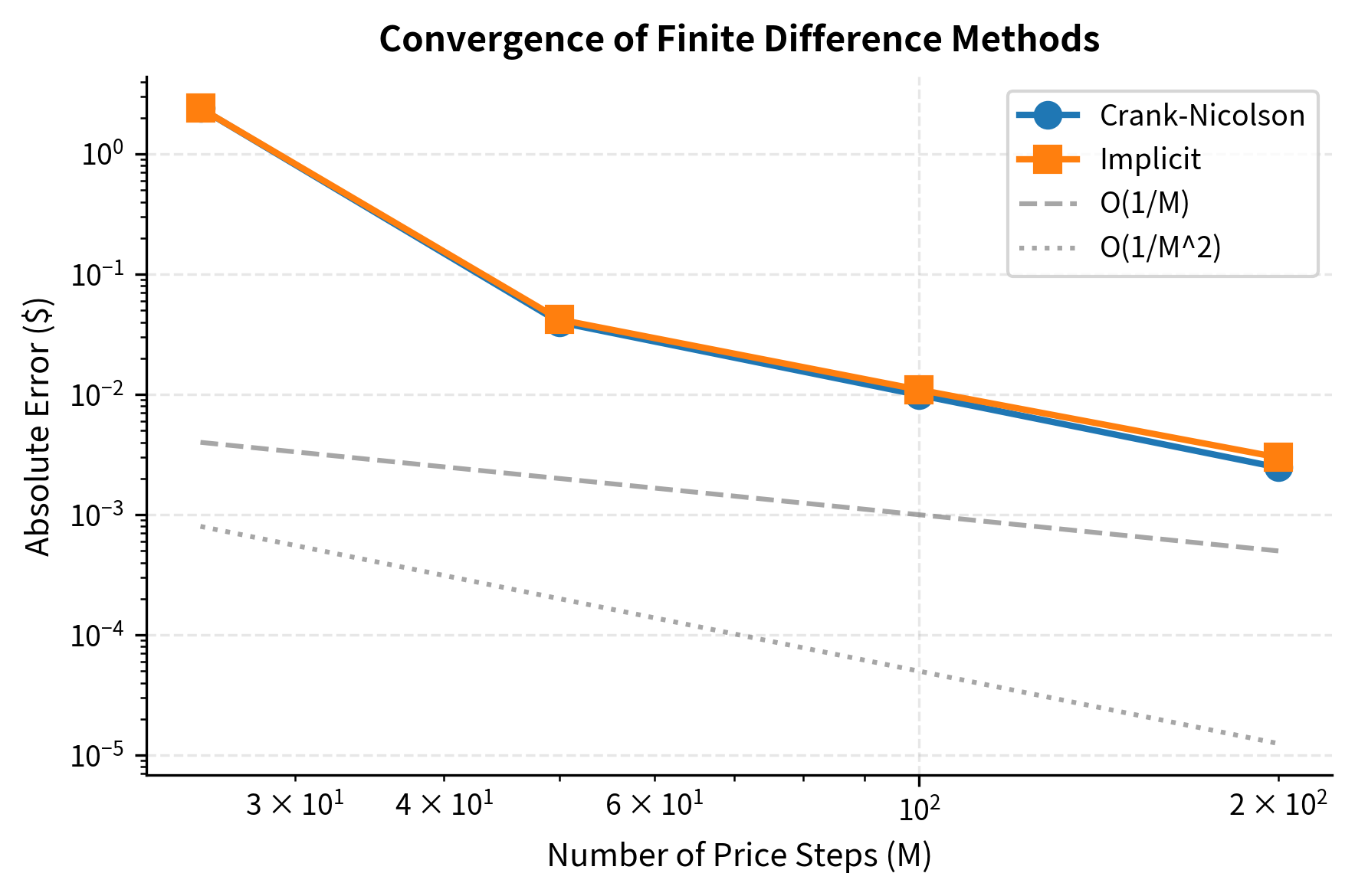
Convergence Study
Let's examine how the error decreases as we refine the grid. This reveals the order of convergence for each method.
The convergence plot reveals that both methods achieve approximately first-order convergence in the spatial discretization. Crank-Nicolson typically produces smaller absolute errors due to its superior time accuracy. The implicit scheme's errors are slightly larger but within the same order of magnitude.
Pricing American Options
American options are a major application for finite difference methods because they can be exercised at any time. The analytical Black-Scholes formula doesn't apply to American options, making numerical methods essential.
The Early Exercise Constraint
For an American option, at each point in time we must check whether early exercise is optimal. The key insight is that no rational holder would keep an option whose continuation value (the value if held) falls below its intrinsic value (the value if exercised immediately). The option value cannot fall below its intrinsic value:
where:
- : American option value
- : current stock price
- : strike price
In finite difference terms, after each backward time step, we apply:
where:
- : option continuation value computed by the FD scheme
- : immediate exercise value (e.g., for a put)
- : operator selecting the higher of holding or exercising
This simple modification converts our European option pricer into an American option pricer. This step implements the dynamic programming principle: at each state, we compare the value of waiting (continuation value) against the value of acting now (exercise value) and rationally choose the maximum. The finite difference framework handles this naturally because we solve backward in time, determining the optimal decision at each grid point given knowledge of future values.
Implementation
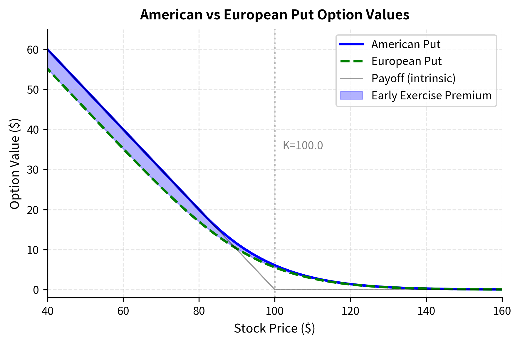
The early exercise premium represents the additional value an American put holder gains from the flexibility to exercise early. This premium is positive for puts on non-dividend-paying stocks because the put holder can capture the strike price immediately rather than waiting and earning interest on the proceeds.
Visualizing the Early Exercise Boundary
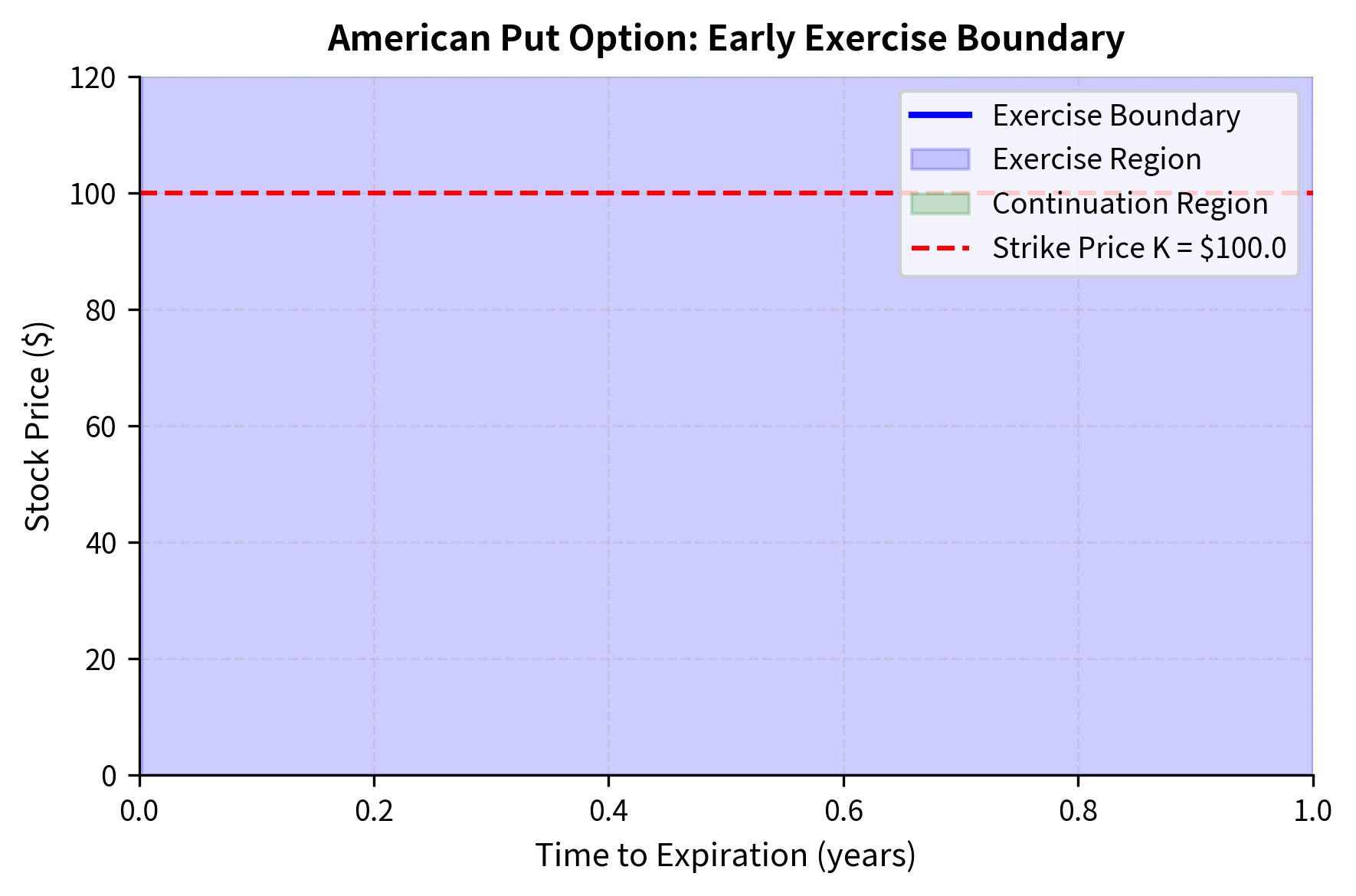
The early exercise boundary shows the critical stock price below which immediate exercise is optimal. As time to expiration decreases, this boundary rises toward the strike price because the time value of waiting diminishes.
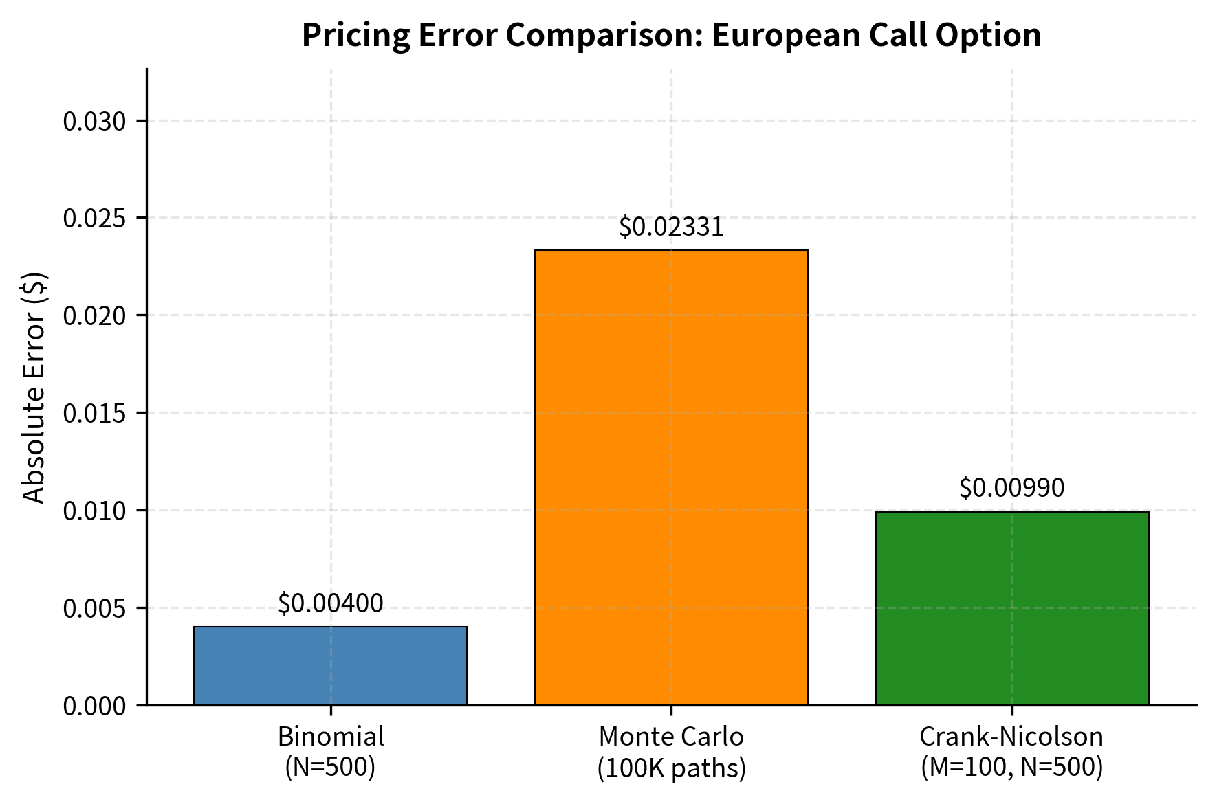
Comparing Methods: A Comprehensive View
Let's bring together all the numerical methods we've covered for pricing options: binomial trees, Monte Carlo simulation, and finite difference methods.
The Finite Difference (Crank-Nicolson) method matches the exact Black-Scholes price with high precision, comparable to the Binomial Tree. Unlike Monte Carlo, which shows stochastic variation, the finite difference result is deterministic and stable for this 1D problem.
Method Characteristics
Each numerical method has distinct strengths and weaknesses:
Binomial Trees:
- Intuitive, based on discrete price movements
- Natural for American options with early exercise
- Accuracy limited by number of time steps
- Convergence can be non-monotonic
- Excellent for path-dependent options
- Easily handles multiple underlying assets (high dimensions)
- Statistical error decreases slowly ()
- Less natural for American options (though methods like Longstaff-Schwartz exist)
Finite Difference Methods:
- Directly solves the pricing PDE
- Very efficient for one or two underlying assets
- Natural for American options and barrier options
- Difficulty increases rapidly with dimension
When to Use Each Method
The choice of numerical method depends on the specific option being priced:
- European options on single assets: All methods work well; analytical formulas (when available) are fastest
- American options: Finite difference methods and binomial trees are natural choices
- Barrier options: Finite difference methods handle absorbing boundaries elegantly
- Path-dependent options (Asian, lookback): Monte Carlo is typically preferred
- Multi-asset options: Monte Carlo scales better to high dimensions
We'll explore exotic options and their pricing in the next chapter, where we'll see how these numerical methods adapt to more complex payoff structures.
Key Parameters
The key parameters for finite difference option pricing are:
- S: Current stock price. Represents the underlying asset value at any grid point.
- K: Strike price. Determines the option payoff at expiration and intrinsic value.
- T: Time to expiration. The domain over which the PDE is solved.
- r: Risk-free interest rate. Used for drift in the PDE and discounting.
- : Volatility. Determines the diffusion coefficient in the Black-Scholes PDE.
- M: Number of price steps. Determines spatial resolution ().
- N: Number of time steps. Determines temporal resolution () and stability.
Practical Considerations
Implementing finite difference methods in practice requires attention to several technical details that affect both accuracy and computational performance.
Grid Design
The accuracy of finite difference solutions depends heavily on grid design. Key considerations include:
Price grid spacing: Finer grids near the strike price improve accuracy where option values change most rapidly. Non-uniform grids can concentrate points where they matter most.
Grid boundaries: should be large enough that the boundary condition is accurate. For deep out-of-the-money regions, the option value is near zero regardless of the exact boundary.
Time steps: Even unconditionally stable methods benefit from reasonable time step sizes. Too few steps introduce significant discretization error.
Computational Efficiency
For production systems, several optimizations are common:
- Sparse matrix libraries: Tridiagonal solvers are highly optimized in numerical libraries
- Adaptive grids: Concentrate grid points near regions of interest
- Coordinate transformations: Log-price coordinates equalize effective spacing
- Parallel implementation: Multiple option valuations can proceed simultaneously
Limitations and Impact
Finite difference methods transformed quantitative finance by providing a general-purpose framework for solving the pricing PDEs that arise from no-arbitrage arguments. Before these methods became practical, traders relied heavily on analytical formulas that exist only for simple payoffs, or on binomial trees that converge slowly. The development of stable, accurate finite difference schemes enabled rapid and reliable pricing of American options, barrier options, and other derivatives where analytical solutions don't exist.
However, finite difference methods face fundamental limitations. The most significant is the "curse of dimensionality": computational cost grows exponentially with the number of underlying assets. A one-dimensional grid with 100 points becomes a two-dimensional grid with 10,000 points, a three-dimensional grid with 1,000,000 points, and so on. Beyond two or three dimensions, Monte Carlo methods typically dominate despite their slower convergence rate.
Boundary conditions also require care. The assumption that for deep in-the-money calls is an approximation that can introduce errors if is not chosen sufficiently large. Similarly, for options with complex features like barriers or early exercise, ensuring that boundary conditions accurately reflect the true option behavior requires domain expertise.
Numerical stability, while guaranteed for implicit and Crank-Nicolson schemes, doesn't guarantee accuracy. Coarse grids can produce stable but inaccurate solutions. You must balance computational cost against required precision, often through convergence studies like those presented above.
Despite these limitations, finite difference methods remain essential tools in quantitative finance. They provide deterministic, reproducible prices without the statistical noise of Monte Carlo simulation. For low-dimensional problems, they are typically faster and more accurate than alternatives. And they offer a direct numerical solution to the fundamental pricing PDE, providing intuition about how option values evolve across price and time.
Summary
This chapter showed how to use finite difference methods to solve the Black-Scholes PDE. These methods are a powerful alternative to binomial trees and Monte Carlo simulation.
The key concepts and takeaways are:
-
Grid discretization transforms the continuous PDE into a system of algebraic equations by approximating derivatives with finite differences on a mesh of price and time points
-
The explicit scheme is conceptually simple, directly calculating option values at the current time step from values at the next step, but suffers from severe stability constraints requiring very small time steps
-
The implicit scheme evaluates spatial derivatives at the current time step, leading to a tridiagonal linear system that must be solved at each step, but gains unconditional stability allowing much larger time steps
-
The Crank-Nicolson scheme averages explicit and implicit approaches, achieving second-order accuracy in time while maintaining unconditional stability, making it the preferred choice for most applications
-
Boundary conditions at , , and at expiration must be specified carefully to ensure accurate solutions; for calls, and
-
American options require checking the early exercise constraint after each time step, setting to ensure the option value never falls below intrinsic value
-
Convergence properties differ across methods: explicit and implicit schemes have first-order time accuracy while Crank-Nicolson achieves second-order accuracy
-
Method selection depends on the problem: finite difference methods excel for low-dimensional problems with early exercise or barriers, while Monte Carlo dominates for high-dimensional or path-dependent options
Quiz
Ready to test your understanding? Take this quick quiz to reinforce what you've learned about finite difference methods for option pricing.

Comments