Monte Carlo Simulation for Derivative Pricing: Python Guide

The Black-Scholes formula gives us elegant closed-form solutions for European options, and binomial trees extend our reach to American-style contracts. But what happens when we encounter a derivative whose payoff depends on the entire path of the underlying asset, not just its final value? What about options on multiple correlated assets, or contracts with complex barrier conditions and averaging features?

Monte Carlo simulation provides the answer. Named after the famous casino in Monaco, Monte Carlo methods use repeated random sampling to approximate solutions to problems that may be deterministic in principle but intractable in practice. For derivative pricing, the core insight is straightforward: if we can simulate many possible futures for an underlying asset under risk-neutral dynamics, then average the discounted payoffs, we obtain an estimate of the option's fair value.

This flexibility comes at a cost. Monte Carlo converges slowly; halving your error requires quadrupling your simulations. Each path must be generated, each payoff computed, and millions of scenarios may be needed for accurate prices. Yet for path-dependent exotics, Monte Carlo is often the only practical approach. It handles Asian options, lookback options, barrier options, and multi-asset baskets with equal ease. Where closed-form solutions fail and trees become computationally infeasible, Monte Carlo delivers.

In this chapter, we build Monte Carlo pricing from the ground up. We start with the risk-neutral valuation framework you learned in earlier chapters, then develop the machinery to simulate asset paths, estimate option values, and quantify the uncertainty in our estimates.

Before we can simulate anything, we need to establish the theoretical foundation that justifies our approach. The risk-neutral valuation framework provides this foundation by connecting derivative prices to expectations under a specific probability measure. Recall from our discussion of no-arbitrage pricing that the fair value of a derivative equals the expected discounted payoff under the risk-neutral measure $\mathbb{Q}$:

where:

• $V_0$: fair value of the derivative at time 0
• $\text{Payoff}(\cdot)$: function defining the derivative's payout
• $r$: risk-free interest rate
• $T$: time to maturity
• $\mathbb{E}^{\mathbb{Q}}$: expectation operator under the risk-neutral measure
• $S_T$: asset price at time $T$

This formula captures a key result from financial economics. In a world without arbitrage opportunities, every derivative has a unique fair price that can be computed as an expectation. The catch is that this expectation must be taken under the risk-neutral measure, not the real-world probability measure that governs actual asset returns. Under the risk-neutral measure, all assets earn the risk-free rate on average, which simplifies pricing enormously because we no longer need to estimate expected returns or risk premiums.

Under the risk-neutral measure, the underlying asset grows at the risk-free rate $r$ rather than its true expected return $\mu$. For geometric Brownian motion, the risk-neutral dynamics are expressed through the following stochastic differential equation:

where:

• $dS_t$: change in asset price over a small time interval
• $S_t$: current asset price
• $r$: risk-free interest rate
• $\sigma$: volatility of the asset
• $dt$: small time increment
• $dW_t^{\mathbb{Q}}$: increment of a Brownian motion under the risk-neutral measure

This equation tells us how the asset price evolves over infinitesimal time intervals. The equation states that the price change is composed of two distinct components. The first component, $r S_t \, dt$, represents the deterministic drift, capturing the expected growth at the risk-free rate over the small time interval. The second component, $\sigma S_t \, dW_t^{\mathbb{Q}}$, represents the stochastic diffusion, introducing a random shock whose magnitude is proportional to both the current price and the volatility parameter. The Brownian increment $dW_t^{\mathbb{Q}}$ behaves like a normally distributed random variable with mean zero and variance $dt$, creating the randomness that makes option pricing interesting.

To price options using Monte Carlo, we generate samples from the distribution of $S_T$ (or the entire path $\{S_t\}_{0 \leq t \leq T}$) under the risk-neutral measure $\mathbb{Q}$ and approximate the expectation with a sample average:

where:

• $V_0$: fair value of the derivative
• $r$: risk-free interest rate
• $T$: time to maturity
• $N$: number of simulations
• $S_T^{(i)}$: $i$-th simulated asset price at time $T$
• $\text{Payoff}(\cdot)$: function defining the derivative's payout

This approximation replaces the abstract mathematical expectation with a concrete computational procedure. We generate $N$ independent random draws of the terminal asset price, compute the payoff for each realization, average these payoffs, and discount the result back to the present. By the law of large numbers, this estimator converges to the true price as $N \to \infty$. The strength of this approach is its generality: regardless of how complex the payoff function might be, if we can simulate the underlying price dynamics and evaluate the payoff, we can estimate the option's value.

To generate sample paths, we need to simulate the stochastic differential equation governing the asset price. The key mathematical tool that enables this simulation is Itô's lemma, which we applied in earlier chapters to derive the behavior of functions of stochastic processes. From Itô's lemma, we derived that if $S_t$ follows geometric Brownian motion, then the terminal price has an exact analytical form:

where:

• $S_T$: asset price at time $T$
• $S_0$: initial asset price
• $r$: risk-free interest rate
• $\sigma$: volatility
• $T$: time to maturity
• $W_T$: value of the Brownian motion at time $T$

This equation reveals that the terminal stock price is determined by an exponential function of two terms: a deterministic drift and a random component. The drift term $(r - \sigma^2/2)T$ includes the Itô correction, or "volatility drag," of $-\sigma^2/2$. This adjustment arises from the convexity of the exponential function in stochastic calculus. Without it, we would systematically overestimate expected prices.

Since $W_T \sim \mathcal{N}(0, T)$, meaning the Brownian motion at time $T$ follows a normal distribution with mean zero and variance $T$, we can write $W_T = \sqrt{T} \cdot Z$ where $Z \sim \mathcal{N}(0, 1)$ is a standard normal random variable. This substitution gives us the exact simulation formula for the terminal price:

where:

• $S_T$: asset price at time $T$
• $S_0$: initial asset price
• $r$: risk-free interest rate
• $\sigma$: volatility
• $T$: time to maturity
• $Z$: standard normal random variable, $Z \sim \mathcal{N}(0, 1)$

The formula decomposes the price evolution into two interpretable parts. The first part, $(r - \sigma^2/2)T$, represents the deterministic drift of the log-price, combining the risk-free rate growth with the volatility drag adjustment. The second part, $\sigma \sqrt{T} \cdot Z$, captures the random diffusion term, scaled by volatility (which amplifies randomness) and by the square root of time (reflecting the well-known result that standard deviation of returns scales with the square root of time horizon).

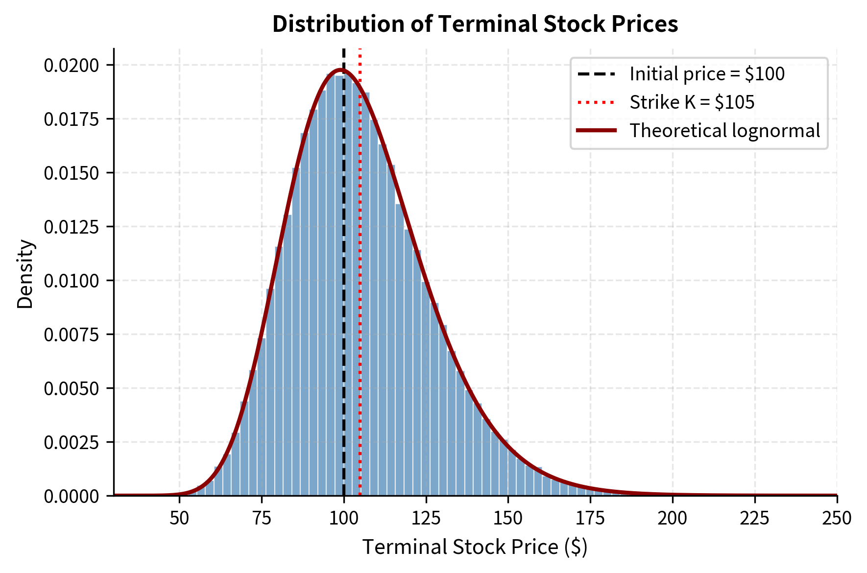
For European options that depend only on $S_T$, this single-step simulation is all we need. We simply draw a standard normal random variable, plug it into the formula, and obtain one realization of the terminal price. Repeating this process thousands or millions of times gives us the sample distribution needed for Monte Carlo estimation. However, for path-dependent options where the payoff depends on the entire trajectory of prices, we must simulate the complete path from time zero to maturity.

To generate a complete price path, we divide the time interval $[0, T]$ into $M$ discrete steps, each of size $\Delta t = T/M$. At each step, we must advance the price from its current value to the next point in time. The Euler-Maruyama discretization provides a straightforward method for this task by applying a first-order Taylor approximation to the stochastic differential equation:

where:

• $S_{t+\Delta t}$: asset price at the next time step
• $S_t$: current asset price
• $r$: risk-free interest rate
• $\sigma$: volatility
• $\Delta t$: time step size ($T/M$)
• $Z$: independent standard normal random variable

The approximation adds two terms to the current price to obtain the next price. The first term, $rS_t \Delta t$, represents the expected growth over the time step, capturing the deterministic drift component. The second term, $\sigma S_t \sqrt{\Delta t} \cdot Z$, introduces the random fluctuation, with the square root of the time step appearing because variance scales linearly with time while standard deviation scales with the square root.

However, this additive form has a subtle but important drawback: it can produce negative prices when $\Delta t$ is large or volatility is high. Since we are adding a random term that can be arbitrarily negative to a positive price, there is always some probability of ending up with a negative value, which is nonsensical for asset prices. A more stable approach uses the exact solution over each interval, applying our closed-form expression for terminal prices but treating each small interval as a mini-simulation:

where:

• $S_{t+\Delta t}$: asset price at the next time step
• $S_t$: current asset price
• $r$: risk-free interest rate
• $\sigma$: volatility
• $\Delta t$: time step size
• $Z$: independent standard normal random variable

This log-Euler scheme, sometimes called the exact discretization for GBM, preserves positivity unconditionally because the exponential function always returns positive values regardless of its input. Since the exponential of any real number is positive, and we multiply this positive quantity by the positive current price, the next price must be positive. Furthermore, this scheme is exact for geometric Brownian motion rather than just an approximation, making it the preferred method in practice for simulating GBM paths.

We build our simulations by generating standard normal random variables. As we covered in the probability fundamentals, computers produce uniform random numbers $U \sim \text{Uniform}(0, 1)$ through deterministic algorithms called pseudo-random number generators. These uniform random numbers must then be transformed to the desired distribution through mathematical operations.

The most common approaches for converting uniform random variables to standard normal random variables are:

• Box-Muller transform: This elegant method produces two independent standard normal random variables from two independent uniform random variables. Given two independent uniforms $U_1, U_2$, we compute:

  $$\begin{aligned} Z_1 &= \sqrt{-2\ln U_1}\cos(2\pi U_2) \\ Z_2 &= \sqrt{-2\ln U_1}\sin(2\pi U_2) \end{aligned}$$

  where:

  • $Z_1, Z_2$: independent standard normal random variables
  • $U_1, U_2$: independent uniform random variables on $(0, 1)$

  The transformation works by generating a random point in polar coordinates in a cleverly chosen way. The angle $2\pi U_2$ is uniformly distributed around the circle, while the squared radius $-2\ln U_1$ follows an exponential distribution (because $-\ln U$ is exponentially distributed when $U$ is uniform). Converting these polar coordinates to Cartesian coordinates using cosine and sine yields two independent standard normals. This result can be verified by computing the joint density function and showing it equals the product of two standard normal densities.

• Inverse transform: This approach exploits the fundamental theorem connecting cumulative distribution functions to uniform random variables. We apply the inverse of the standard normal CDF:

  $$Z = \Phi^{-1}(U)$$

  where:

  • $Z$: standard normal random variable
  • $\Phi^{-1}$: inverse of the standard normal cumulative distribution function
  • $U$: uniform random variable on $(0, 1)$

  The intuition here is straightforward: if $U$ represents a cumulative probability (a value between 0 and 1), then $\Phi^{-1}(U)$ tells us which value of a standard normal distribution has that cumulative probability. By mapping a uniformly distributed cumulative probability $U$ to its corresponding quantile $Z$, this method exactly reproduces the standard normal distribution. The method is conceptually elegant and directly applicable, but requires numerical approximation of $\Phi^{-1}$ since no closed-form expression exists for this function.

In practice, numerical libraries like NumPy implement highly optimized algorithms (often the Ziggurat method, which is faster than Box-Muller for modern CPU architectures) that we use directly without needing to implement these transformations ourselves.

Let's build our first Monte Carlo pricer from the ground up. We start with European calls because we can validate our results against the Black-Scholes formula. This validation is crucial: before applying Monte Carlo to exotic options where no analytical solution exists, we must verify that our implementation correctly prices options where we know the answer.

First, we compute the analytical Black-Scholes price for comparison. This serves as our ground truth against which we will measure the accuracy of our Monte Carlo estimates:

The Black-Scholes price is the benchmark for the option's theoretical value. Monte Carlo estimates should converge to this value. Agreement between these estimates and the Black-Scholes price verifies our implementation.

Now let's implement the Monte Carlo estimator. The function generates many random terminal prices, computes the payoff for each, and returns both the estimated price and a measure of statistical uncertainty:

Let's run the simulation with varying numbers of paths to observe how the estimate improves with more simulations:

The results show how Monte Carlo estimation behaves. As we increase the number of simulations by a factor of 10, the standard error decreases by approximately $\sqrt{10} \approx 3.16$. This reflects the fundamental $1/\sqrt{N}$ convergence rate that governs all Monte Carlo methods. The error in our estimate shrinks with more simulations, but it shrinks slowly. This $1/\sqrt{N}$ convergence rate is both the blessing and curse of Monte Carlo: convergence is guaranteed by the law of large numbers, but achieving high precision requires many simulations. To halve the error, you must quadruple the computational effort.

The key parameters for the Monte Carlo European option pricing model are:

• S0: Initial stock price. The starting value of the underlying asset.
• K: Strike price. The price at which you can buy (call) or sell (put) the asset.
• T: Time to maturity in years. The duration of the simulation.
• r: Risk-free interest rate. The constant rate at which the asset drifts under the risk-neutral measure.
• σ: Volatility of the underlying asset. Determines the magnitude of random price fluctuations.
• n_simulations: Number of simulated paths. Controls the precision of the estimate; higher $N$ reduces standard error.

The real power of Monte Carlo emerges when pricing path-dependent derivatives. These are options whose payoff depends not just on the terminal price $S_T$ but on the entire trajectory of the underlying asset over its lifetime. For such options, no simple closed-form solutions typically exist, and Monte Carlo becomes indispensable. We now examine three important classes of path-dependent options: Asian options, barrier options, and lookback options.

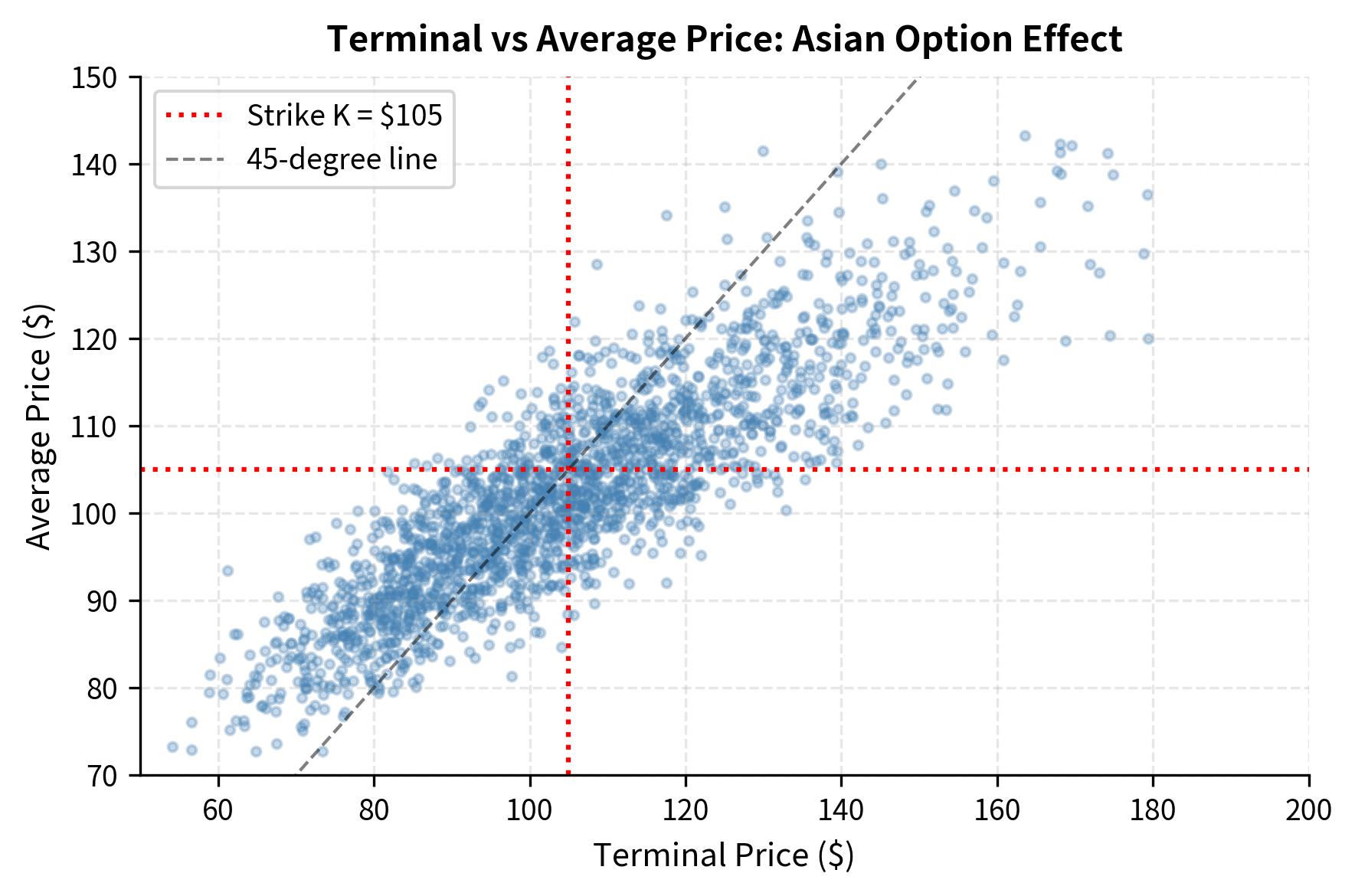
Asian options have payoffs based on the average price of the underlying over some specified period. This averaging feature makes Asian options popular in commodity markets, where buyers and sellers often care about average prices over a month or quarter rather than spot prices on a single day. An Asian call with arithmetic averaging pays the following at expiration:

where:

• $\text{Payoff}$: cash flow received at expiration
• $M$: number of averaging points
• $S_{t_i}$: asset price at observation time $t_i$
• $K$: strike price

The payoff structure compares the arithmetic average of prices observed at $M$ discrete times against the strike price. If the average exceeds the strike, you receive the difference; otherwise, the option expires worthless. This averaging creates a significant mathematical challenge: because the arithmetic average of lognormal random variables is not itself lognormal, there is no closed-form solution analogous to Black-Scholes. The distribution of the average is complex and does not yield to analytical techniques. Monte Carlo is therefore the standard approach for pricing arithmetic Asian options.

The loop-based implementation above is clear and easy to understand, showing the logic step by step. However, it is inefficient because Python loops are slow. For production use, we must vectorize the computation, replacing explicit loops with array operations that NumPy can execute efficiently:

Notice that the Asian option is cheaper than the equivalent European call. This price difference reflects a fundamental property of averaging: it reduces the effective volatility of the payoff. When you average many observations, extreme high values and extreme low values tend to cancel each other out, pulling the average toward the center of the distribution. This reduction in dispersion lowers the probability of very high payoffs, which are what make call options valuable. Asian options are therefore attractive for hedging situations where the average price is more relevant than the spot price, which is common in commodity markets where contracts reference monthly averages.

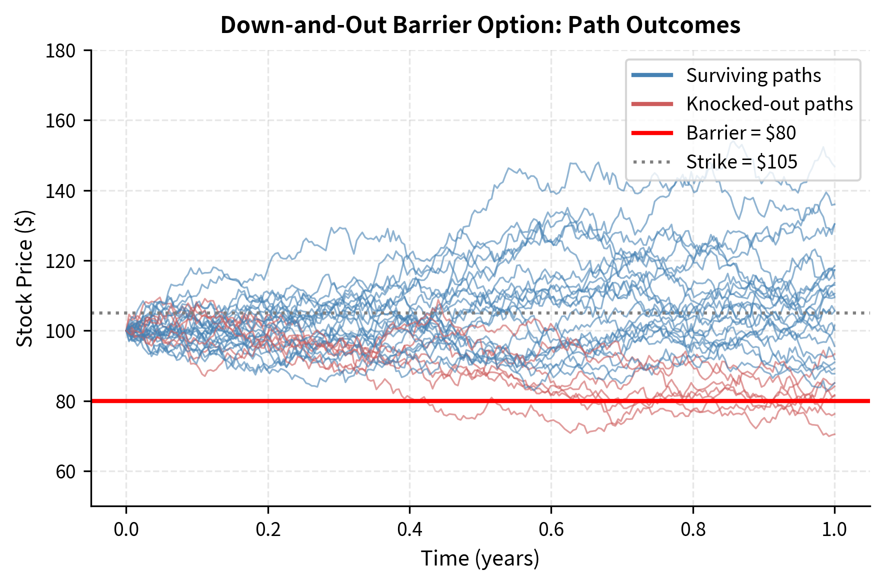
Barrier options are contracts that are activated or extinguished when the underlying crosses a specified price level called the barrier. These options are popular because they cost less than vanilla options while still providing payoff in scenarios you consider most likely. A down-and-out call, for example, pays like a regular call at expiration unless the underlying price ever falls to or below a barrier level $B$, in which case the option becomes worthless immediately and permanently:

where:

• $S_T$: asset price at time $T$
• $K$: strike price
• $B$: barrier level
• $\min_{0 \leq t \leq T} S_t$: minimum asset price realized during the option's life

The payoff condition requires monitoring whether the minimum price observed over the option's life stays strictly above the barrier. If at any point during the option's life the price touches or crosses below the barrier, the option is "knocked out" and pays nothing, regardless of where the final price ends up. This path dependency makes Monte Carlo the natural pricing approach.

The down-and-out call trades at a substantial discount to the vanilla European call because it can be knocked out. This discount compensates you for bearing knockout risk: the possibility that a temporary price decline eliminates the option even if prices subsequently recover. Barrier options are attractive when you believe the barrier will not be breached, as they offer similar upside potential at reduced cost.

Lookback options have payoffs based on the maximum or minimum price achieved during the option's life. These options give you the benefit of perfect hindsight, allowing you to exercise at the most favorable price observed. A floating-strike lookback call, for instance, pays the difference between the final price and the minimum price observed:

where:

• $\text{Payoff}$: cash flow received at expiration
• $S_T$: final asset price
• $\min_{0 \leq t \leq T} S_t$: minimum asset price realized over the life of the option

You effectively buy at the lowest price observed over the option's life and sell at the final price. This "buy low, sell at market" feature guarantees a positive payoff whenever the final price differs from the minimum, which is almost certain for any path with volatility.

Lookback options are expensive because they always pay off: as long as there is any volatility in the path, the final price will differ from the minimum. You capture the full range from minimum to maximum, receiving perfect market timing ability as a feature of the contract. These options serve as theoretical upper bounds for what options could cost if you had the ability to time the market perfectly.

The key parameters for path-dependent option simulations are:

• n_steps: Number of time steps ($M$). This determines the grid density for the path simulation. Higher $M$ reduces discretization error for continuous barriers and lookbacks.
• B: Barrier level. The price threshold that triggers the barrier condition (knock-in or knock-out).

Understanding the error in Monte Carlo estimates is essential for practical implementation. Unlike deterministic methods that give the same answer every time, Monte Carlo produces a random estimate that varies from run to run. If we repeat our simulation many times, each estimate $\hat{V}$ will differ slightly due to random sampling. This variability is not a bug but an inherent feature of the method, and it must be quantified so that you understand the precision of your estimates.

Let $X_1, X_2, \ldots, X_N$ be independent samples of the discounted payoff. Each $X_i$ represents the discounted payoff from one simulated path, and these samples are independent because we draw fresh random numbers for each path. The Monte Carlo estimator is simply the sample mean:

where:

• $\hat{V}$: Monte Carlo estimate of the option value
• $N$: number of simulations
• $X_i$: discounted payoff from the $i$-th simulation

This estimator is unbiased, meaning that its expected value equals the true option price. However, any single realization of $\hat{V}$ will deviate from the true value due to sampling variation. The central limit theorem tells us how this variation behaves: for large $N$, the sampling distribution of $\hat{V}$ is approximately normal with mean equal to the true value and variance inversely proportional to $N$:

where:

• $\hat{V}$: Monte Carlo estimate of the option value
• $V$: true option value
• $\sigma_X^2$: variance of the individual discounted payoffs
• $N$: number of simulations
• $\mathcal{N}$: normal distribution notation

Regardless of the distribution of individual payoffs (which may be highly skewed or otherwise non-normal), the average of many payoffs follows an approximately normal distribution. The approximation improves as $N$ increases, typically becoming excellent by $N = 1000$ or so.

The standard error of our estimate quantifies the typical magnitude of sampling error:

where:

• $\text{SE}(\hat{V})$: standard error of the estimator
• $\sigma_X$: standard deviation of individual discounted payoffs
• $N$: number of simulations

The standard error measures the standard deviation of the sampling distribution, telling us how much our estimate typically varies from run to run. Since we don't know the true $\sigma_X$, we estimate it from our sample using the sample standard deviation formula:

where:

• $\hat{\sigma}_X$: sample standard deviation estimator
• $N$: number of simulations
• $X_i$: discounted payoff of the $i$-th path
• $\hat{V}$: sample mean (Monte Carlo estimate)

The division by $N-1$ rather than $N$ in this formula is Bessel's correction, which makes the estimator unbiased for the true variance.

With the standard error in hand, we can construct confidence intervals that express uncertainty about the true price. A 95% confidence interval for the true price is:

where:

• $\hat{V}$: Monte Carlo estimate
• $\text{SE}(\hat{V})$: standard error of the estimator
• $1.96$: approximate $z$-score for a 95% two-sided confidence interval

This formula does not mean there is a 95% probability that the true price lies in this interval. Rather, it means that if we repeated the entire simulation many times, constructing a new confidence interval each time, 95% of those intervals would contain the true price. The distinction is subtle but important for statistical rigor.

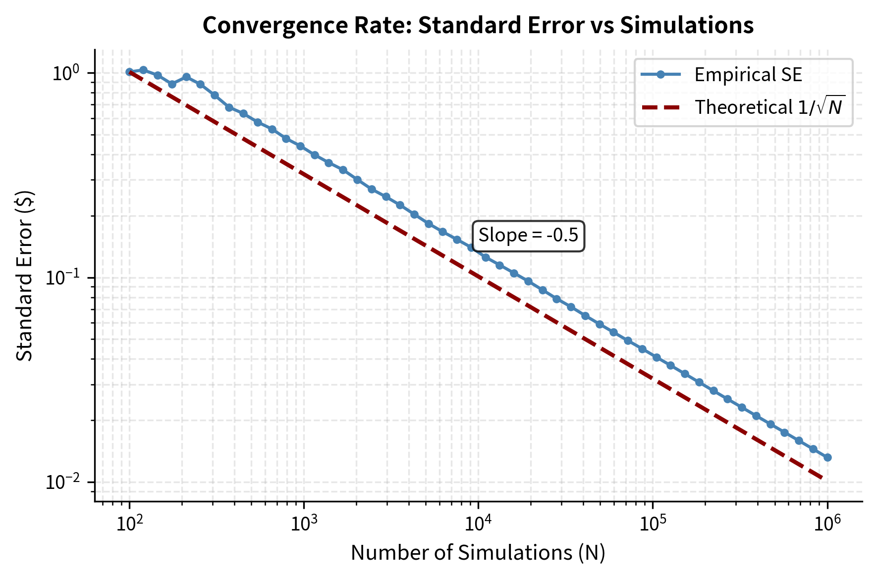
The critical insight for practical applications is that $\text{SE} \propto 1/\sqrt{N}$, meaning the standard error is inversely proportional to the square root of the number of simulations. This square-root relationship has profound implications for computational planning. To reduce the error by half, we must quadruple the number of simulations. To achieve one additional decimal place of accuracy (reducing error by a factor of 10), we need 100 times more simulations. To gain two decimal places, we need 10,000 times more paths.

This slow convergence rate motivates the search for variance reduction techniques, which we explore in the next chapter. Methods like antithetic variates, control variates, and importance sampling can dramatically reduce variance without increasing the number of paths, effectively making each simulation more informative and accelerating convergence.

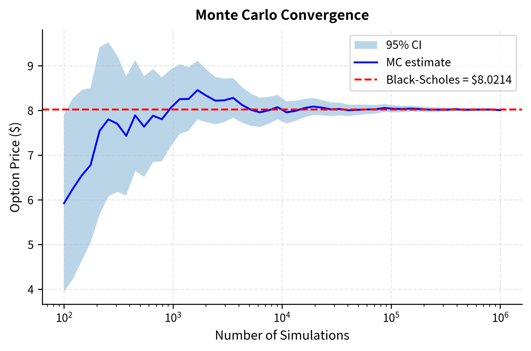
The figure illustrates convergence in action. With just 100 paths, the confidence interval spans several dollars, which is essentially useless for trading. By 10,000 paths, we achieve reasonable precision. At 1 million paths, the interval tightens to a few cents, though computational cost becomes significant.

Seeing sample paths helps build intuition for what Monte Carlo actually computes. Each path represents one possible future for the underlying asset under risk-neutral dynamics.

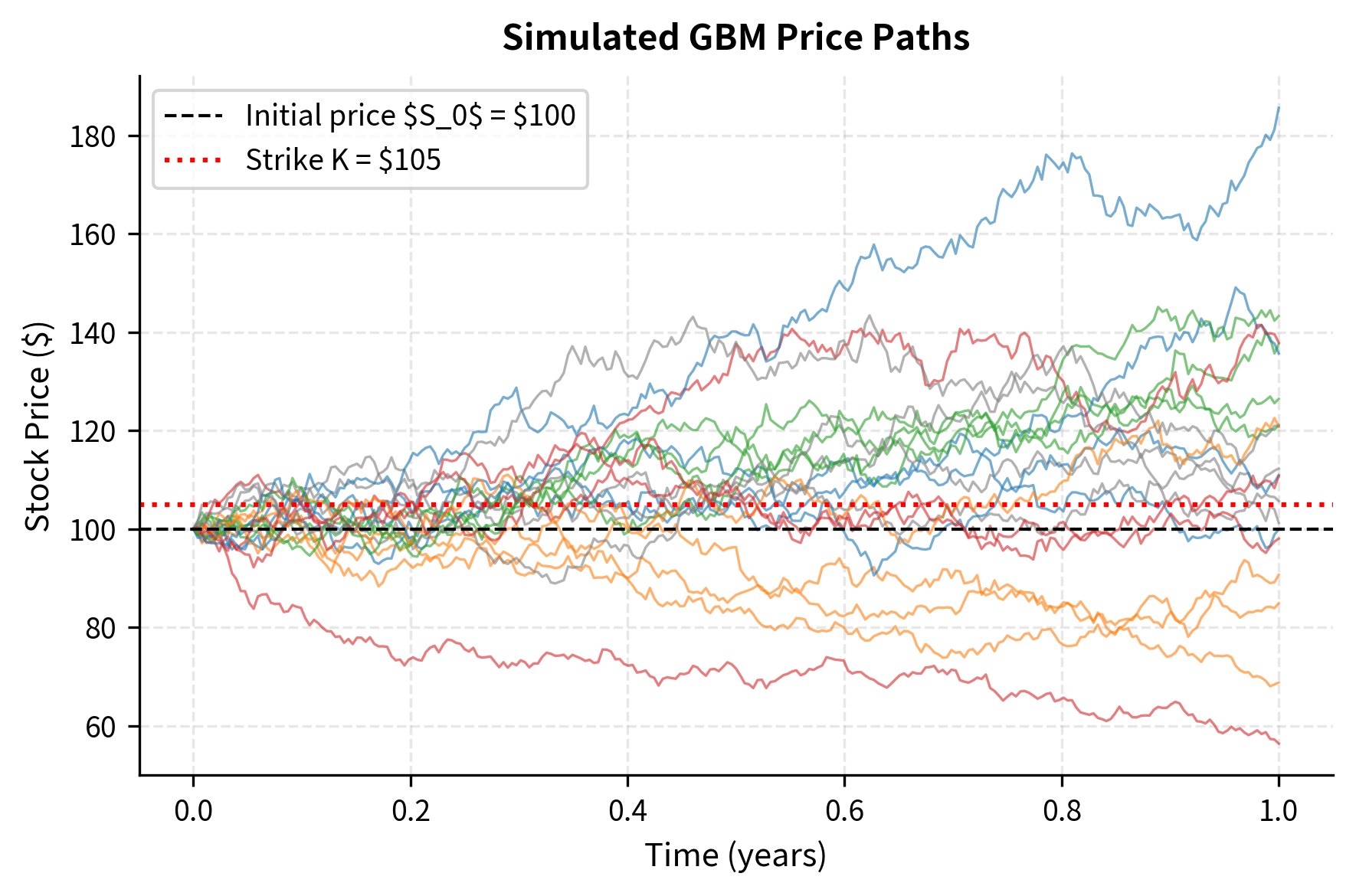
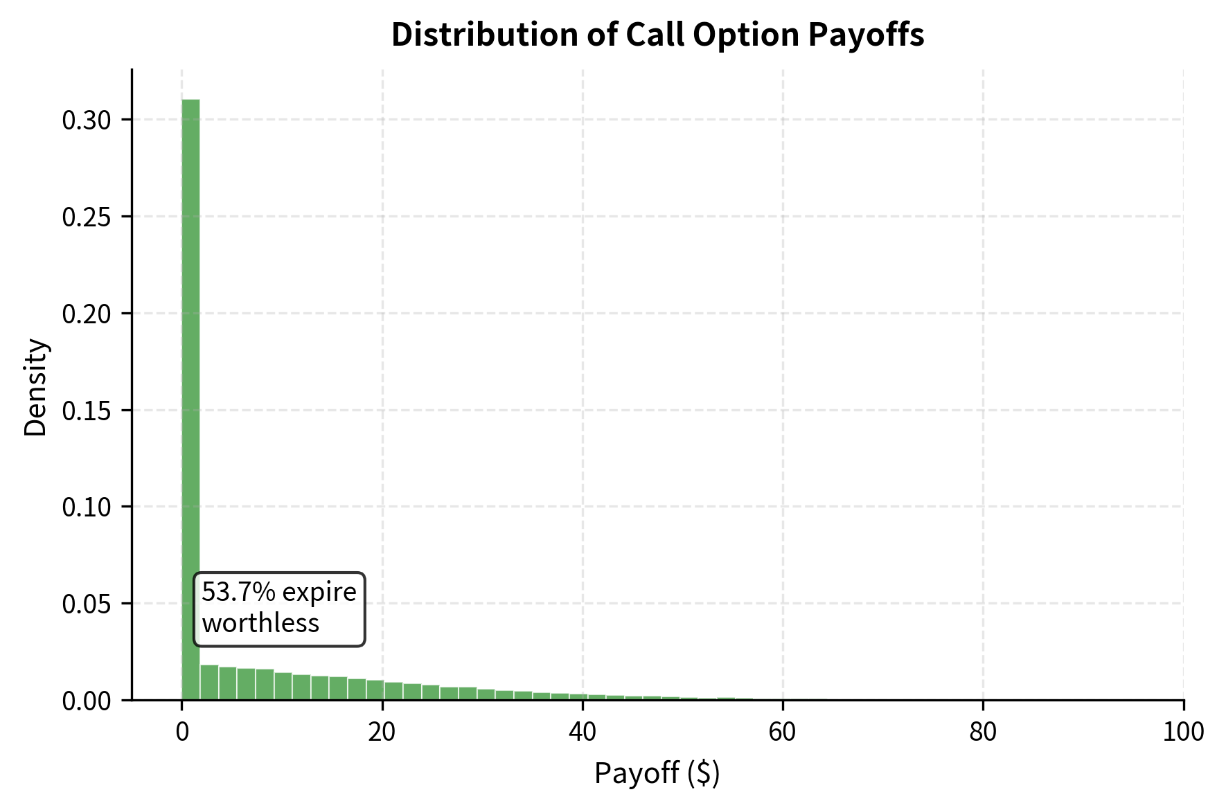
Each path tells a story. Some drift upward, finishing well above the strike and generating substantial payoffs. Others decline, finishing below the strike with zero payoff. The Monte Carlo price is the average of these discounted payoffs, which is a numerical approximation of the risk-neutral expectation.

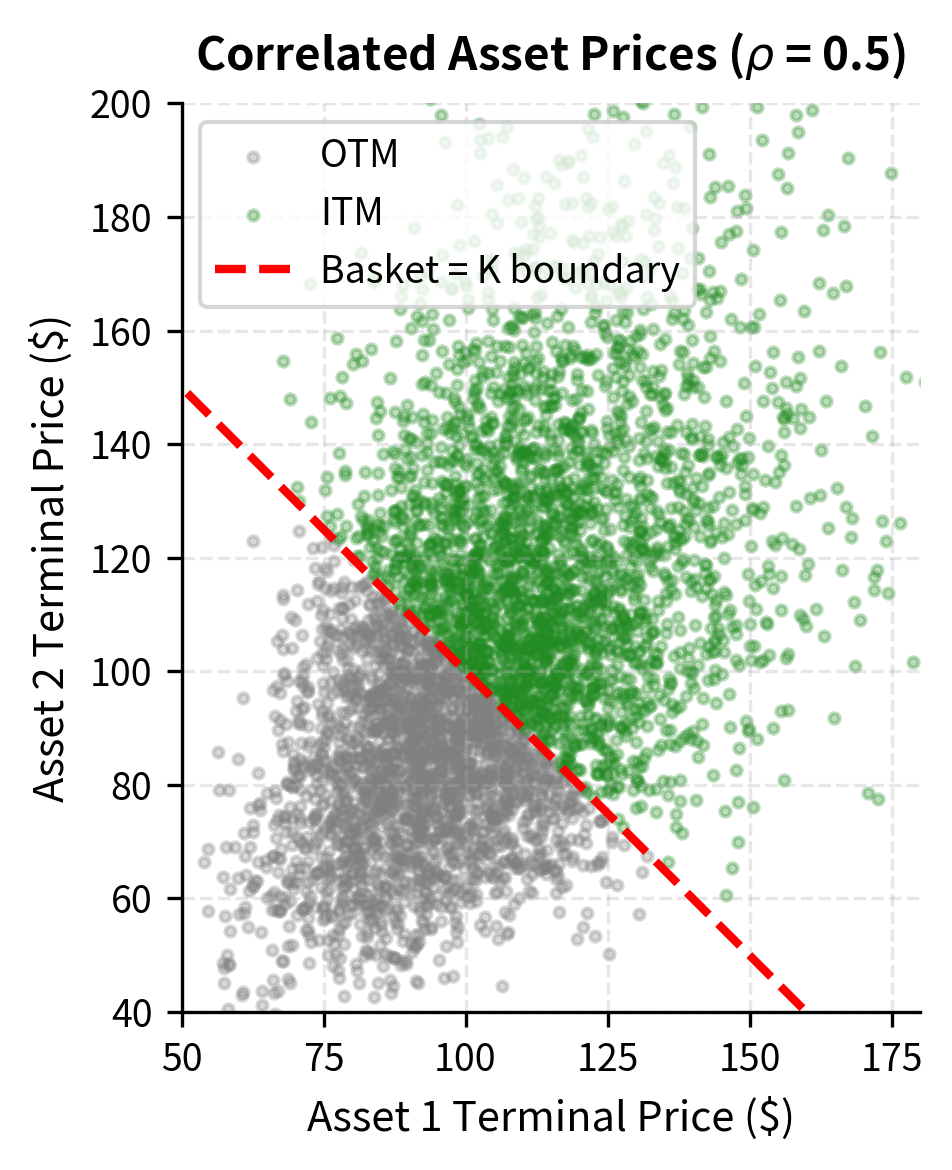
Monte Carlo extends naturally to options on multiple correlated assets, such as basket options or spread options. The key challenge in multi-asset simulation is generating random variables with the correct correlation structure. For two assets with correlation $\rho$, we generate correlated normal random variables using the Cholesky decomposition, a mathematical technique for expressing the correlation structure in a computationally convenient form.

If $Z_1, Z_2$ are independent standard normals, then the following transformation produces correlated standard normals:

where:

• $\epsilon_1, \epsilon_2$: correlated standard normal variables
• $Z_1, Z_2$: independent standard normal variables
• $\rho$: correlation coefficient
• $\rho Z_1$: component of the second asset's return driven by the common factor
• $\sqrt{1 - \rho^2} Z_2$: idiosyncratic component unique to the second asset

This construction preserves unit variance for both $\epsilon_1$ and $\epsilon_2$ (since $\rho^2 + (1-\rho^2) = 1$) while ensuring the correct correlation. The intuition is that we decompose the second asset's randomness into two parts: a portion $\rho Z_1$ that comes from the same source as the first asset (the "common factor"), and a portion $\sqrt{1 - \rho^2} Z_2$ that is unique to the second asset (the "idiosyncratic factor"). When $\rho = 1$, the second asset moves perfectly with the first. When $\rho = 0$, they are independent. When $\rho = -1$, they move in opposite directions.

For a basket call option on two assets with weights $w_1, w_2$, the payoff is simply the call payoff applied to the weighted sum:

where:

• $\text{Payoff}$: cash flow received at expiration
• $w_1, w_2$: weights of the assets in the basket
• $S_{1,T}, S_{2,T}$: asset prices at time $T$
• $K$: strike price

The basket option benefits from diversification. Even though one asset has 30% volatility, the combined basket has lower volatility due to imperfect correlation. This makes basket calls cheaper than calls on the individual assets with equivalent total notional.

For higher dimensions with more than two assets, the Cholesky decomposition of the correlation matrix generalizes this approach systematically:

where:

• $\boldsymbol{\epsilon}$: vector of correlated random variables
• $\mathbf{L}$: lower triangular Cholesky matrix
• $\mathbf{Z}$: vector of independent standard normal variables
• $\mathbf{R}$: correlation matrix ($\mathbf{R} = \mathbf{L}\mathbf{L}^T$)

The Cholesky decomposition factors the correlation matrix $\mathbf{R}$ into the product of a lower triangular matrix $\mathbf{L}$ and its transpose. By multiplying a vector of independent standard normals by $\mathbf{L}$, we obtain a vector of correlated normals with exactly the desired correlation structure. This procedure generalizes efficiently to any number of assets.

The key parameters for multi-asset basket options are:

• S: Initial asset prices ($S_{1,0}, S_{2,0}$).
• σ: Volatilities of the individual assets.
• ρ: Correlation coefficient between asset returns.
• w: Weights of the assets in the basket.

Implementing Monte Carlo in production requires attention to several practical issues beyond the basic algorithm.

The quality of pseudo-random numbers directly affects the accuracy of our estimates. Standard library generators like NumPy's default Mersenne Twister are adequate for most applications. For very high-precision work, low-discrepancy sequences (quasi-Monte Carlo) provide more uniform coverage of the probability space, improving convergence, though they sacrifice true randomness.

Vectorized operations in NumPy run orders of magnitude faster than Python loops. Always generate all random numbers at once and use array operations:

For production systems, GPU acceleration with libraries like CuPy or JAX can further speed up simulations by orders of magnitude.

For reproducibility in research and debugging, always set and document random seeds. For production risk systems, use different seeds for independent runs and aggregate results to ensure robustness across random number sequences.

Storing all paths in memory becomes prohibitive for millions of paths with hundreds of steps. When only the payoff matters, compute it incrementally:

Monte Carlo simulation changed derivative pricing by enabling us to price instruments that lack analytical solutions. Before Monte Carlo became practical (enabled by increasingly powerful computers in the 1980s and 1990s), path-dependent exotics were priced by crude approximations or not at all. Today, Monte Carlo underlies the pricing of exotic equity derivatives, complex structured products, CVA and XVA calculations, and virtually any derivative where simpler methods fail.

Yet Monte Carlo has significant limitations. The $1/\sqrt{N}$ convergence rate means that each additional digit of precision requires 100 times more computation. For options requiring real-time pricing, like vanilla puts and calls on a trading desk, Monte Carlo is too slow. Black-Scholes formulas compute instantly, while Monte Carlo with acceptable precision might take seconds or minutes. The next chapter on variance reduction techniques addresses this by extracting more information from each simulation, effectively accelerating convergence without more paths.

Monte Carlo also struggles with early exercise. American options can be exercised at any time, and determining the optimal exercise boundary requires knowing the continuation value at each point. The standard backward-induction approach of binomial trees doesn't apply directly. Advanced techniques like Longstaff-Schwartz regression-based Monte Carlo address this, but add complexity and computational cost.

Another limitation is sensitivity calculation. The Greeks (essential for hedging) require derivatives of the option price with respect to parameters. Naive finite-difference approaches (bump-and-reprice) introduce additional noise and computational burden. Pathwise derivatives and likelihood ratio methods provide alternatives, but each has its own complications.

Despite these challenges, Monte Carlo remains indispensable. When you encounter a derivative with path dependencies, multiple assets, complex barriers, or other exotic features, Monte Carlo is typically the first tool you reach for. Its flexibility, specifically the ability to price nearly anything that can be simulated, makes it a cornerstone of quantitative finance.

This chapter developed Monte Carlo simulation as a powerful numerical method for derivative pricing. The core principle is simple: simulate many possible futures under risk-neutral dynamics, compute payoffs, and average.

We saw that for European options depending only on terminal prices, a single simulation step using the exact GBM solution suffices. For path-dependent options like Asians, barriers, and lookbacks, we simulate full trajectories using the log-Euler discretization scheme.

The Monte Carlo estimator converges to the true price as the number of simulations grows, with standard error proportional to $1/\sqrt{N}$. Confidence intervals quantify uncertainty in our estimates. This slow convergence motivates variance reduction techniques covered in the next chapter.

Practical implementation requires vectorized code for efficiency, proper random number generation, and sometimes batched processing for memory management. Multi-asset options extend naturally through correlated random variables generated via Cholesky decomposition.

Monte Carlo's great strength is flexibility: it handles virtually any payoff structure. Its weakness is speed: when closed-form solutions exist, they are vastly faster. You must know when each tool applies and match method to problem.

Ready to test your understanding? Take this quick quiz to reinforce what you've learned about Monte Carlo simulation for derivative pricing.