

Learn to compute implied volatility using Newton-Raphson and bisection methods. Explore volatility smile, skew patterns, and the VIX index with Python code.
Choose your expertise level to adjust how many terms are explained. Beginners see more tooltips, experts see fewer to maintain reading flow. Hover over underlined terms for instant definitions.
Implied Volatility and Volatility Smile
In the Black-Scholes-Merton framework we developed in Chapter 6, volatility enters as a fixed parameter representing the constant diffusion of the underlying asset's returns. We treated this parameter as an input, something we might estimate from historical returns. Practitioners discovered something profound. Instead of estimating volatility and using it to calculate a price, you can reverse the process. Given an observed market price, you can solve for the volatility that produces a Black-Scholes theoretical price matching that market price. This backed-out volatility is called implied volatility.
Implied volatility transformed how traders think about options. Instead of quoting options in dollar terms, market participants began quoting them in volatility terms. When a trader says "the 100-strike call is trading at 25 vol," everyone understands exactly how expensive that option is relative to its theoretical value. More importantly, practitioners discovered systematic patterns when computing implied volatilities across different strikes and maturities. These patterns directly contradicted the Black-Scholes assumption of constant volatility. These patterns are the volatility smile and volatility skew, which reveal the market's collective assessment of tail risks, jump probabilities, and the inadequacy of the lognormal assumption for asset returns.
This chapter develops the concept of implied volatility from first principles, shows you how to compute it numerically, and explores the rich structure of the volatility surface. Understanding these patterns is essential for anyone who trades options, manages option portfolios, or builds derivative pricing models.
Defining Implied Volatility
Recall from Chapter 6 that the Black-Scholes formula for a European call option is:
This elegant formula expresses the theoretical value of a European call option as the difference between two probability-weighted terms. The first term, , represents the expected present value of receiving the stock upon exercise, accounting for the probability that the option finishes in the money under the risk-neutral measure and weighted by the stock price's drift. The second term, , represents the present value of the payment you would make if you exercise the option, weighted by the risk-neutral probability that you actually do exercise. The notation and components deserve careful attention.
- : current spot price of the underlying asset
- : strike price of the option
- : time to expiration in years
- : risk-free interest rate
- : volatility of the underlying asset returns
- : cumulative standard normal distribution function
- : standardized moneyness adjusted for volatility and time
- : adjusted for the volatility over the option's life
- : the expected value of the asset at expiration, conditional on the option being in-the-money
- : the present value of the strike price, weighted by the probability of exercise
The parameter captures how far the current stock price is from the strike in standardized units. It adjusts for the expected drift and the accumulation of uncertainty over the option's life. The numerator contains the log-moneyness (measuring how far the current price stands from the strike in percentage terms) plus an adjustment that accounts for the expected appreciation under the risk-neutral measure. The denominator normalizes this measure by the total expected standard deviation of returns over the option's life, converting everything into units of standard deviations.
The inputs , , , and are all observable market variables. The current stock price is available on any trading screen, the strike price is specified in the option contract, the time to expiration follows from the contract's expiration date, and the risk-free rate can be approximated from Treasury bill yields or other money market instruments. Volatility is the only unobservable parameter. It describes how much the underlying asset's returns fluctuate, but this quantity cannot be directly observed because it pertains to the future. Given a market price , the implied volatility is the value of that satisfies:
This equation establishes a relationship between the theoretical Black-Scholes world and the actual market. The left side represents the theoretical price that emerges from the model when we use a particular volatility assumption. The right side represents the price at which actual buyers and sellers agree to trade. When these two quantities match, we have found the volatility that the market is implicitly using to price the option. The components of this equation deserve explicit identification:
- : theoretical Black-Scholes option price
- : implied volatility parameter to be solved for
- : observed market price of the option
- : observable market inputs (spot, strike, time, rate)
Implied volatility is the volatility parameter that, when substituted into the Black-Scholes formula, produces a theoretical price equal to the observed market price of an option. It represents the market's consensus expectation of future volatility over the option's remaining life.
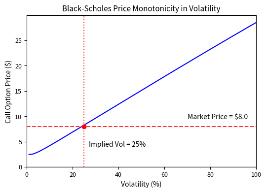
The concept of implied volatility rests on a crucial mathematical property: the Black-Scholes price is strictly increasing in volatility. When volatility is zero, the call option price equals its discounted intrinsic value (or zero if out of the money). As volatility increases without bound, the call option price approaches the current stock price. Because the price increases monotonically and continuously between these bounds, for any market price within this range, there exists exactly one volatility value that produces that price. This uniqueness guarantees that implied volatility is well-defined.
For put options, we can either solve the analogous equation using the Black-Scholes put formula, or use put-call parity (which we derived in Chapter 9 on option basics) to convert put prices to equivalent call prices first. By put-call parity, a call and put with the same strike and expiry should have the same implied volatility. This equivalence arises because put-call parity is a model-free relationship based only on no-arbitrage arguments, so any systematic difference in implied volatility between a call and put at the same strike would create an arbitrage opportunity.
Why Implied Volatility Matters
Implied volatility serves several key functions in practice:
As a quoting convention: Traders quote options in volatility terms because it provides a standardized measure that allows comparison across strikes, maturities, and even different underlying assets. A 25% implied vol on an SPX option means something similar to 25% implied vol on an individual stock option. Even though the dollar prices differ enormously, the standardized volatility measure makes them comparable.
As a market expectation: Implied volatility reflects the market's forward-looking assessment of uncertainty. If implied volatility is high, the market expects large price movements. If it's low, the market expects calm. Unlike historical volatility, which looks backward at what already happened, implied volatility looks forward.
As a trading signal: When implied volatility differs significantly from a trader's own volatility forecast, opportunities arise. Buying options when implied vol is "too low" and selling when it's "too high" is the foundation of volatility trading strategies.
As a risk indicator: Implied volatility spikes during market stress. The most famous measure, the VIX index, aggregates implied volatilities from S&P 500 options into a single "fear gauge" that captures market anxiety.
Computing Implied Volatility
The equation cannot be solved analytically for . The Black-Scholes formula combines the cumulative normal distribution function, logarithms, and exponentials in ways that prevent algebraic isolation of . Therefore, we must use numerical methods. This is a root-finding problem: we seek the root of:
The function measures the discrepancy between the theoretical price at volatility and the target market price. When this discrepancy equals zero, we have found our implied volatility. The structure of this problem is particularly favorable for numerical methods because is smooth, continuous, and monotonically increasing in . These properties ensure that root-finding algorithms will converge reliably. The components of the objective function are:
- : objective function to minimize (find zero)
- : volatility parameter
- : Black-Scholes pricing function
- : target market price
Several root-finding algorithms can solve this problem. The two most common are the Newton-Raphson method and the bisection method.
The Newton-Raphson Method
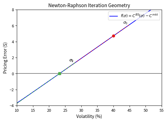
Newton-Raphson is an iterative algorithm that uses both the function value and its derivative to make intelligent updates. The intuition is geometric. At each iteration, we approximate the function by its tangent line at the current point and move to where that tangent line crosses zero. When the function is reasonably well-behaved, this linear approximation improves with each iteration, leading to rapid convergence. The update formula is:
The formula evaluates the error to measure the distance from zero and divides by the derivative to compute the adjustment needed. The ratio has a natural interpretation: it measures how far we need to travel along the tangent line to reach zero. The negative sign ensures we move in the direction that reduces the function value when it's positive. Each component plays a specific role:
- : updated volatility estimate
- : current volatility estimate
- : error between theoretical and market price at current estimate
- : derivative of the error function with respect to volatility
For our problem, , so . Since the market price is a constant (we observe it from the market), its derivative is zero, and the derivative of our objective function equals the derivative of the Black-Scholes price with respect to volatility. This derivative is precisely vega, which we studied in Chapter 7 on the Greeks:
Vega measures how sensitive the option price is to small changes in volatility. The formula reveals that vega is always positive (both , , and the probability density are positive), confirming that option prices increase with volatility. The magnitude of vega depends on the spot price , the square root of time , and the probability density at . Options that are at-the-money (where is close to zero and is maximized) have the largest vega. The components of this formula are:
- : vega, the sensitivity of option price to volatility
- : spot price
- : time to expiration
- : standardized moneyness parameter
- : standard normal probability density function evaluated at
The probability density is the bell-curve function evaluated at . It peaks when and decays exponentially as moves away from zero in either direction. This explains why at-the-money options have the highest vega: they are precisely the options where is closest to zero.
Substituting vega into the Newton-Raphson update formula, we obtain:
The numerator is the pricing error: how much the Black-Scholes price at our current volatility estimate exceeds (or falls short of) the market price. The denominator is vega, which tells us how much the price changes per unit change in volatility. The ratio gives us the volatility adjustment needed to eliminate the pricing error under a linear approximation. Each term serves a distinct purpose:
- : new volatility estimate
- : current volatility estimate
- : Black-Scholes price calculated using
- : observed market price
- : vega calculated using
Newton-Raphson converges quickly (quadratically) when it works, but it can fail to converge if the initial guess is poor or if vega becomes very small (deep in-the-money or out-of-the-money options with short expiries). Quadratic convergence means the number of correct digits roughly doubles with each iteration. For example, if you have 2 correct digits after one iteration, you will have approximately 4 after the next, then 8, then 16. This rapid convergence makes Newton-Raphson extremely efficient when it succeeds.
The Bisection Method
Bisection is more robust but slower. It requires bracketing the solution between two values and such that and have opposite signs. The intermediate value theorem guarantees that a continuous function that changes sign must cross zero somewhere in the interval. Since the Black-Scholes price is monotonically increasing in (vega is always positive for vanilla options), we can always bracket the solution between (giving the intrinsic value) and some large (giving a price approaching for calls).
The bisection method repeatedly halves the interval, selecting the half that still brackets the root. At each step, we compute the midpoint and evaluate . If this value has the same sign as , the root lies in the upper half, so we update . Otherwise, the root lies in the lower half, and we update . Either way, we have halved the interval containing the root.
Bisection converges linearly, adding roughly one bit of precision per iteration. This means that to achieve machine precision (about 16 decimal digits), we need roughly 53 iterations. While slower than Newton-Raphson, bisection is guaranteed to converge as long as we start with a valid bracket, making it an excellent fallback method for difficult cases.
Implementation
Let's implement both methods and compare their performance.
The Newton-Raphson implementation uses vega directly:
The bisection method provides a robust fallback:
Let's test both methods on a sample option:
The Newton-Raphson and bisection methods both converge to the same implied volatility. When we reprice the option using this implied volatility, we get a price that matches the market price to within numerical precision. This demonstrates that the root-finding problem is well-posed. Given a valid market price within the no-arbitrage bounds, a unique implied volatility exists that exactly reproduces that price. The Newton-Raphson method typically converges in 3-5 iterations, while bisection requires more iterations but guarantees convergence.
Comparing Convergence Speed
Newton-Raphson typically converges in 3-5 iterations, while bisection requires roughly 50 iterations for similar precision. Let's visualize the convergence:
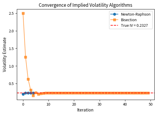
Newton-Raphson reaches the true value in about 4 iterations, while bisection is still oscillating around the true value after 50 iterations. For practical applications involving thousands of option prices, the speed difference matters significantly.
Key Parameters
Key parameters for implied volatility computation and convergence analysis include:
- : Spot price of the underlying asset, used in all Black-Scholes calculations. Observable from market quotes.
- : Strike price of the option. Determines moneyness and convergence properties. Deep options present numerical challenges because vega is small.
- : Time to expiration in years. Short-dated options are numerically challenging because vega becomes very small near expiration.
- : Risk-free interest rate affecting present value calculations. Use rates matching the option's maturity, typically from Treasury yields or SOFR.
market_price: Observed option price, the target value to match. Must lie within no-arbitrage bounds.initial_guess: Starting volatility estimate for Newton-Raphson, typically 0.2. Good starting points accelerate convergence.tolerance: Convergence criterion, typically 1e-8. Smaller values require more iterations but yield more accurate results.max_iterations: Maximum iterations before failing, typically 100. Prevents infinite loops.sigma_lowandsigma_high: Bracketing bounds for bisection method. Must contain the true solution. The lower bound should be small and positive, and the upper bound should be large enough for any realistic volatility.
The Volatility Smile
If the Black-Scholes model were correct, the log-returns of the underlying asset would be normally distributed with constant volatility . In this ideal world, every option on the same underlying with the same expiration date would have the same implied volatility, regardless of strike price. You could compute the implied volatility from any option, and it would equal the "true" volatility .
Reality contradicts this prediction. When practitioners compute implied volatilities across different strikes for options with the same expiration, they find systematic patterns. These patterns are not random noise but persistent features that appear across markets and time periods, indicating fundamental inadequacies in the Black-Scholes assumptions.
The Classic Smile Pattern
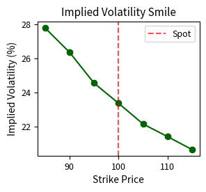
In many markets, particularly foreign exchange, implied volatility is lowest for at-the-money options and increases as you move to either in-the-money or out-of-the-money strikes. When plotted against strike price, this pattern resembles a smile: hence the name. The smile indicates that options with strikes far from the current spot price trade at higher implied volatilities than at-the-money options. This pattern seemingly contradicts the notion that there is a single "true" volatility for the underlying asset.
The smile pattern reveals that market participants collectively believe extreme price movements are more likely than the lognormal distribution would suggest. By pricing out-of-the-money options at higher implied volatilities, the market effectively assigns more probability mass to the tails of the return distribution than the Black-Scholes model assumes.
Let's simulate what market prices might look like if they embedded a volatility smile and then recover the implied volatilities:
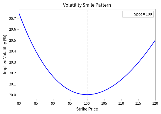
The symmetric smile pattern shows that out-of-the-money calls (high strikes) and out-of-the-money puts (low strikes) trade at higher implied volatilities than at-the-money options. This means the market assigns higher probability to large moves in either direction than the lognormal distribution would predict. The quadratic shape of the smile reflects the increasing premium demanded for options that require increasingly extreme price movements to finish in the money.
The Volatility Skew
In equity markets, especially after the stock market crash of October 1987, a different pattern emerged: the volatility skew. Rather than being symmetric, implied volatility is highest for low strikes (out-of-the-money puts) and decreases as strikes increase. This asymmetric pattern reflects the market's fear of downside crashes. The skew represents the cost of crash insurance. Investors are willing to pay significant premiums to protect against sudden, severe market declines.
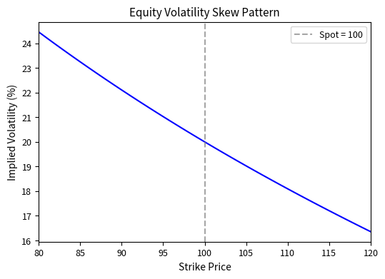
The skew pattern is sometimes called the "smirk" because of its asymmetric shape. It emerged dramatically after Black Monday in 1987, when the S&P 500 fell over 20% in a single day. Before that crash, equity option implied volatilities were relatively flat across strikes. The crash demonstrated that tail events were far more likely than lognormal models predicted, and the skew has persisted ever since as a permanent feature of equity option markets.
Why Do Smiles and Skews Exist?
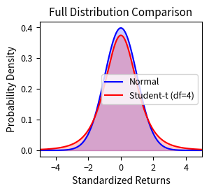
The volatility smile reveals gaps in the Black-Scholes model's assumptions about market dynamics. The model assumes log-returns follow a normal distribution, but as we discussed in Part III, Chapter 1 on stylized facts of financial returns, actual returns exhibit fat tails (leptokurtosis), skewness, and volatility clustering. These deviations from normality explain the smile and skew patterns.
Fat Tails and Leptokurtosis
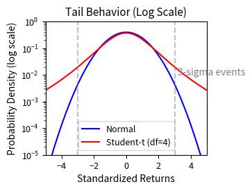
Real return distributions have fatter tails than the normal distribution. This phenomenon, known as leptokurtosis, means that extreme moves occur more frequently than Gaussian models predict. The normal distribution assumes returns decay exponentially in the tails. Empirical evidence shows financial returns decay more slowly, following a power law in many cases.
To price this tail risk correctly, the market demands higher premiums for out-of-the-money options. These options only pay off when extreme moves occur. Since such moves happen more frequently than the Black-Scholes model assumes, this translates to higher implied volatilities for strikes far from the current price. The smile pattern emerges naturally as the market's acknowledgment of fat tails within the Black-Scholes framework.
Consider a 3-standard-deviation move. Under a normal distribution, this should occur about 0.3% of the time (roughly once every 300 days). In reality, such moves happen several times per year in equity markets. Traders learned this lesson painfully: selling cheap out-of-the-money options that expired in-the-money during crashes led to massive losses. The survivors now price tail-risk options with appropriate premiums.
Negative Skewness in Returns
Equity returns are negatively skewed. Large down moves are more common than large up moves. This asymmetry in the return distribution justifies the equity skew pattern: out-of-the-money puts (which pay off in crashes) should be more expensive than out-of-the-money calls (which pay off in rallies), implying higher volatility for lower strikes.
The asymmetry arises from leverage effects and market dynamics. When stock prices fall, companies become more leveraged (debt-to-equity ratios rise), which increases their risk and volatility. Additionally, market panics create selling cascades and liquidity evaporation that amplify downward moves. These mechanisms are largely absent for upward moves. Markets tend to climb gradually but fall quickly, leading to the familiar pattern of slow, steady bull markets that are punctuated by sharp, sudden corrections.
Stochastic Volatility
The Black-Scholes model assumes volatility is constant, but we observe volatility changing over time and correlating with the underlying asset's price. When volatility is uncertain, option prices should reflect this additional risk. Models that incorporate stochastic volatility, which we'll explore in Chapter 18 on modeling volatility, naturally produce smile patterns even when the underlying asset follows a more general process.
The intuition is straightforward: if volatility can change, then an out-of-the-money option has two ways to end up in the money. Either the underlying can move directly there, or volatility can increase first (making larger moves more likely) and then the underlying can move. This second pathway adds value to out-of-the-money options, beyond what constant-volatility models predict. The possibility that volatility might spike before expiration creates additional value for options that would benefit from such an increase, and this additional value manifests as higher implied volatility.
Jump Risk
Asset prices occasionally jump discontinuously. Earnings announcements, mergers, regulatory decisions, and market crashes can cause instant price changes that dwarf typical daily moves. These jumps represent information arriving suddenly rather than gradually, and they cannot be captured by continuous Brownian motion.
The Black-Scholes model with continuous Brownian motion cannot capture this behavior. Jump-diffusion models, where prices follow Brownian motion punctuated by occasional random jumps, generate smile patterns because the jumps add probability mass to the tails of the return distribution. The market prices options as if jumps might occur, even when such events are rare, and this additional risk premium appears as elevated implied volatility for out-of-the-money options.
Supply and Demand for Protection
Beyond pure modeling arguments, market structure matters. Institutional investors systematically buy downside protection (puts) to hedge their equity portfolios. This persistent demand raises put prices and implied volatilities for low strikes. Pension funds, insurance companies, and other fiduciaries have regulatory or policy mandates to protect against large losses, creating a structural bid for puts.
Conversely, many investors sell covered calls against their stock holdings, increasing supply and suppressing implied volatilities for high strikes. Retail investors and yield-seeking funds systematically write calls to generate income, adding to the supply of upside options. These supply-demand imbalances persist over time because they reflect the fundamental needs of different market participants, not temporary trading opportunities.
The Volatility Surface
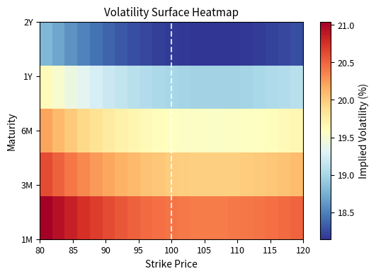
We have examined implied volatility across strikes for a single expiration. In reality, options trade across many expiration dates, and the implied volatility structure varies with both strike and maturity. This two-dimensional structure is called the volatility surface.
The volatility surface is the three-dimensional plot of implied volatility as a function of strike price and time to expiration. It captures the complete structure of option prices across all strikes and maturities for a given underlying asset.
The volatility surface encapsulates all the information embedded in option prices across the entire market. Rather than analyzing individual options, traders and risk managers view the entire surface as a single object. It shifts and deforms in response to market events. Understanding the shape and dynamics of this surface is crucial for pricing exotic options, managing portfolio risk, and identifying relative value opportunities.
Let's construct and visualize a volatility surface:
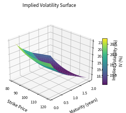
The surface exhibits several characteristic features:
Skew along the strike dimension: For any fixed maturity, implied volatility decreases as strike increases (the equity skew pattern). This reflects the market's assessment that downside risk exceeds upside risk, with out-of-the-money puts commanding a premium over out-of-the-money calls.
Term structure along the maturity dimension: Implied volatility often varies with time to expiration. When near-term uncertainty is high, such as before an earnings announcement or election, short-dated options have higher implied vol than long-dated options. In calmer periods, the term structure may invert. The term structure captures how the market's uncertainty evolves over different time horizons.
Smile attenuation with maturity: The smile or skew tends to flatten for longer maturities. A 3-month option might show a steep skew, while a 2-year option shows a milder slope. This occurs because over longer horizons, the distribution of returns becomes more stable and less influenced by near-term tail risks. The central limit theorem suggests that as the time horizon increases, the sum of many small returns approaches a normal distribution, which would imply a flatter smile.
Visualizing Smile Across Maturities
A useful way to examine the surface is to plot implied volatility versus strike for several maturities simultaneously:
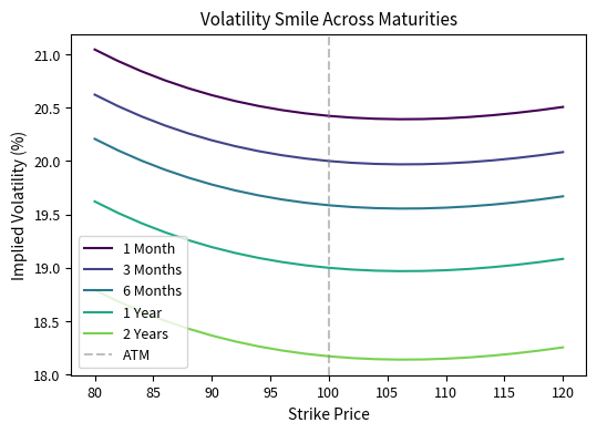
Notice how the 1-month curve has the steepest skew, while the 2-year curve is nearly flat. This pattern reflects the mean-reversion of volatility: over short horizons, current market conditions dominate, but over longer horizons, volatility tends to revert toward historical averages. The market recognizes that extreme conditions are unlikely to persist indefinitely, so long-dated options do not command the same tail-risk premium as short-dated options.
Practical Applications
The VIX Index: Measuring Market Fear
The CBOE Volatility Index (VIX) is perhaps the most famous application of implied volatility. It represents the market's expectation of 30-day volatility for the S&P 500 index, derived from the prices of SPX options across a range of strikes and two near-term expirations. The VIX has become a standard benchmark for market stress and is widely used by traders, portfolio managers, and the financial media as a barometer of investor sentiment.
The VIX calculation uses a model-free approach that does not rely on Black-Scholes assumptions. Instead of computing implied volatility from a single option, the VIX methodology integrates option prices across out-of-the-money calls and puts to extract the market's implied variance. This approach captures the entire distribution of expected returns implied by option prices across all strikes, not just at-the-money. The formula is:
This formula encapsulates the market's expectation of variance over the next 30 days. The first term sums up the contributions from all out-of-the-money options, where each option's contribution is weighted by the width of the strike interval divided by the square of the strike price. The exponential factor converts prices to forward prices, and is the observed market price. The second term is a small adjustment that accounts for the gap between the forward price and the nearest strike.
Each component of this formula has a specific interpretation:
- : VIX variance (squared volatility)
- : time to expiration
- : risk-free interest rate
- : strike price of the -th out-of-the-money option
- : interval between strike prices
- : midpoint of the bid-ask spread for the option with strike
- : forward index level derived from option prices
- : first strike price below the forward index level
The formula decomposes variance into two parts: the summation term captures the weighted prices of out-of-the-money options across all strikes, while the second term adjusts for the difference between the forward price and the central strike . This decomposition allows the VIX to reflect the entire shape of the implied volatility surface, not just a single point.
The VIX is quoted in annualized volatility points. A VIX of 20 means the market expects the S&P 500 to move approximately over the next 30 days. This reflects the square root of time scaling that converts annual volatility to monthly terms. Variance accumulates linearly with time while volatility scales with the square root of time.
This interpretation guide shows how market participants read VIX levels. Values below 15 indicate complacency, where investors expect minimal volatility and see little need for downside protection. Normal conditions (15-20) represent typical market behavior with moderate uncertainty. When VIX rises above 20, it signals increasing concern about future moves. Values above 35 indicate genuine crisis conditions where large daily swings are expected.
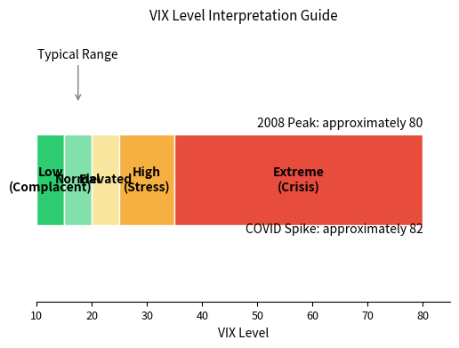
The VIX spiked to 80 during the 2008 financial crisis and exceeded 80 again briefly in March 2020 during the COVID-19 market crash. These extreme readings indicated that the market expected daily moves of approximately , which is extraordinary for a broad market index.
Volatility as a Trading Unit
Professional options traders quote prices in volatility terms rather than dollar terms. This convention simplifies communication and comparison.
When a trader says "I'll bid 22 vol for the 90 put," they mean they are willing to buy the 90-strike put at an implied volatility of 22%. Similarly, "The 100-105 call spread is offered at 1 vol" means the spread can be bought at a net implied volatility of 1%.
This quoting convention also facilitates relative value analysis. A trader might observe that the 95-strike put trades at 25 vol while the 105-strike call trades at only 18 vol. The 7-vol difference reflects the equity skew. If the trader believes the skew is too steep, they might sell the 95 put and buy the 105 call to capture the difference.
Risk Management with the Volatility Surface
For portfolios of options, risk managers need to understand how the portfolio's value changes when the entire volatility surface shifts. The key risks include parallel shift risk (the entire surface moves up or down uniformly, similar to vega risk aggregated across the portfolio), skew risk (the slope changes: if skew steepens, low-strike options become relatively more expensive), and term structure risk (the relationship between short-dated and long-dated implied vol changes, affecting portfolios with mixed maturities).
Sophisticated traders hedge not just the level of implied volatility but also its slope and curvature across strikes and maturities.
Worked Example: Building an Implied Volatility Smile from Market Data
Let's extract implied volatilities from hypothetical market prices and analyze the resulting smile.
The table reveals a clear volatility skew pattern characteristic of equity options. Low strikes (out-of-the-money puts converted to call parity) show higher implied volatilities than high strikes (out-of-the-money calls), reflecting the market's assessment that downside moves are more likely and more severe than upside moves of similar magnitude. The at-the-money strike shows intermediate volatility levels.
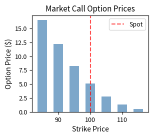
The analysis reveals a typical equity skew. A trader observing this pattern might consider selling the expensive low-strike options and buying the cheap high-strike options if they believed the skew was too extreme.
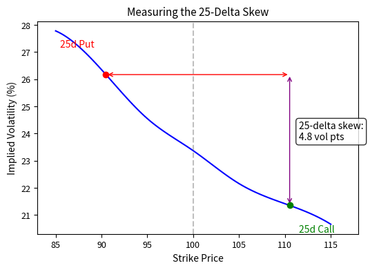
Measuring the Skew
A common metric for quantifying the skew is the difference between the implied volatility at the 25-delta put and the 25-delta call. Delta measures how far in or out of the money an option is in probability terms. Roughly speaking, a 25-delta put corresponds to a strike about 1 standard deviation below spot, and a 25-delta call corresponds to a strike about 1 standard deviation above. By using delta rather than fixed strike prices, the skew metric adjusts automatically for different volatility levels and times to expiration, making it comparable across different market conditions.
We can estimate the skew from our data by interpolating:
The 25-delta skew measures the difference in implied volatility between options that are roughly one standard deviation away from the current price. The put at a lower strike implies higher volatility, while the call at a higher strike implies lower volatility. The difference quantifies the steepness of the skew. This metric is widely used by traders to measure how much more expensive downside protection is compared to upside speculation on a percentage basis.
Limitations and Practical Considerations
Model Dependency
Implied volatility is model-dependent. The statement "implied volatility is 25%" means 25% makes the Black-Scholes formula match the market price. Different models like jump-diffusion or stochastic volatility models would extract different parameters. The Black-Scholes implied volatility is a convenient translation of dollar prices into a standardized metric, but it does not necessarily represent the "true" expected volatility.
Model dependency creates practical challenges. Deep out-of-the-money options have unstable implied volatilities because small price errors translate to large volatility errors. Very short-dated options present numerical difficulties because vega approaches zero, making Newton-Raphson unstable. Practitioners often use specialized algorithms, such as Jaeckel's "Let's Be Rational" approach, that handle these edge cases robustly.
Bid-Ask Spreads and Liquidity
Real option quotes come with bid-ask spreads that can be substantial for illiquid strikes. The "true" implied volatility lies somewhere between the bid-implied vol and the ask-implied vol. For liquid at-the-money options, the spread might be 0.5 vol points. For deep out-of-the-money options or those on less liquid underlyings, the spread can exceed 5 vol points. Traders must account for these transaction costs when implementing volatility trading strategies.
The Volatility Surface Changes Constantly
The volatility surface is not static. It shifts throughout the day as new information arrives and market participants adjust their views. During major economic announcements (employment reports, Federal Reserve meetings, or earnings releases), the surface can move dramatically in minutes. Risk managers must monitor not just the current surface but its dynamics and likely behavior under various scenarios.
Smile Dynamics and Forward Smile
Understanding smile dynamics as spot price moves is an active research area. Does the smile "stick to strike" (constant IV at fixed strike) or "stick to delta" (constant IV at fixed delta)? The answer affects hedging strategies and realized profit and loss as markets move. We'll revisit these dynamics when we discuss stochastic volatility models in Chapter 18.
Summary
This chapter developed the concept of implied volatility as the market's forward-looking view of uncertainty, revealed through option prices:
-
Implied volatility: the volatility parameter that makes the Black-Scholes price match the observed market price. It standardizes option price quotes across strikes, maturities, and underlyings.
-
Computing implied volatility: requires numerical root-finding. The Newton-Raphson method converges quickly using vega as the derivative. Bisection provides a robust fallback for difficult cases.
-
The volatility smile: describes the pattern of implied volatility increasing for strikes far from the current spot price. In equity markets, this manifests as a skew with higher implied volatility for low strikes, reflecting crash risk.
-
The volatility surface: extends the smile across multiple maturities, revealing rich structure including term-structure effects and smile attenuation for longer-dated options.
-
The smile exists: because real returns exhibit fat tails, negative skewness, and stochastic volatility (violations of Black-Scholes assumptions). Supply and demand dynamics also contribute, particularly institutional hedging demand.
-
The VIX index: aggregates implied volatilities from S&P 500 options into a single fear gauge that tracks market-wide expected volatility.
Understanding the volatility surface is essential for options traders, risk managers, and quantitative modelers. In the coming chapters, we'll explore numerical methods for pricing options that relax Black-Scholes assumptions: binomial trees, Monte Carlo simulation, and finite difference methods. Later, in Part III Chapter 18 on modeling volatility, we'll develop stochastic volatility models that generate smile patterns endogenously and provide more realistic dynamics for derivative pricing.
Quiz
Ready to test your understanding? Take this quick quiz to reinforce what you've learned about implied volatility and the volatility smile.

Comments