

Master probability distributions, expected values, Bayes' theorem, and risk measures. Essential foundations for portfolio theory and derivatives pricing.
Choose your expertise level to adjust how many terms are explained. Beginners see more tooltips, experts see fewer to maintain reading flow. Hover over underlined terms for instant definitions.
Probability Theory Fundamentals
Every decision in finance involves uncertainty. Will the stock price rise or fall tomorrow? What's the likelihood a borrower defaults on their loan? How should we price an option when future volatility is unknown? Probability theory provides the mathematical language to quantify and reason about uncertainty, and to ultimately profit from it.
At its core, probability theory transforms vague notions like "likely" or "risky" into precise numerical statements. Instead of saying a bond "might" default, we assign it a 2.3% default probability. Rather than claiming markets are "volatile," we calculate a 16% annualized standard deviation. This precision enables everything from portfolio optimization to derivatives pricing to risk management.
The foundations we cover here, random variables, distributions, expected values, and conditional probabilities, appear throughout quantitative finance. Portfolio theory relies on expected returns and covariances. Option pricing depends on probability distributions of future asset prices. Credit risk models use conditional default probabilities. Machine learning algorithms optimize expected loss functions. Master these fundamentals, and you'll have the building blocks for every quantitative technique that follows.
Sample Spaces, Events, and Probability Axioms
Before we can assign probabilities, we need a precise framework for describing uncertain outcomes. Without such a framework, our reasoning about uncertainty would remain informal and potentially inconsistent. The mathematical structure begins with three foundational concepts that together provide a complete language for discussing randomness.
The sample space is the set of all possible outcomes of a random experiment. Each element represents one complete outcome that could occur.
The sample space serves as the foundation upon which all probability calculations rest. Think of it as the complete catalog of everything that could possibly happen when we conduct our random experiment. The key word here is "complete." The sample space must include every conceivable outcome, even those that seem unlikely or undesirable. If an outcome is missing from our sample space, we have no mathematical way to discuss its probability.
Consider rolling a six-sided die. The sample space is , listing every possible result. For a stock's daily return, the sample space might be , since returns cannot be less than -100% but can, in principle, be arbitrarily large (though extreme returns are rare). Notice how the nature of the random experiment determines the appropriate sample space: a finite set for the die, an infinite continuum for stock returns. Choosing the right sample space is the first modeling decision we make, and it shapes all subsequent analysis.
An event is a subset of the sample space, . Events represent outcomes we care about, such as "rolling an even number" or "the stock return exceeds 5%."
Events emerge from our questions about uncertain situations. While the sample space contains raw outcomes, events package those outcomes into meaningful categories that correspond to questions we want to answer. The event "rolling an even number" is the subset , which collects all the individual outcomes where an even number appears. The event "stock return exceeds 5%" contains every possible return value greater than 0.05. By defining events as subsets, we gain access to the powerful machinery of set theory for combining and manipulating them.
Events can be combined using set operations. If is "stock rises" and is "volume is high," then:
- is "stock rises OR volume is high (or both)"
- is "stock rises AND volume is high"
- is "stock does not rise"
These set operations allow us to build complex events from simpler ones, mirroring how we naturally combine conditions in financial analysis. When a portfolio manager asks "what's the probability that either the market rallies or volatility spikes?" they're implicitly using the union operation. The intersection operation captures joint occurrences, while the complement captures the negation of an event.
The Kolmogorov Axioms
With sample spaces and events defined, we need rules for assigning probabilities to events. Andrey Kolmogorov formalized probability theory in 1933 with three axioms that any probability function must satisfy. These axioms represent the minimal requirements for a consistent probability assignment.they capture our most basic intuitions about what probability should mean, while leaving room for many different specific probability measures.
- Non-negativity: for any event
- Normalization: (something must happen)
- Countable additivity: For mutually exclusive events ,
The first axiom says probabilities cannot be negative.this matches our intuition that probability measures "how much" of something, and negative amounts don't make sense. The second axiom normalizes the scale: the entire sample space has probability 1, meaning that certainty corresponds to probability 1 and impossibility to probability 0. The third axiom, countable additivity, is the most powerful: it says that for events that cannot happen simultaneously (mutually exclusive events), the probability of at least one occurring equals the sum of their individual probabilities. This axiom allows us to decompose complex events into simpler pieces and compute probabilities by addition.
These axioms seem almost trivially obvious, yet they are sufficient to derive all of probability theory. From them, several useful properties follow immediately:
- Complement rule:
- Probability bounds:
- Addition rule:
The complement rule follows from the fact that and are mutually exclusive and their union is the entire sample space: . The probability bounds follow from the complement rule combined with non-negativity. The addition rule requires subtracting to avoid double-counting outcomes that belong to both events.
The addition rule accounts for double-counting when events overlap. If the probability of a stock rising is 0.55 and the probability of high volume is 0.30, we cannot simply add these to find the probability of either occurring.we must subtract the probability of both happening together. This correction is essential whenever we combine events that share common outcomes.
Random Variables
While sample spaces and events provide the conceptual foundation, we typically work with random variables that map outcomes to numbers. This mapping enables mathematical operations like addition, multiplication, and the computation of averages. The transition from abstract outcomes to numerical values is what makes probability theory a quantitative discipline.it allows us to apply calculus, linear algebra, and optimization to problems involving uncertainty.
A random variable is a function that assigns a numerical value to each outcome in the sample space: . We use capital letters for random variables and lowercase letters for their realized values.
The definition of a random variable as a function might initially seem abstract, but it captures a natural idea: we take the raw outcomes of a random experiment and translate them into numbers that we can analyze mathematically. The word "variable" reflects that the numerical value varies depending on which outcome occurs. The word "random" indicates that we don't know in advance which outcome will occur.
When we say "let be the daily return of a stock," we mean is a function that, for each possible market scenario , produces a number representing that day's return. Before the market closes, is random because we do not know which will occur. After closing, we observe a specific realization (a 2.3% return). This distinction between the random variable and its realized value is crucial. Before observation, we work with probabilities and expectations; after observation, we work with data.
Discrete Random Variables
A discrete random variable takes values from a countable set, such as integers or a finite list. Discrete random variables arise when outcomes fall into distinct categories or when we count occurrences of events. The probability mass function (PMF) specifies the probability of each possible value, giving us a complete description of how probability is distributed across the possible outcomes.
For a discrete random variable , the probability mass function is , giving the probability that equals each specific value .
The PMF answers the most direct question we can ask about a discrete random variable: "What's the probability that takes this particular value?" By specifying these probabilities for every possible value, the PMF provides complete information about the random variable's behavior. The subscript in reminds us which random variable we're describing, since different random variables have different PMFs.
Consider a simplified credit rating model where a bond can be in one of three states at year-end:
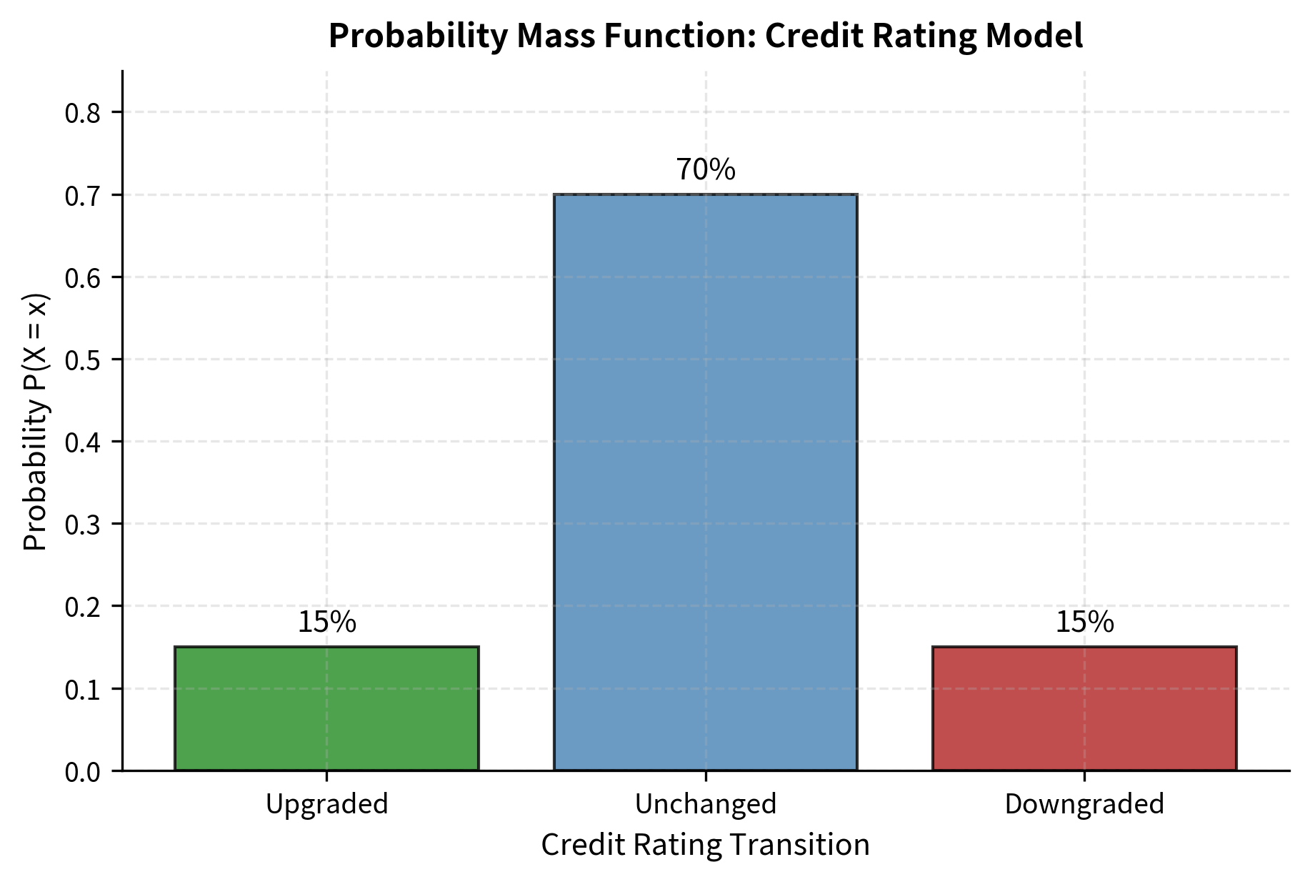
The probabilities sum to 1 because exactly one outcome must occur. This bond will be upgraded, unchanged, or downgraded.there's no other possibility. This summing-to-one requirement is not merely a convention; it follows directly from the Kolmogorov axioms applied to the exhaustive list of mutually exclusive outcomes.
Continuous Random Variables
Financial quantities like returns, prices, and interest rates can take any value within a range, making them continuous random variables. The continuity here refers to the mathematical property that between any two possible values, there are infinitely many other possible values. For continuous variables, we cannot assign probability to individual points because there are uncountably many. Instead, we use probability density functions.
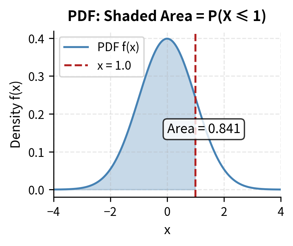
For a continuous random variable , the probability density function (PDF) gives the relative likelihood of values near . The probability that falls in an interval is the area under the density curve: .
The PDF represents a fundamentally different concept than the PMF. Rather than giving the probability of exact values (which is zero for continuous variables), the PDF describes how probability is spread across the continuum of possible values. Higher density means probability is more concentrated in that region, while lower density means probability is more dispersed. The integral formula captures this: to find the probability of landing in an interval, we accumulate (integrate) the density across that interval.
The density itself is not a probability.it can exceed 1 for concentrated distributions. Only when we integrate over an interval do we obtain a probability, which is always between 0 and 1. This distinction often confuses newcomers to probability theory. Think of density as a rate of probability per unit length. A density of 2 at some point doesn't mean probability 2, but rather that probability is accumulating twice as fast near that point compared to a density of 1.
The Cumulative Distribution Function
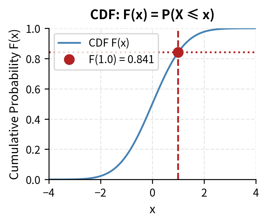
Both discrete and continuous random variables have cumulative distribution functions, providing a unified way to describe probability distributions. The CDF answers the running question "what's the probability of being less than or equal to this value?" as we move along the number line.
The cumulative distribution function (CDF) of a random variable is:
where:
- : CDF evaluated at , giving a probability between 0 and 1
- : probability that takes a value less than or equal to
- As , (impossible to be below all values)
- As , (certain to be below infinity)
The CDF provides a universal framework that works identically for discrete and continuous random variables. This universality makes it valuable for theoretical work and for computing probabilities of intervals: . The CDF always starts at 0 for sufficiently negative values because nothing can be less than negative infinity, increases monotonically as we move right while accumulating more probability, and approaches 1 for large values as it eventually includes all possible outcomes.
The CDF starts at 0 for very negative values and increases to 1 for large values. For continuous distributions, the density is the derivative of the CDF: . This relationship reveals the deep connection between the two representations. The PDF tells us the instantaneous rate at which probability accumulates, while the CDF tells us the total probability accumulated up to each point.
Key Probability Distributions in Finance
Certain probability distributions appear repeatedly in quantitative finance, and each encodes specific assumptions about how uncertainty manifests. Understanding their properties helps you recognize when to apply each one and interpret model outputs correctly. Choosing the right distribution is a fundamental modeling decision.
The Normal Distribution
The normal (Gaussian) distribution dominates financial modeling due to the Central Limit Theorem: sums of many independent random variables tend toward normality regardless of their individual distributions. Since returns aggregate countless buy and sell decisions, they often resemble normal distributions, at least approximately. This mathematical result explains why the normal distribution appears across so many domains: any quantity that results from the combination of many small, independent influences tends toward normality.
A normal random variable has density:
where:
- : probability density at value , representing the relative likelihood of observing a value near
- : mean (center) of the distribution, where the peak occurs
- : standard deviation (spread), controlling the width of the bell curve
- : variance, the square of the standard deviation
- : exponential function ( raised to the given power)
- : mathematical constant (≈ 3.14159)
- The term measures how many standard deviations is from the mean, squared and scaled
- The normalization factor ensures the total area under the curve equals 1
The formula's structure reveals important intuition: the exponential of a negative quadratic creates the characteristic bell shape. Values near the mean () make the exponent close to zero, giving high density, while values far from the mean produce large negative exponents, giving near-zero density. The quadratic form ensures symmetric decay on both sides of the mean. This quadratic dependence in the exponent is what distinguishes the normal distribution from other bell-shaped curves: the rate at which density decreases accelerates as you move away from the mean, creating the rapid tail decay that characterizes normal distributions.
The parameters are:
- : Mean, the center of the distribution. In finance, this represents expected return.
- : Variance, measuring spread. Its square root is the standard deviation, often called volatility.
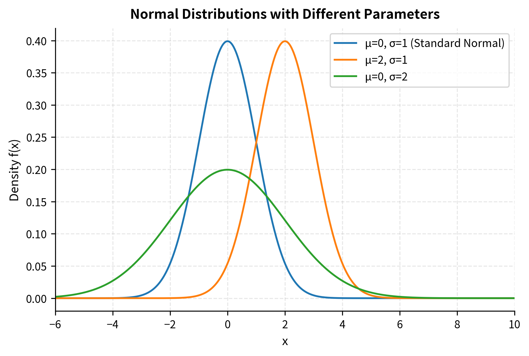
The standard normal distribution (, ) is especially important. Any normal variable can be standardized:
where:
- : standardized random variable (also called z-score)
- : original normal random variable
- : mean of
- : standard deviation of
- : standard normal distribution with mean 0 and variance 1
The standardization formula shifts the distribution so the mean becomes zero (by subtracting ) and scales it so the standard deviation becomes one (by dividing by ). This transformation is a linear rescaling that preserves the shape of the distribution while relocating it to a standard position. The standardized value tells us how many standard deviations the original value lies from its mean.a of 2 means is two standard deviations above average, regardless of what units is measured in.
This transformation allows us to use standard normal tables or functions to compute probabilities for any normal distribution. We only need to tabulate one distribution rather than infinitely many. When a financial analyst computes that a return is "two sigma below average," they're implicitly using this standardization: they've converted the return to a z-score to assess how unusual it is.
The Log-Normal Distribution
While returns may be approximately normal, prices cannot be. A normal distribution allows negative values, but stock prices are always positive. This constraint creates a fundamental modeling challenge. We need a distribution that captures price randomness while respecting the positivity constraint. The log-normal distribution resolves this by modeling the logarithm of the price as normal.
If , then follows a log-normal distribution. This is exactly what happens when returns compound multiplicatively: if each period's return is and log-returns are normal, then the price ratio is log-normal. The log-normal distribution inherits its tractability from the normal distribution while ensuring that prices remain strictly positive, a crucial feature for financial modeling.
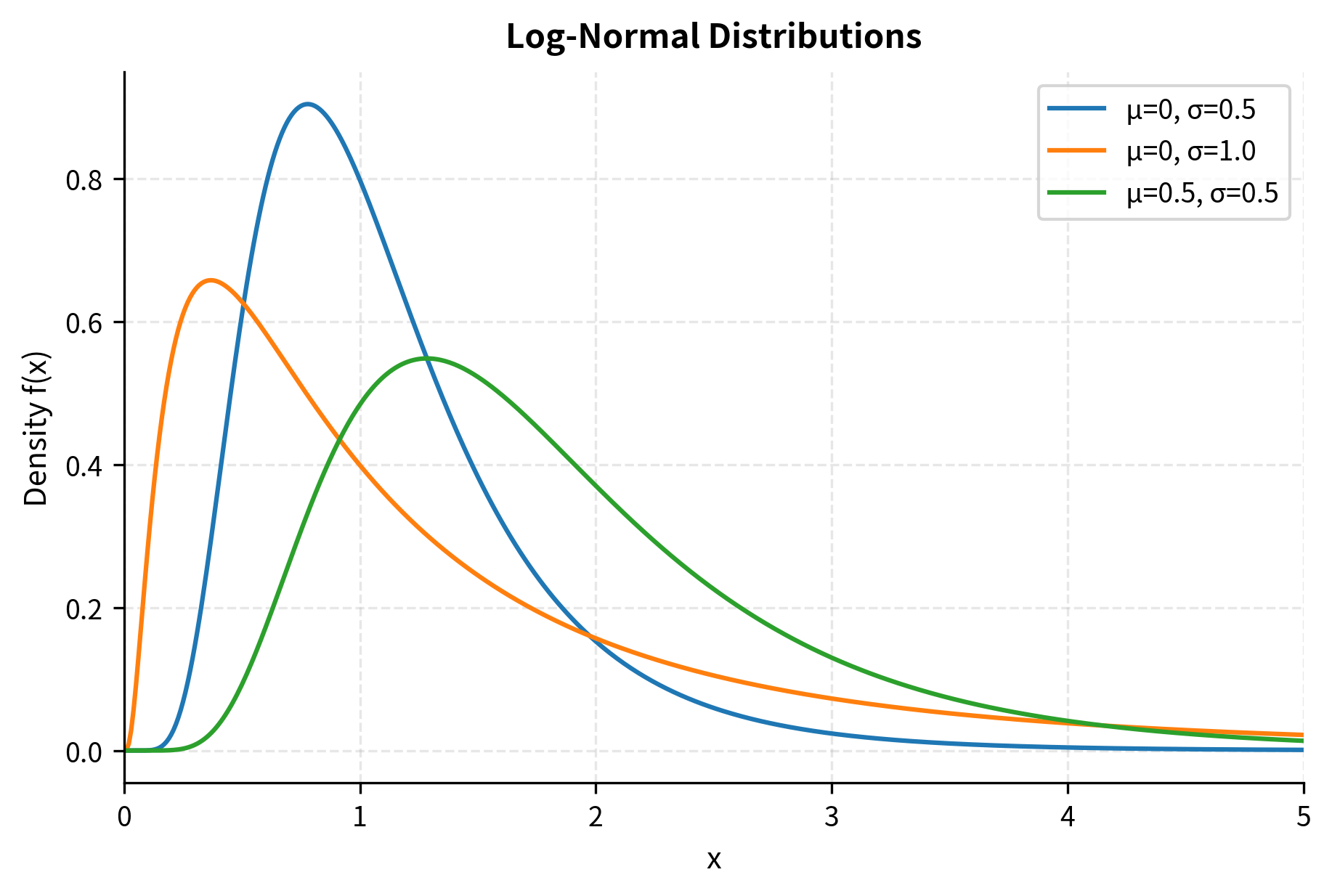
The Black-Scholes option pricing model assumes stock prices follow a log-normal distribution, which ensures prices remain positive while allowing for the mathematical tractability of normal distributions for log-returns. This modeling choice has profound implications: it means log-returns (continuously compounded returns) are normally distributed, and the model permits arbitrarily large percentage gains but bounds losses at 100%. A stock can double, triple, or increase tenfold, but it cannot fall below zero.
Other Important Distributions
Several other distributions appear frequently in quantitative finance, each suited to particular modeling contexts:
- Uniform distribution: Equal probability over an interval. Used for random number generation and some Monte Carlo methods. The uniform distribution represents maximal uncertainty within a bounded range.all values are equally likely.
- Exponential distribution: Models waiting times between events, such as time until the next trade or default. Its "memoryless" property means the probability of an event occurring in the next moment does not depend on how long we have already waited.
- Poisson distribution: Counts events in fixed intervals, like number of trades per minute or credit events per year. Appropriate when events occur randomly and independently at a constant average rate.
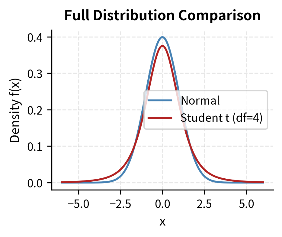
- Student's t-distribution: Similar to normal but with heavier tails, better capturing extreme returns. The t-distribution has a parameter (degrees of freedom) that controls tail heaviness, allowing it to interpolate between normal-like behavior and fat-tailed behavior.
- Chi-squared distribution: Arises in variance estimation and hypothesis testing. Used to quantify uncertainty in volatility estimates and to test whether observed patterns are statistically significant.
Expected Value
The expected value provides a single number summarizing the "center" or "average outcome" of a random variable. It's the theoretical mean you would observe if you could repeat the random experiment infinitely many times. This concept bridges probability theory and practical decision-making: when facing uncertainty, the expected value provides a natural way to summarize what we anticipate on average.
For a discrete random variable with PMF , the expected value is:
For a continuous random variable with PDF :
where:
- : expected value (also called expectation or mean) of random variable
- : possible values that can take
- : probability mass function giving for discrete
- : probability density function for continuous
- : sum over all possible values of
- : integral over the entire real line
The expected value is a probability-weighted average. Outcomes with higher probability contribute more to the average than rare outcomes. Each possible value is weighted by its probability (or density), and these weighted values are summed (or integrated). This weighting scheme ensures that likely outcomes dominate the calculation while rare outcomes contribute proportionally to their likelihood.
The parallel structure between the discrete and continuous formulas reflects a deeper unity: in both cases, we're computing a weighted average where the weights come from the probability distribution. The sum becomes an integral when the set of possible values becomes continuous, but the underlying logic remains the same.
Financial Interpretation
In finance, expected value represents the average return you'd earn if you could repeat an investment many times under identical conditions. A stock with 10% expected annual return won't return exactly 10% each year. It might return 25% one year and -5% the next, but over many years, the average approaches 10%. This long-run interpretation connects the mathematical definition to investment intuition.
Consider a simplified binary stock model:
The expected return of 8% doesn't mean we expect an 8% return on any single investment. It means that if we made this investment many times, our average return would converge to 8%. On any individual occasion, we'll experience either a 20% gain or a 10% loss. The 8% never actually occurs. This distinction between expected value and realized value is fundamental to probabilistic thinking.
Properties of Expected Value
Expected value satisfies several useful properties that make it indispensable for financial calculations:
Linearity: For any random variables and and constants :
where:
- : constants (real numbers)
- : random variables (can be dependent or independent)
- : expected value operator
- : linear combination of the random variables
- : the same linear combination applied to the expected values
This property holds even if and are dependent. The expectation "passes through" the linear combination regardless of any relationship between the variables. This is not true for most other summary measures. The variance of a sum, for example, depends critically on the correlation between variables. Linearity makes portfolio expected return calculations straightforward: the expected return of a portfolio is the weighted average of individual expected returns. If you hold 60% stocks with expected return 10% and 40% bonds with expected return 4%, the portfolio expected return is simply , regardless of how stocks and bonds move together.
Expectation of a function: For a function :
where:
- : any function applied to the random variable
- : the function evaluated at a specific value
- : probability mass function (for discrete )
- : probability density function (for continuous )
This result, known as the Law of the Unconscious Statistician (LOTUS), is remarkably useful: to find the expected value of , we don't need to first derive the distribution of .we simply weight by the original distribution of . The name playfully suggests that statisticians apply this formula "unconsciously" without deriving the transformed distribution. This is essential for computing variance, where , and other moments, as well as for pricing derivatives where the payoff is a function of the underlying asset price.
Variance and Standard Deviation
While expected value describes the center of a distribution, it tells us nothing about spread. Two investments might have the same expected return but vastly different risk profiles. Consider two stocks, both with 10% expected return. One might reliably return between 8% and 12%, while the other swings between -30% and +50%. Expected value alone cannot distinguish these dramatically different risk profiles. Variance quantifies this dispersion.
The variance of a random variable is the expected squared deviation from the mean:
where:
- : variance of random variable , measuring the spread or dispersion of values around the mean
- : expected value operator
- : mean of
- : squared deviation from the mean.squaring ensures all deviations contribute positively and emphasizes larger deviations
- : expected value of squared (the "mean of the square")
- : square of the expected value (the "square of the mean")
The standard deviation is , which returns the measure to the original units of .
The definition of variance as expected squared deviation captures a natural idea: we measure how far each outcome lies from the center, square these distances to eliminate signs and emphasize large deviations, then average over all possible outcomes. Squaring serves two purposes: it makes all deviations positive (a return 5% below average should contribute to dispersion just as much as one 5% above), and it penalizes large deviations more heavily than small ones (being 10% off is more than twice as bad as being 5% off, which aligns with risk aversion in finance).
The second formula, , is computationally convenient. It says variance equals the "mean of the square minus the square of the mean." This formula is often easier to apply because it doesn't require centering the data before squaring. We can compute and separately and then combine them.
To see why these formulas are equivalent, expand the definition:
Since , this gives us . The derivation uses linearity of expectation: we can pass the expectation through the sum and pull constants outside, reducing the problem to computing and .
Financial Interpretation
Standard deviation is the standard measure of risk in finance. A stock with 20% annualized volatility (standard deviation of returns) is considered riskier than one with 10% volatility. Under normality, roughly 68% of returns fall within one standard deviation of the mean, and 95% fall within two standard deviations. These percentages provide benchmarks for interpreting volatility: a 20% volatility stock with 10% expected return will, about two-thirds of the time, return between -10% and +30% in a given year.
The 14.7% standard deviation indicates substantial uncertainty around the 8% expected return. This volatility measure helps investors understand the range of outcomes they face and calibrate position sizes appropriately. A risk-averse investor might demand higher expected returns from this volatile investment compared to a more stable alternative.
Properties of Variance
Variance has different properties than expected value, reflecting its role in measuring spread rather than center:
Scaling: , where is a constant multiplier. Doubling your position quadruples the variance. This quadratic scaling means that leverage amplifies risk faster than it amplifies return. This is a critical consideration for leveraged portfolios.
Sum of independent variables: If and are independent:
This result follows from independence: when and are independent, their covariance is zero, eliminating the cross term that would otherwise appear. Independence means knowing the value of one variable provides no information about the other, so their variances add without reinforcement or cancellation.
Sum of dependent variables: In general:
where:
- : variance of the sum of and
- , : individual variances
- : covariance between and
- The factor of 2 arises because when expanding , the cross term appears, and its expectation is
The covariance term is crucial for portfolio risk. If assets are negatively correlated (negative covariance), the portfolio variance is less than the sum of individual variances. This is the mathematical basis for diversification. When one asset falls, the negatively correlated asset tends to rise, partially offsetting the loss. The covariance term quantifies exactly how much this offsetting reduces overall portfolio risk.
Covariance and Correlation
When analyzing multiple assets, we need to understand how they move together. Covariance and correlation quantify this relationship and provide the mathematical foundation for portfolio construction and risk management. A portfolio's risk depends not only on each component's volatility but also on how those components interact.
The covariance between random variables and measures their joint variability:
where:
- : covariance between and
- : mean of
- : mean of
- : product of deviations from respective means
- : expected value of the product
- The units of covariance are the product of the units of and
The covariance definition captures co-movement through the product of deviations. When both and deviate in the same direction from their means.both above or both below.the product is positive. When they deviate in opposite directions, the product is negative. By taking the expected value of this product, covariance measures the average tendency for the variables to move together.
Positive covariance means and tend to move together: when is above its mean, tends to be above its mean too (both deviations have the same sign, so their product is positive). Negative covariance indicates opposite movements (deviations have opposite signs, so their product is negative). Zero covariance suggests no linear relationship. Knowing that is above average provides no systematic information about whether is above or below average.
The equivalence of the two covariance formulas follows from expanding the definition:
The second formula, , often simplifies calculations: it says covariance equals the expected product minus the product of expectations. If and are independent, , so the covariance is zero. Independence implies zero covariance, though the converse is not generally true.
The correlation coefficient normalizes covariance to lie between -1 and 1:
where:
- : correlation coefficient between and (bounded between -1 and 1)
- : covariance between and
- : standard deviation of
- : standard deviation of
- : product of standard deviations, which has the same units as covariance, making dimensionless
Dividing by the product of standard deviations converts covariance to a standardized scale. A correlation of means a perfect positive linear relationship where knowing exactly determines . A correlation of means a perfect negative linear relationship, and means no linear relationship.
Correlation is easier to interpret than covariance because it's unitless and bounded. A correlation of 1 indicates a perfect positive linear relationship, -1 indicates a perfect negative linear relationship, and 0 indicates no linear relationship. The normalization by standard deviations removes the scale dependence that makes covariance hard to interpret. Whether we measure returns in percentages or decimals, in dollars or euros, the correlation remains the same.
The bounds of -1 and 1 follow from the Cauchy-Schwarz inequality, a fundamental result in mathematics. This bound provides a universal scale for comparison: a correlation of 0.8 between stocks A and B means they move together more strongly than if the correlation were 0.5, regardless of what A and B are or how volatile they are individually.
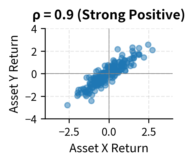
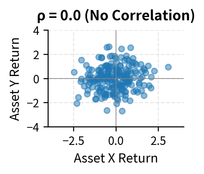
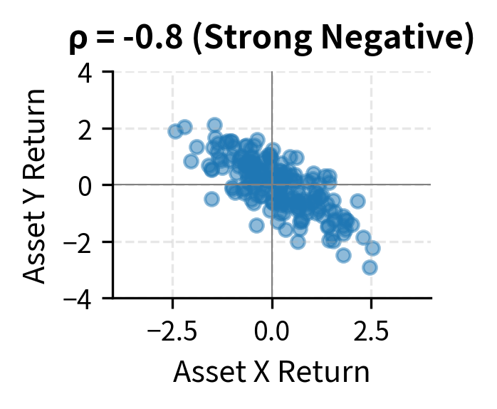
Understanding correlations is essential for portfolio construction. Two assets with low or negative correlation provide diversification benefits: when one falls, the other may rise, reducing overall portfolio volatility. This is the mathematical mechanism behind the old adage "don't put all your eggs in one basket." By combining assets that don't move in lockstep, we can achieve lower portfolio risk than any individual asset offers.
Higher Moments: Skewness and Kurtosis
Mean and variance describe the first two moments of a distribution, but they don't fully characterize it. Two distributions can have identical means and variances yet differ dramatically in their shapes. Higher moments capture asymmetry and tail behavior, which are both critical for understanding financial risk. Investors care not just about average outcomes and volatility but also about the likelihood of extreme gains versus extreme losses.
Skewness
Skewness measures asymmetry around the mean:
where:
- : random variable
- : mean of
- : standard deviation of
- : expected value operator
- The cubic power captures asymmetry: positive deviations contribute positively () while negative deviations contribute negatively (), so a distribution with more extreme positive deviations has positive skewness
- Dividing by makes skewness dimensionless and scale-invariant, allowing comparison across different variables
The choice of the cubic power is not arbitrary. It's the lowest odd power that captures asymmetry. The first power (plain deviations) would sum to zero by definition of the mean. The second power (squared deviations) gives variance but loses sign information. The third power preserves the sign of each deviation, allowing positive and negative extremes to contribute differently. When the distribution has a long right tail with occasional extreme positive values, these large positive cubes dominate and yield positive skewness. A long left tail with extreme negative values yields negative skewness.
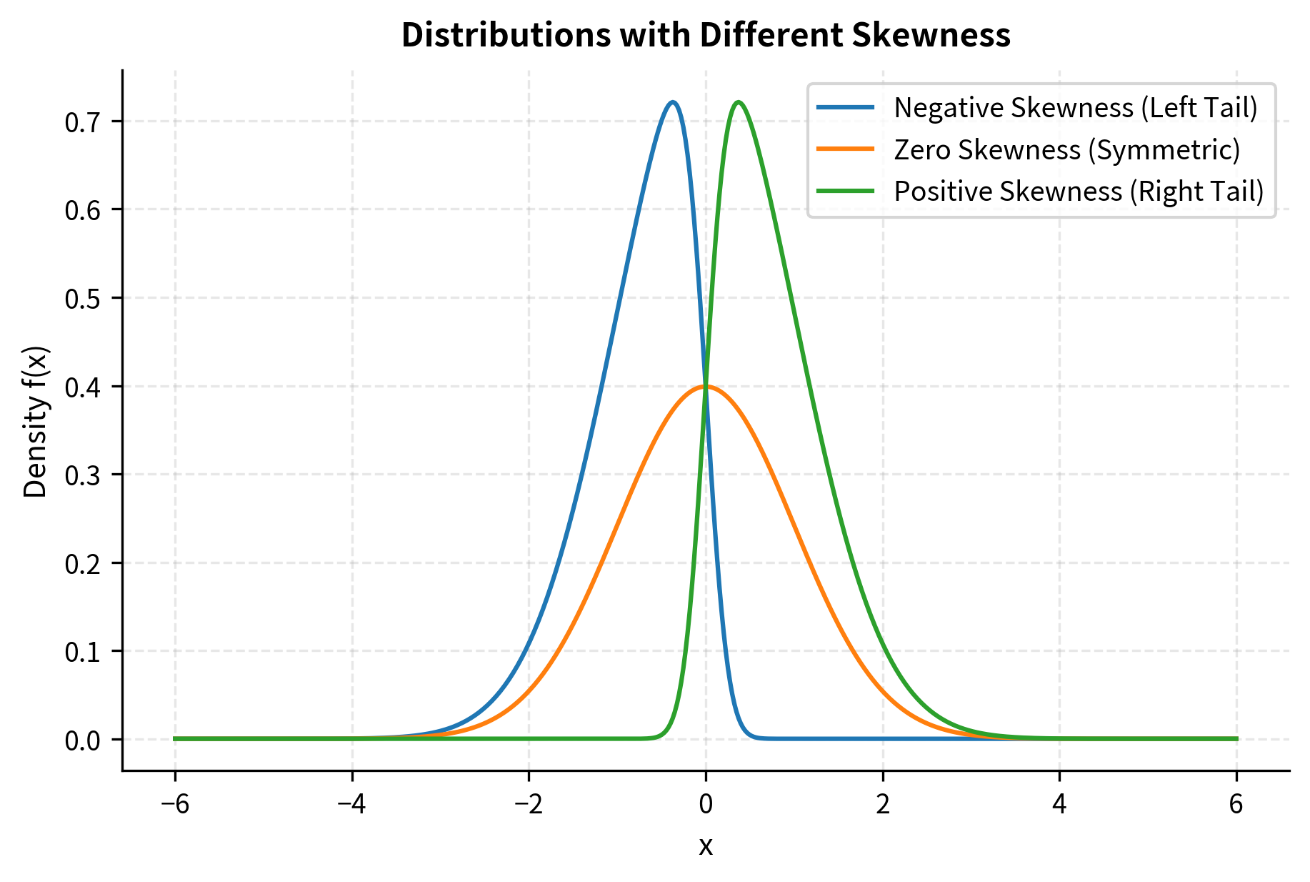
A distribution's skewness reveals the direction and magnitude of its asymmetry:
- Positive skewness: Right tail is longer. There are occasional large positive values. Lottery tickets exhibit positive skewness, with many small losses and rare large gains.
- Negative skewness: Left tail is longer. Occasional large negative values occur. Equity returns often show negative skewness, with gradual gains punctuated by sharp crashes.
- Zero skewness: Symmetric, like the normal distribution.
Investors typically dislike negative skewness. Given two investments with identical mean and variance, most would prefer the one with positive skewness because occasional large gains are more appealing than occasional large losses. This preference reflects fundamental human psychology. Losses loom larger than equivalent gains, a phenomenon documented extensively in behavioral finance.
Kurtosis
Kurtosis measures the heaviness of distribution tails:
where:
- : random variable
- : mean of
- : standard deviation of
- The fourth power emphasizes extreme deviations because raising to the fourth power magnifies large values much more than small ones (e.g., but ), making kurtosis highly sensitive to tail behavior
- Unlike the cubic power in skewness, the fourth power is always positive, so both tails contribute positively
Excess kurtosis subtracts 3 (the kurtosis of a normal distribution): . This normalization sets the normal distribution as the baseline with excess kurtosis of zero.
Kurtosis uses the fourth power of standardized deviations, which dramatically amplifies extreme values. While squaring a deviation of 4 gives 16, raising it to the fourth power gives 256. This sensitivity to outliers is precisely what makes kurtosis useful for detecting fat tails. It picks up the signal from rare but extreme events that other measures might miss. The fourth power, being even, treats positive and negative extremes equally, measuring total tail heaviness rather than asymmetry.
Kurtosis captures the probability of extreme values:
- Excess kurtosis > 0 (leptokurtic): Heavier tails than normal. Extreme events are more likely. Financial returns typically exhibit positive excess kurtosis.
- Excess kurtosis = 0 (mesokurtic): Normal distribution.
- Excess kurtosis < 0 (platykurtic): Lighter tails than normal. Extreme events are less likely.
The fact that financial returns have "fat tails" (positive excess kurtosis) is one of the most important empirical findings in finance. Events that should be extremely rare under normality (such as a 20-standard-deviation move) occur far more frequently than the normal distribution predicts. The 2008 financial crisis and 2020 COVID crash illustrated this dramatically, when "once-in-a-century" moves happened multiple times.
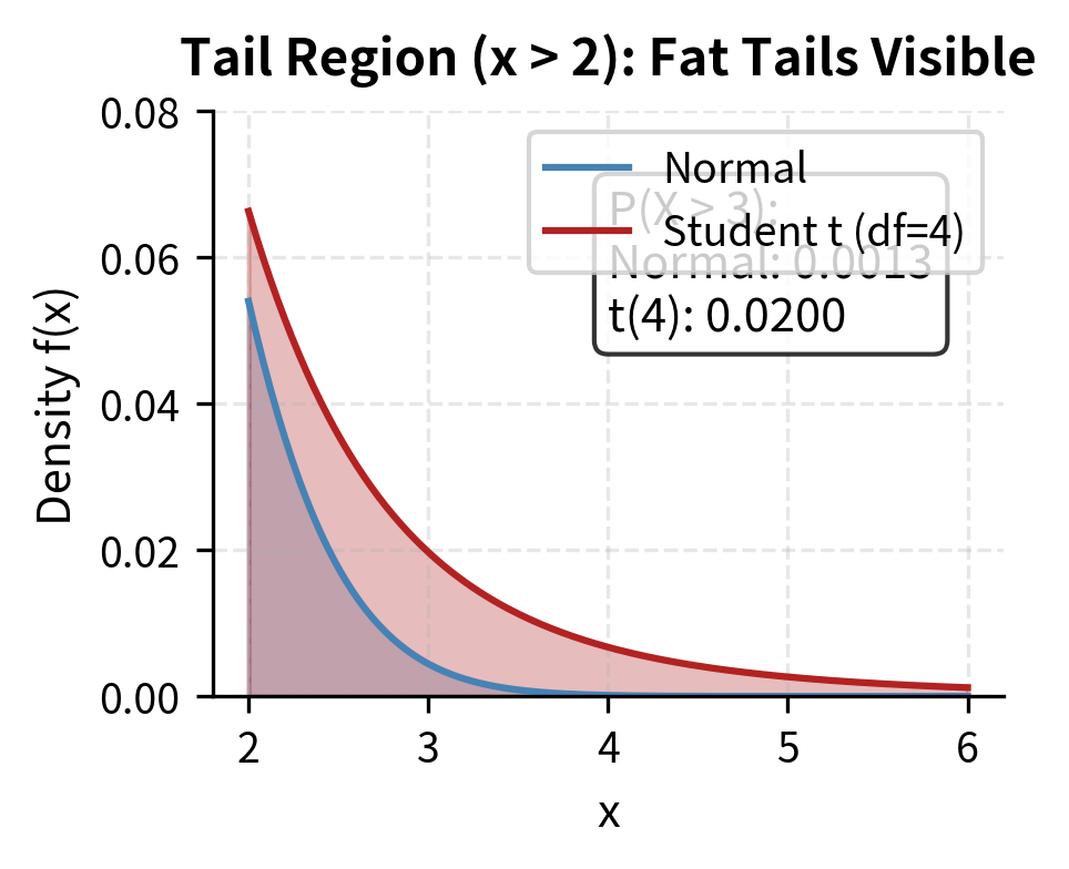
At x = 3, the t-distribution with 4 degrees of freedom has about 15 times the one-tail probability of the normal distribution. This matters enormously for risk management.underestimating tail risk can lead to catastrophic losses. A model that assumes normality might report a near-zero probability of a 4-sigma loss, while the true probability under fat tails is substantially higher.
Conditional Probability
Conditional probability answers the question: "Given that event occurred, what's the probability of event ?" This concept is essential in finance, where we constantly update beliefs based on new information. Markets incorporate news continuously, so our probability assessments must evolve accordingly.
The conditional probability of given is:
where:
- : probability of event occurring given that event has occurred
- : probability that both and occur (joint probability)
- : probability of event (must be greater than 0) The formula captures a simple idea: among all the outcomes where occurred, what fraction also had occur? The denominator restricts our attention to the -world, and the numerator counts the favorable outcomes within that world.
The conditional probability formula implements a natural idea: conditioning on means restricting our universe of possibilities to only those outcomes where occurred. Within this restricted universe, we ask what fraction of outcomes also satisfy . The denominator represents the size of this restricted universe, while the numerator represents the portion where both conditions hold.
The formula says: to find the probability of given , we restrict attention to outcomes where occurred (the denominator) and count the fraction where also occurred (the numerator). This restriction operation is the essence of conditioning: we're not computing probability over the entire sample space but only over the subset where holds.
Financial Example: Credit Risk
Suppose we're analyzing a corporate bond portfolio. Define:
- = bond defaults within one year
- = bond is rated BB (below investment grade)
If 5% of the portfolio are BB-rated bonds, 1% of all bonds default, and 0.3% of bonds are both BB-rated and default, then:
where:
- : probability of default given the bond is BB-rated
- : probability a bond is both BB-rated and defaults (0.3%)
- : probability a bond is BB-rated (5%)
BB-rated bonds have a 6% default probability, compared to 1% for the overall portfolio. This conditional probability helps in setting appropriate credit spreads. A BB-rated bond should offer a higher yield to compensate for this elevated default risk. The calculation also illustrates how conditioning on information, specifically the rating, dramatically changes our probability assessment.
Independence
Two events are independent if knowing that one occurred tells us nothing about the other. Independence is a useful simplifying assumption that, when valid, greatly simplifies probability calculations.
Events and are independent if and only if:
where:
- : learning occurred doesn't change the probability of
- : the joint probability factors into the product of marginals
The two conditions are equivalent: substituting the conditional probability formula into the first condition and multiplying both sides by yields the second.
The first characterization captures the intuitive meaning of independence: observing provides no information about , so our probability assessment for remains unchanged. The second characterization, the multiplication rule, provides a computational criterion: if the joint probability equals the product of marginal probabilities, the events are independent.
Independence is a powerful simplifying assumption. If daily returns are independent (which they approximately are for many assets), we can compute multi-day probabilities by multiplying single-day probabilities. However, real markets exhibit dependencies, especially during crises when correlations spike. The independence assumption should always be verified rather than assumed blindly.
Bayes' Theorem
Bayes' Theorem provides a systematic method for updating probabilities when new information arrives, establishing the mathematical basis for learning from data and adapting beliefs. These skills are essential in finance, where conditions change constantly.
where:
- : posterior probability of given evidence
- : likelihood of observing if is true
- : prior probability of before observing
- : marginal probability of (normalizing constant)
In words: the probability of given equals the probability of given , times the prior probability of , divided by the probability of .
Bayes' Theorem follows directly from the definition of conditional probability applied twice. Starting from and noting that (by rearranging the conditional probability definition for given ), we obtain the theorem. Despite this simple derivation, the theorem has important implications for reasoning under uncertainty.
The components have specific names that reflect their roles in the updating process:
- : Prior probability, representing our belief about before observing
- : Likelihood, measuring how probable the evidence is if is true
- : Posterior probability, representing our updated belief about after observing
- : Evidence probability, which serves as a normalizing constant
The theorem describes rational belief revision: we start with a prior belief, observe evidence, assess how likely that evidence would be under different hypotheses (the likelihoods), and combine these to form a posterior belief. The posterior then becomes the prior for the next round of updating as more evidence arrives.
Worked Example: Updating Default Probabilities
A bank is evaluating a corporate borrower. Based on the firm's industry and size, the bank initially estimates a 3% probability of default within one year. This is the prior probability.
The bank then receives the firm's quarterly financial statements showing deteriorating profit margins. Historical data shows:
- 40% of companies that eventually defaulted showed deteriorating margins in their last year
- 10% of companies that did not default showed deteriorating margins
The bank wants to update its default probability given this new information.
Step 1: Define events
- = company defaults within one year
- = company shows deteriorating margins
Step 2: List known probabilities
- (prior default probability)
- (prior probability of no default)
- (likelihood of margin deterioration given default)
- (likelihood of margin deterioration given no default)
Step 3: Calculate using the law of total probability
Before applying Bayes' Theorem, we need the total probability of observing deteriorating margins, regardless of whether default occurs. The law of total probability provides this by considering all mutually exclusive ways the evidence could arise:
where:
- : total probability of observing deteriorating margins
- : probability of deteriorating margins given the company defaults
- : prior probability of default
- : probability of deteriorating margins given no default
- : probability of no default
This formula works because every company either defaults or doesn't, so we can decompose the probability of deteriorating margins into these two mutually exclusive cases. We weight each conditional probability by the probability of that case occurring. The law of total probability essentially averages the conditional probabilities, weighted by the probability of each conditioning event.
Step 4: Apply Bayes' Theorem
Now we have all the ingredients to compute the posterior probability:
where:
- : posterior probability of default given deteriorating margins (what we want to find)
- : likelihood of deteriorating margins among defaulting companies (0.40)
- : prior default probability (0.03)
- : probability of deteriorating margins (calculated in Step 3)
The numerator represents the probability of both defaulting and showing deteriorating margins. The denominator normalizes this by dividing by the total probability of the evidence.
The deteriorating margins more than tripled our assessed default probability from 3% to about 11%. This updated probability should inform lending decisions, pricing, and reserve requirements. The magnitude of this update reflects both the strength of the evidence, since deteriorating margins are much more common among defaulters, and the prior belief that default was already considered unlikely.
Visualizing Bayes' Theorem
The following visualization shows how the prior probability updates to the posterior as we incorporate new evidence.

Practical Implementation: Simulating Returns and Risk
This section brings together the concepts from this chapter by simulating stock returns and computing risk measures. This exercise demonstrates how probability distributions translate to financial risk analysis.
Simulating Daily Returns
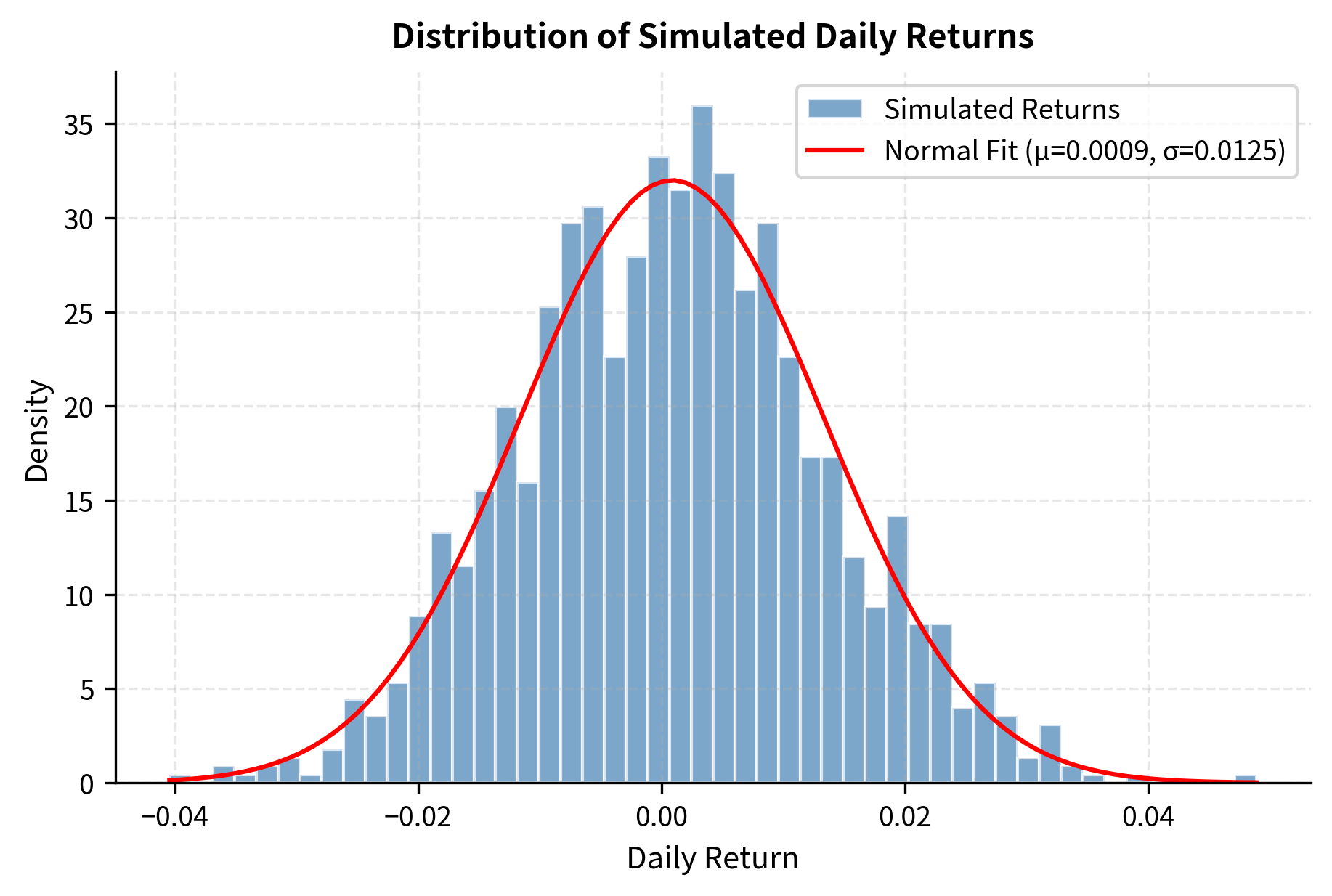
We'll simulate returns using the normal distribution, a common assumption in finance, and compute key statistics.
Computing Sample Statistics
Now we calculate the sample mean, standard deviation, skewness, and kurtosis.
The sample statistics closely match our target parameters, with the annualized mean near 10% and volatility near 20%. The slight deviations illustrate sampling variability. Even with 1,260 observations, estimates aren't perfectly precise. The near-zero skewness and excess kurtosis confirm our simulated returns follow a normal distribution, as expected from our simulation design.
Visualizing the Return Distribution
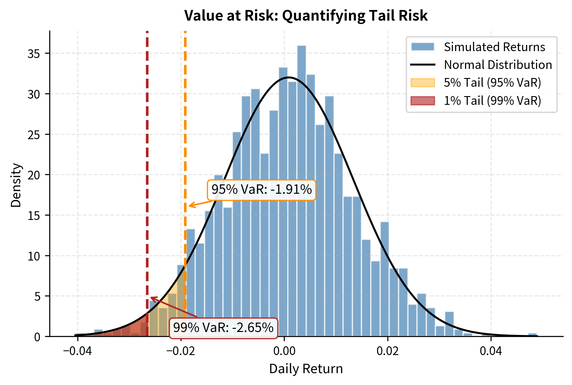
Computing Value at Risk
Value at Risk (VaR) is a common risk measure that answers: "What's the worst loss we'd expect with 95% (or 99%) confidence?" We compute VaR using the percentile of the return distribution.
The 95% VaR of approximately -1.9% means we expect daily losses to exceed this threshold only 5% of the time (roughly once per month of trading). The 99% VaR of about -2.8% represents more extreme tail risk and is exceeded only 1% of the time.
Historical VaR directly uses the percentile of past returns. Parametric VaR assumes a normal distribution and calculates the percentile analytically. When returns are truly normal, as in our simulation, both methods give similar results. For real market data with fat tails, historical VaR is often more conservative.
Converting Price Path from Returns
Starting from an initial price, we can construct a price path using cumulative returns.
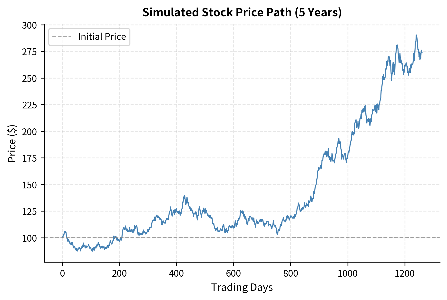
The simulated price path demonstrates the random walk nature of stock prices under our model assumptions. The final price reflects the cumulative effect of daily returns, with the annualized return reasonably close to our 10% target parameter. The path shows typical stock behavior.periods of gains and losses, with an overall upward drift reflecting positive expected returns.
Key Parameters
The key parameters for simulating and analyzing financial returns are:
- annual_return: Expected annual return (e.g., 10%). Determines the drift of the price process and the center of the return distribution.
- annual_volatility: Annualized standard deviation of returns (e.g., 20%). Controls the dispersion and risk of the simulated returns.
- trading_days: Number of trading days per year (typically 252). Used to convert between daily and annual parameters.
- confidence_level: For VaR calculations, typically 95% or 99%. Higher confidence means more conservative risk estimates.
- initial_price: Starting price for the simulation. All subsequent prices are computed relative to this value.
Limitations and Impact
Probability theory provides powerful tools for financial modeling, but practitioners must understand its limitations.
The assumption of known, stable probability distributions rarely holds perfectly in financial markets. Market regimes shift, causing parameters like volatility and correlation to change over time. Models that work during calm markets may fail during crises. The 2008 financial crisis saw correlations between asset classes spike toward 1, precisely when diversification was most needed. Models calibrated on historical data couldn't anticipate this regime shift because the past distribution was no longer representative of the present.
Fat tails present another fundamental challenge. Real financial returns exhibit excess kurtosis, meaning extreme events occur far more frequently than normal distributions predict. A "25-sigma event" that should happen once every years under normality can occur far more frequently in real markets. Risk models that assume normality systematically underestimate the probability of market crashes, leading to inadequate capital reserves and risk limits. This contributed to the 2008 crisis, where many financial institutions held positions that were "safe" according to normal-distribution-based models but proved catastrophic when fat tails materialized.
The gap between sample statistics and true parameters also matters. With finite data, our estimates of means, variances, and correlations contain sampling error. Optimization procedures that treat estimated parameters as true values can generate portfolios that overfit to noise and perform poorly out of sample. This problem is especially severe for expected returns, which require long histories to estimate precisely.
Despite these limitations, probability theory has improved finance significantly. It enables consistent, quantitative risk assessment across diverse assets. Value at Risk, while imperfect, provides a common language for risk limits and capital allocation. Option pricing theory, built on probability distributions of future prices, enabled the multi-trillion-dollar derivatives market. Portfolio optimization, grounded in expected returns and covariances, guides trillions in institutional assets.
The key is using these tools while remaining aware of their assumptions. Supplement parametric models with stress tests. Use longer-tailed distributions when appropriate. Update beliefs as new data arrives, following Bayes' theorem. All models are approximations: useful, but not reality.
Summary
This chapter covered the probability theory foundations essential for quantitative finance.
We began with the formal framework of sample spaces, events, and the Kolmogorov axioms that define valid probability measures. Random variables.both discrete and continuous.map outcomes to numbers, enabling mathematical analysis through probability mass and density functions.
Expected value provides a probability-weighted average, representing the theoretical mean outcome. Variance measures dispersion around this mean, with standard deviation serving as the primary measure of risk in finance. Higher moments (skewness and kurtosis) capture asymmetry and tail behavior, revealing patterns that mean and variance miss.
Conditional probability quantifies how learning new information updates our beliefs. Bayes' Theorem formalizes this updating process, providing a systematic method for incorporating evidence. The credit risk example demonstrated how new financial data can significantly revise default probability estimates.
Key distributions in finance include the normal distribution for returns and the log-normal distribution for prices. However, real returns exhibit fat tails (excess kurtosis) and often negative skewness. These departures from normality matter for risk management.
The practical simulation tied these concepts together: generating returns from probability distributions, computing sample statistics, calculating risk measures like Value at Risk, and constructing price paths. These techniques provide the computational foundation for more advanced quantitative methods.
With these probability foundations, you can tackle portfolio theory, time series analysis, and derivative pricing in the chapters ahead. Each builds directly on the concepts of distributions, expected values, and conditional probabilities introduced here.
Quiz
Ready to test your understanding? Take this quick quiz to reinforce what you've learned about probability theory fundamentals.

Comments