

Master vectors, matrices, and decompositions for portfolio optimization, risk analysis, and factor models. Essential math foundations for quant finance.
Choose your expertise level to adjust how many terms are explained. Beginners see more tooltips, experts see fewer to maintain reading flow. Hover over underlined terms for instant definitions.
Linear Algebra for Quantitative Finance
Linear algebra forms the mathematical backbone of quantitative finance. Every portfolio optimization, risk calculation, and factor model you encounter relies on vectors and matrices to represent assets, returns, and their relationships. Computing portfolio risk involves matrix multiplication. Identifying the key drivers of market movements means finding eigenvectors of a covariance matrix. When you hedge a derivatives book, you're solving a system of linear equations.
This chapter builds your fluency in linear algebra with a constant eye toward financial applications. We start with vectors and matrices, showing how they naturally represent portfolios and return data. We then tackle systems of linear equations, which appear in hedging problems and arbitrage pricing. Finally, we explore matrix decompositions, the powerful techniques that enable principal component analysis and reveal the hidden structure in financial data.
Vectors in Finance
A vector is an ordered list of numbers. In finance, vectors appear everywhere: asset returns, portfolio weights, and factor exposures. The power of vectors lies in how we can manipulate them mathematically to answer financial questions.
Why do we need vectors rather than simply tracking individual numbers? Consider the alternative: if you manage a portfolio of 500 stocks, you could track 500 separate weight variables and 500 separate return variables. But this approach quickly becomes unwieldy. You'd need to write out 500 terms every time you calculate portfolio return, and any formula involving all assets would span pages. Vectors solve this organizational challenge by packaging related quantities into a single mathematical object that we can manipulate as a unit. This abstraction isn't merely notational convenience; it reveals structure. Operations that would be tedious and error-prone with individual variables become clean and computationally efficient with vectors.
Vector Basics
Consider a portfolio containing three assets. We can represent the weights allocated to each asset as a vector:
where:
- : the portfolio weight vector
- : the fraction of portfolio value allocated to asset
Here means 40% of the portfolio value is in asset 1. The vector lives in (three dimensional real space) because it has three components. Geometrically, each asset corresponds to an axis, and the weight vector points to a specific location in this three-dimensional "asset space." Every possible portfolio allocation corresponds to some point in this space. Portfolio constraints, like requiring weights to sum to one, define surfaces or regions within it.
Similarly, we can represent the returns of these three assets on a given day:
where:
- : the return vector for a single time period
- : the return of asset (expressed as a decimal, so 0.02 = 2%)
This says asset 1 returned 2%, asset 2 lost 1%, and asset 3 gained 1.5%. Notice how naturally this representation captures a snapshot of market behavior: all three returns belong together because they occurred simultaneously, and the vector keeps them organized as a coherent unit.
Vector Operations
The fundamental vector operations translate directly into financial calculations:
Scalar multiplication scales every element by a constant. If you double your position in everything:
Geometrically, scalar multiplication stretches or shrinks the vector without changing its direction. Financially, this corresponds to leveraging or deleveraging a portfolio, maintaining the same relative allocations. A leveraged portfolio with 2x weights has double the exposure to every asset, magnifying both gains and losses proportionally.
Vector addition combines vectors element-wise. If and are returns on consecutive days:
where denotes the return of asset on day .
For small returns, this approximates cumulative returns (the exact formula uses geometric compounding). Vector addition also models combining different portfolios. If two funds each contribute capital, the combined portfolio's weight vector is approximately the sum of the individual weight vectors, scaled by the relative capital contributions.
The Dot Product: Portfolio Returns
The dot product (or inner product) of two vectors is the sum of the products of corresponding elements:
where:
- : the number of assets in the portfolio.
This single number has direct financial meaning: it's the portfolio return. The formula captures exactly what we would compute by hand. Each asset contributes to the portfolio return in proportion to both its individual return and the fraction of capital allocated to it. Asset 1's contribution is its weight times its return, asset 2's contribution is its weight times its return, and so on. The dot product sums these contributions to produce the aggregate portfolio performance.
Why does this work? Consider what happens to a $1 portfolio. The amount invested in asset 1 is $w_1, and this grows to $w_1(1 + r_1). Similarly for each asset. The total portfolio value becomes $\sum w_i(1 + r_i) = $(\sum w_i + \sum w_i r_i). Since weights sum to 1, this equals $(1 + \sum w_i r_i), confirming that the portfolio return is indeed the dot product .
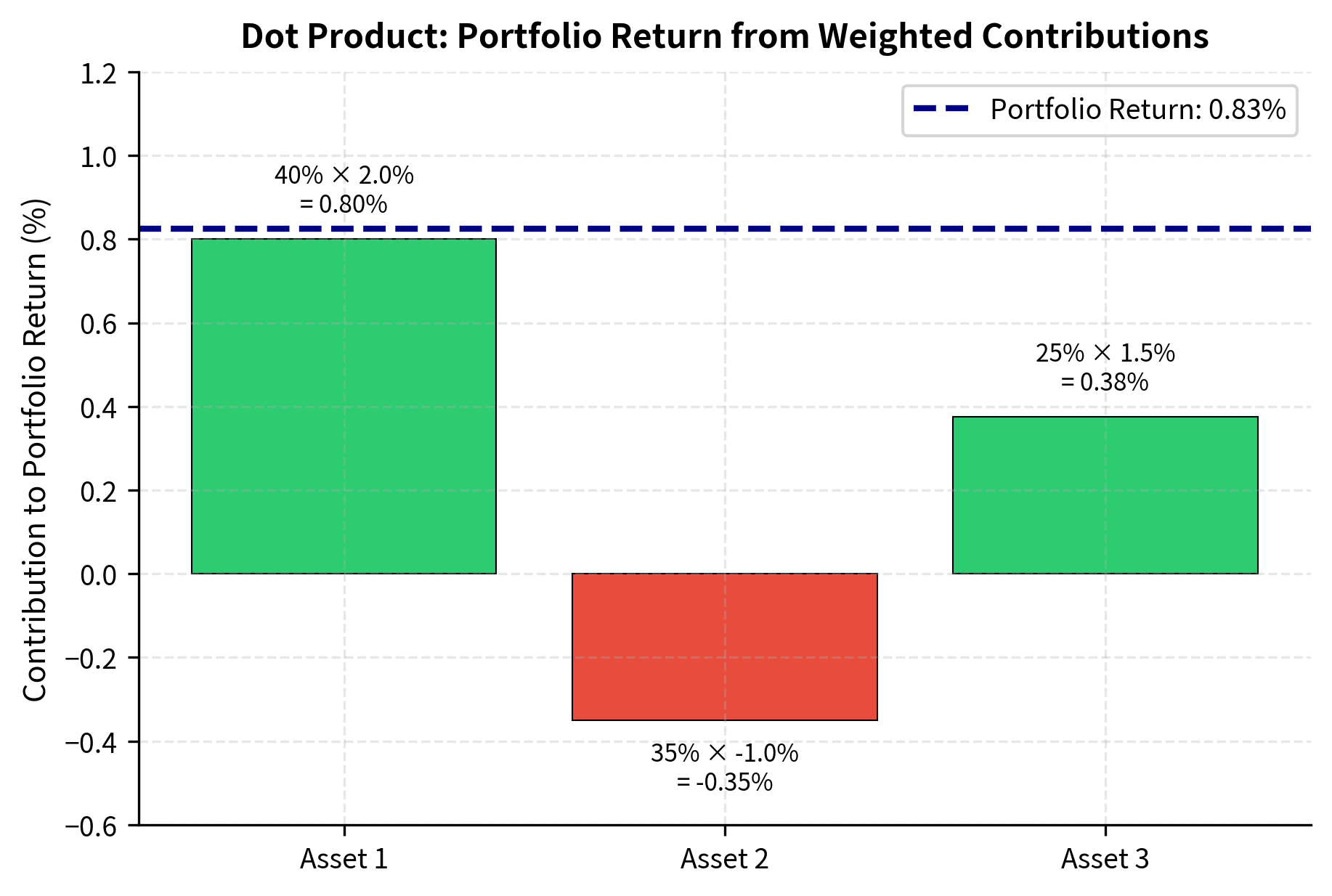
The portfolio earned 0.83% by holding 40% in the 2% gainer, 35% in the 1% loser, and 25% in the 1.5% gainer. This simple calculation.a dot product.underlies virtually every performance calculation in finance.
Vector Norms: Measuring Size
The norm of a vector measures its "size" in various ways. But what does "size" mean for a vector? There's no single answer.different norms capture different notions of magnitude, each useful in different contexts. The most common is the Euclidean norm (or L2 norm):
where:
- : the L2 (Euclidean) norm of vector
- : the -th component of the vector
- : the dimension of the vector
The Euclidean norm corresponds to our intuitive notion of distance: it's the straight-line distance from the origin to the point represented by the vector. In finance, the L2 norm of a return vector relates to volatility. For a vector of deviations from the mean return, the L2 norm (scaled appropriately) gives the standard deviation. This connection between geometric distance and financial risk is one reason the L2 norm appears so frequently in portfolio optimization.
The L1 norm sums absolute values:
The L1 norm measures total "travel distance" if you could only move along coordinate axes, like navigating a city grid where you can only travel along streets, not diagonally through blocks. In portfolio optimization, L1 norms appear in constraints that promote sparse portfolios (holding few assets), as we'll see in later chapters. This is because minimizing the L1 norm of a weight vector tends to push many weights exactly to zero, while the L2 norm spreads weights more evenly across all assets.
The L2 norm of 0.029 represents the Euclidean magnitude of the return vector, which relates to total variability. The L1 norm of 0.06 sums absolute deviations, useful when constructing sparse portfolios. The L∞ norm of 0.02 identifies the largest absolute return, highlighting the most extreme daily movement.
Matrices in Finance
A matrix is a rectangular array of numbers. While vectors represent single entities (one portfolio, one day of returns), matrices represent collections and relationships. These include return history across time, covariances between assets, and transformations between coordinate systems.
The jump from vectors to matrices is conceptually significant. A vector captures one snapshot, such as today's returns or a single portfolio's weights. A matrix captures an entire dataset or a complete description of how quantities relate to each other. When we write down a covariance matrix, we're encoding not just each asset's volatility but every pairwise relationship in the investment universe. When we write down a return matrix, we're capturing the complete history of how multiple assets performed over multiple time periods. This compression of information into a structured rectangular array is what makes quantitative finance computationally tractable.
Matrix Fundamentals
An matrix has rows and columns. In finance, we commonly organize data with rows as time periods and columns as assets:
Here is the return of asset on day . This matrix contains 4 days of returns for 3 assets.
This convention (time as rows, assets as columns) is deliberate and consequential. It means each row represents a complete cross-section of the market at one moment, while each column represents the complete time series of one asset. Extracting a row gives you all assets' returns on a specific day; extracting a column gives you one asset's return history. Most matrix operations in finance align with this convention, so understanding the layout helps you interpret results correctly.
Matrix Multiplication
Matrix multiplication is the workhorse operation of linear algebra. For matrices (size ) and (size ), the product is an matrix where:
where:
- : element in row , column of the result matrix
- : element in row , column of matrix
- : element in row , column of matrix
Each element of the result is a dot product of a row from with a column from .
Each element of the result shows how much the -th row of aligns with the -th column of . In financial terms, when multiplying a return matrix by a weight vector, each resulting element aggregates the weighted contributions of all assets for that time period. You can think of matrix multiplication as performing many dot products simultaneously. The entry of the product answers the question "how does row of the first matrix relate to column of the second?"
This interpretation illuminates why matrix multiplication has the dimensional requirements it does. The dot product requires vectors of equal length, so for each row-column pair to produce a dot product, the row length (number of columns in ) must equal the column length (number of rows in ). The result matrix takes its row count from and its column count from because we compute one number for each possible row-column pairing.
For matrix multiplication to be valid, the number of columns in must equal the number of rows in . The result has the number of rows from and columns from : .
A critical financial application is computing portfolio returns across multiple days. If is a matrix of returns ( days, assets) and is an weight vector, then gives a vector of portfolio returns:
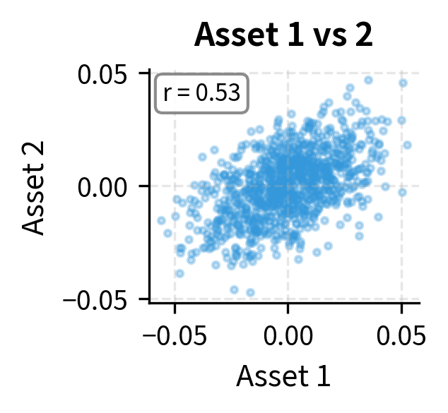
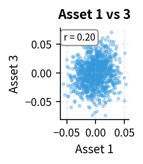
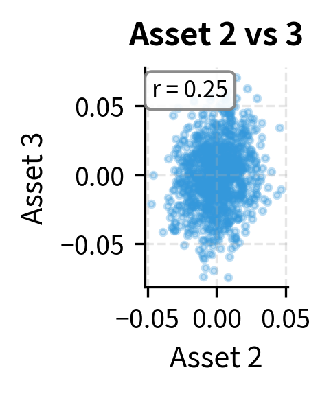
The Covariance Matrix
The covariance matrix captures how assets move together. For assets, it's an symmetric matrix where element is the covariance between assets and :
where:
- : the element of the covariance matrix
- : returns of assets and
- : expected (mean) returns of assets and
- : the expectation operator
The formula shows what covariance measures: we're looking at the product of deviations from the mean. When asset is above its average and asset is also above its average, the product is positive. When both are below average, the product is again positive. But when one is above and the other below, the product is negative. By averaging these products across many observations, covariance tells us whether two assets tend to move together (positive covariance), move oppositely (negative covariance), or move independently (covariance near zero).
The diagonal elements are variances of individual assets. The off-diagonal elements measure co-movement. Positive covariance means assets tend to move together. Negative covariance means they move oppositely.
Portfolio Variance: The Quadratic Form
Portfolio variance demonstrates the power of matrix notation. For a portfolio with weights and asset covariance matrix , the portfolio variance is:
where:
- : the variance of the portfolio's returns
- : the vector of portfolio weights
- : the transpose of (a row vector)
- : the covariance matrix of asset returns
This compact formula packs a lot of computation: it accounts for each asset's variance and all pairwise covariances, weighted by the portfolio allocations. The expression is called a quadratic form because if you expand it, you get a polynomial where each term involves products of two weights.it's quadratic in the portfolio allocations.
Expanding for two assets:
where:
- : the variances of assets 1 and 2
- : the covariance between assets 1 and 2
The first two terms are variance contributions from each asset. The third term involving covariance is why diversification works. When (negative correlation), it reduces portfolio variance. Even when covariance is positive but less than the geometric mean of the variances, diversification still helps by ensuring the portfolio variance is less than the weighted average of individual variances.
The matrix formulation generalizes seamlessly to any number of assets. For 500 stocks, the formula remains (the same compact expression) while the expanded version would require summing 250,500 terms (500 variances plus 124,750 unique covariances, each appearing twice). This is the power of linear algebra notation: it scales effortlessly from toy examples to production systems.
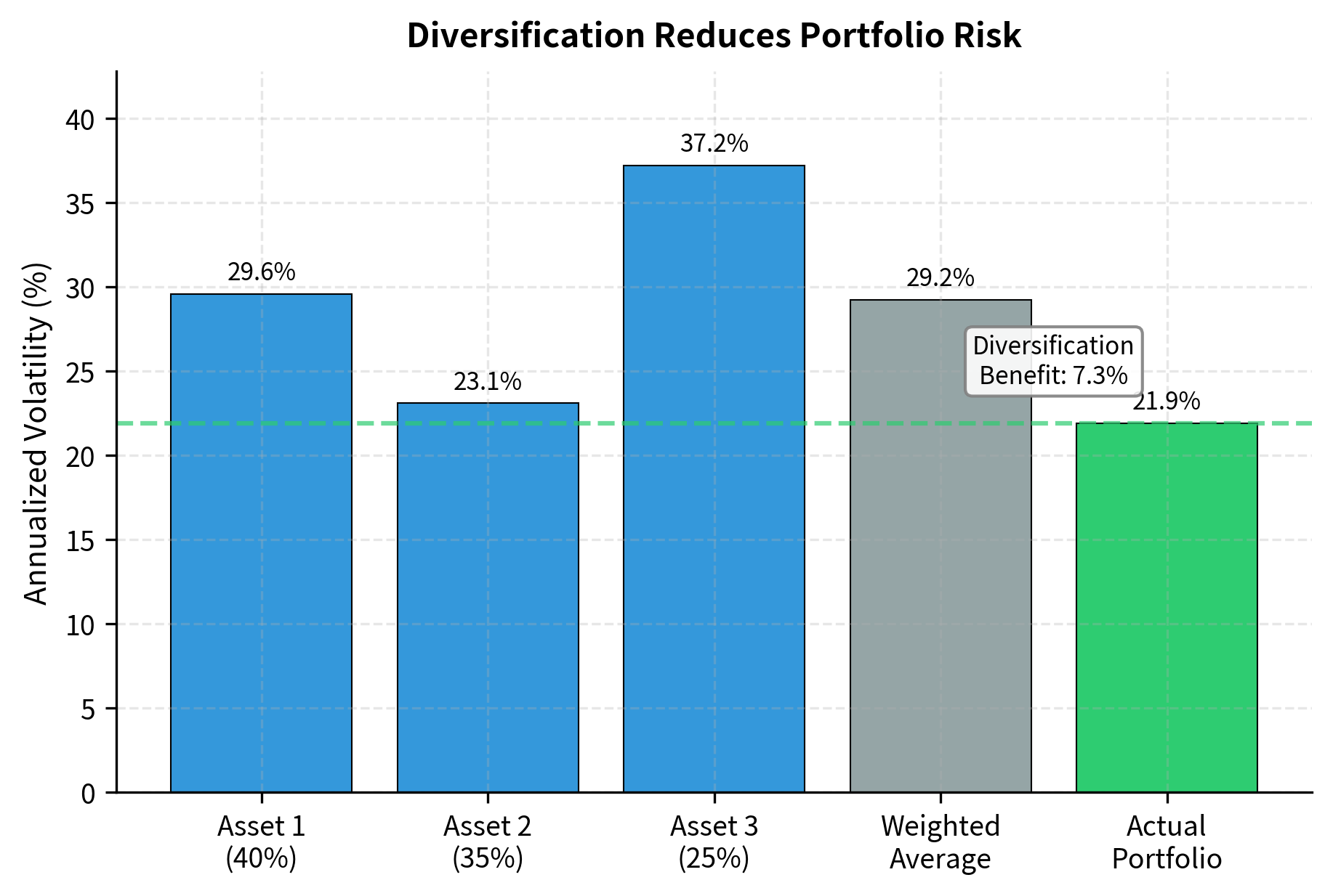
The portfolio volatility is lower than the weighted average of individual volatilities because the assets are imperfectly correlated. This is the mathematical basis of diversification.
Matrix Transpose and Special Matrices
The transpose of matrix , written , flips rows and columns: .
Several special matrix types appear frequently in finance:
- Symmetric matrices: . Covariance matrices are always symmetric. This property reflects a fundamental reality: the covariance between assets A and B must equal the covariance between B and A, since we're measuring the same relationship from both directions.
- Diagonal matrices: Non-zero elements only on the diagonal. Used to represent variance contributions when assets are uncorrelated, or to scale different variables by different amounts.
- Identity matrix: Diagonal matrix with 1s on the diagonal. Acts as the "1" of matrix multiplication: . It's the matrix equivalent of multiplying by one, leaving any matrix unchanged.
- Positive definite matrices: for all non-zero . Valid covariance matrices must be positive semi-definite (allowing zero). This property ensures that no portfolio can have negative variance, a mathematical necessity for any coherent risk measure.
Both properties confirm we have a valid covariance matrix. Symmetry ensures that the covariance between assets A and B equals the covariance between B and A. Positive semi-definiteness guarantees that no portfolio can have negative variance.a mathematical necessity for any coherent risk measure.
Systems of Linear Equations
Many financial problems reduce to solving systems of linear equations. Hedge ratios, factor exposures, and arbitrage pricing all require solving for unknown .
Why is this formulation so ubiquitous? Because linear systems capture the essence of constraints and requirements. In finance, we often face situations where multiple conditions must hold simultaneously. A hedge must neutralize exposure to several risk factors at once, a replicating portfolio must match the payoffs of a target in multiple scenarios, and factor loadings must explain returns across many time periods. Each condition contributes one equation, and the unknowns are the positions or weights we need to determine. Linear algebra provides systematic machinery for finding solutions when they exist and for characterizing what's possible when they don't.
The General Problem
A system of linear equations has the form:
where:
- : the coefficient in equation for unknown
- : the -th unknown variable we're solving for
- : the right-hand side constant of equation
- : the number of equations
- : the number of unknowns
In matrix form: , where is , is , and is .
The matrix encodes the structure of the problem.how each unknown contributes to each equation. Finding means finding the combination of unknowns that simultaneously satisfies all constraints. In financial applications, often represents sensitivities (like Greeks or factor exposures), represents positions or weights we're solving for, and represents target values we want to achieve.
The geometry of linear systems provides useful intuition. Each equation defines a hyperplane in the space of unknowns (a line in 2D, a plane in 3D, and so on). Solving the system means finding the point (or points, or nothing at all) where all these hyperplanes intersect. When there are exactly as many independent equations as unknowns, and the equations aren't contradictory, the hyperplanes intersect at a single point, giving the unique solution.
Matrix Inverses and Solving Square Systems
When is square () and invertible, the solution is . The inverse satisfies .
The inverse matrix "undoes" the transformation represented by . If transforms inputs to outputs, then transforms outputs back to inputs. In the context of our linear system, we know the outputs (, the targets we want to achieve) and need to find the inputs (, the positions that achieve those targets). Multiplying by the inverse reverses the process, revealing the required inputs.
A square matrix is invertible (or non-singular) when its determinant is non-zero, equivalently when its rows (or columns) are linearly independent. Economically, this means the equations provide truly independent constraints. No equation is redundant or contradictory with others.
Application: Factor Replication
Consider replicating a target portfolio's factor exposures using available assets. Suppose you have three assets with known exposures to two factors (market and size), and you want to construct a portfolio with specific target exposures:
We have 3 unknowns (weights) and 3 equations (2 factor constraints + 1 budget constraint). Let's solve:
The solution tells us exactly how to combine the three assets to achieve our target factor profile: market beta of 1 with zero size exposure, while being fully invested.
Application: Delta Hedging
In derivatives trading, you often need to hedge exposure to multiple risk factors. Suppose you hold a portfolio of options and want to eliminate sensitivity to the underlying price (delta) and volatility (vega). You have two hedging instruments available:
We need to short 160 shares of stock and buy 20 options to neutralize both delta and vega exposure. This is precisely the kind of calculation that happens in real-time at trading desks.
Least Squares: Overdetermined Systems
When we have more equations than unknowns (), the system is overdetermined and typically has no exact solution. This happens often in finance. We have many data points (days of returns) but few parameters to estimate (factor exposures).
The least squares solution minimizes the sum of squared residuals:
where:
- : the least squares estimate of
- : the squared L2 norm (sum of squared elements)
- : the residual vector
The solution is given by the normal equations (assuming is invertible):
where:
- : a square matrix that captures the "self-correlation" of the explanatory variables
- : inverts this correlation structure to prevent double-counting
- : correlates the explanatory variables with the target values
When is invertible, the matrix is the Moore-Penrose pseudoinverse of .
Intuitively, least squares finds the that makes as close as possible to in Euclidean distance. The residual vector is orthogonal to the column space of . We've extracted all the signal that can explain. What remains (the residual) lies in a direction that no linear combination of our explanatory variables can reach.
This geometric picture explains why least squares produces the best linear fit. Among all possible values of , the least squares solution generates an that is the orthogonal projection of onto the subspace spanned by the columns of . Orthogonal projection onto a subspace always yields the closest point in that subspace. This is a basic geometric fact. The residual, being orthogonal to the subspace, represents the irreducible error that cannot be explained by our model.
This is exactly what linear regression computes.
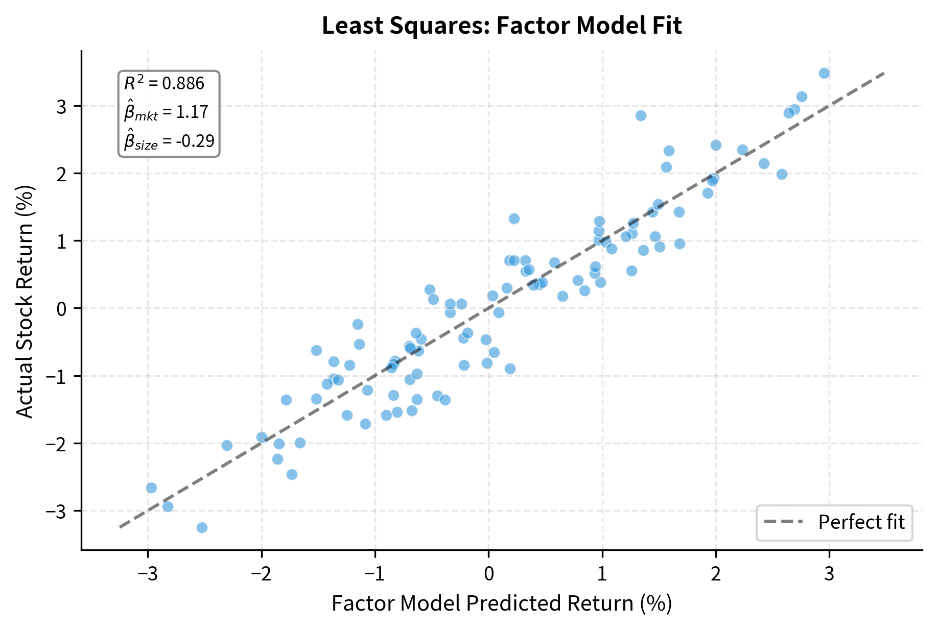
The least squares estimates are close to the true values, with small errors due to the noise in returns. With more data (more days), the estimates would converge to the true values.
Matrix Decompositions
Matrix decompositions break a matrix into simpler components, exposing structure that's hidden in the raw numbers. In quantitative finance, decompositions help us understand risk sources, reduce dimensionality, and improve numerical stability.
Think of decomposition as a kind of mathematical X-ray. A covariance matrix appears as a dense array of numbers, but its eigendecomposition reveals the underlying modes of variation, the basic ways ways in which assets tend to move together. A return matrix might contain hundreds of thousands of numbers, but its singular value decomposition exposes the dominant patterns that generate most of the observed variation. Decompositions transform opaque numerical arrays into interpretable components with clear financial meaning.
Eigenvalue Decomposition
An eigenvalue decomposition expresses a square matrix as:
where:
- : an matrix whose columns are the eigenvectors
- : a diagonal matrix with eigenvalues on the diagonal
- : the inverse of the eigenvector matrix, which "undoes" the coordinate transformation
This decomposition shows that acts as: (1) rotating into the eigenvector coordinate system via , (2) scaling each axis by the corresponding eigenvalue via , and (3) rotating back via . For covariance matrices, we can decompose complex correlations into independent directions of variation.
The power of this decomposition lies in the simplicity of the diagonal matrix . A diagonal matrix just scales each coordinate independently, with no mixing between directions. All the complexity of is absorbed into finding the right coordinate system (the eigenvectors) in which the matrix action becomes simple scaling.
An eigenvector of matrix satisfies , where is the eigenvalue. The matrix simply scales the eigenvector by , without changing its direction. For symmetric matrices like covariance matrices, eigenvectors are orthogonal and eigenvalues are real.
For a covariance matrix, the eigenvectors represent the principal directions of variation in the data, and the eigenvalues represent the variance along each direction. The largest eigenvalue corresponds to the direction of maximum variance. This interpretation makes eigendecomposition indispensable for understanding portfolio risk: the dominant eigenvector shows which combination of assets contributes most to overall portfolio variance.
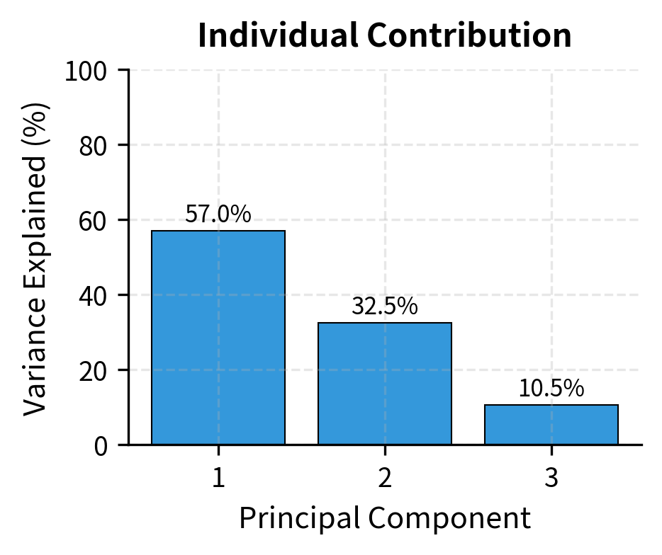
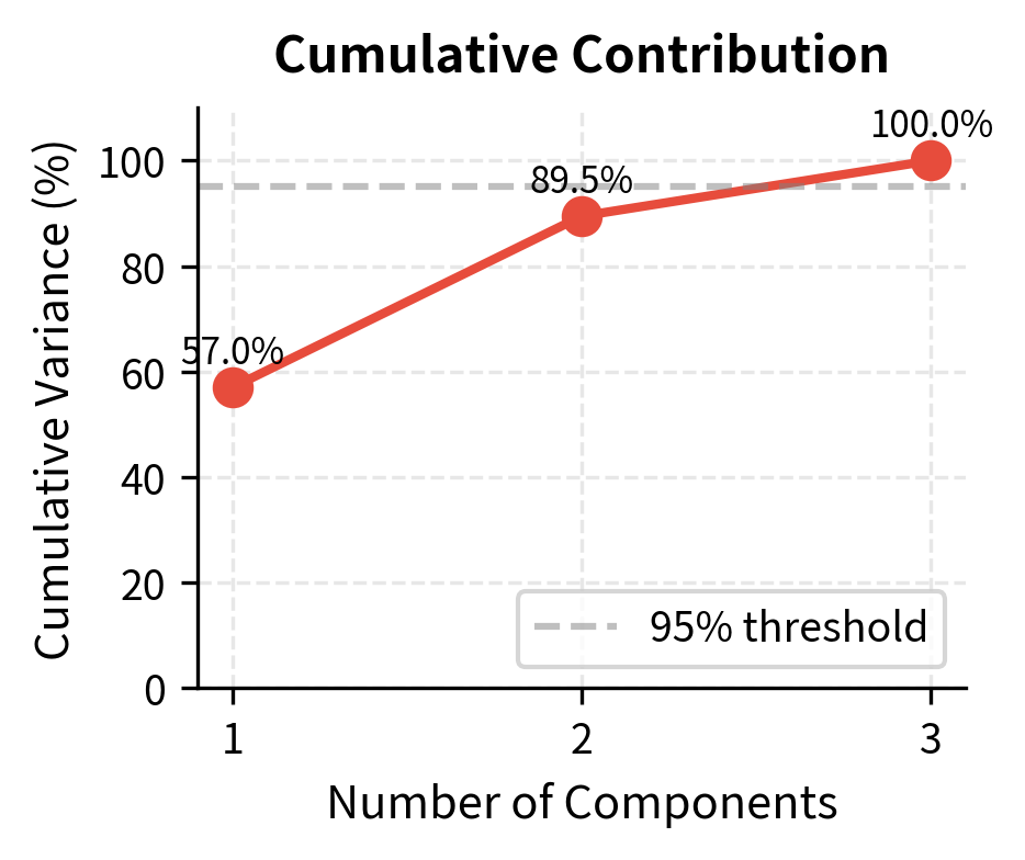
Principal Component Analysis (PCA)
PCA uses eigendecomposition to transform correlated variables into uncorrelated principal components. In finance, PCA identifies the main drivers of asset returns: often, a few factors explain most of the variation in a large universe of assets.
The principal components are projections of the data onto the eigenvectors:
where:
- : the matrix of principal component scores
- : the centered data matrix (each row is an observation, each column is a variable minus its mean)
- : the matrix of eigenvectors (principal component loadings)
Each column of represents a principal component, a new synthetic variable that captures a specific pattern of co-movement in the original data. The first principal component captures the most variance, the second captures the most remaining variance while being uncorrelated with the first, and so on. In finance, these components often correspond to interpretable market factors like overall market direction, sector rotations, or style tilts.
Why does this transformation produce uncorrelated components? The eigenvectors of a symmetric matrix (like a covariance matrix) are orthogonal. They point in perpendicular directions. When we project data onto perpendicular axes, the resulting coordinates are uncorrelated by construction. The eigenvalues tell us how much variance lies along each axis, so ordering by eigenvalue puts the most important component first.
The first principal component typically captures broad market movements.all loadings have the same sign. Later components capture relative value or sector bets, and loadings have mixed signs. This structure emerges naturally from the correlation structure of returns.
PCA in Practice: Interest Rate Curves
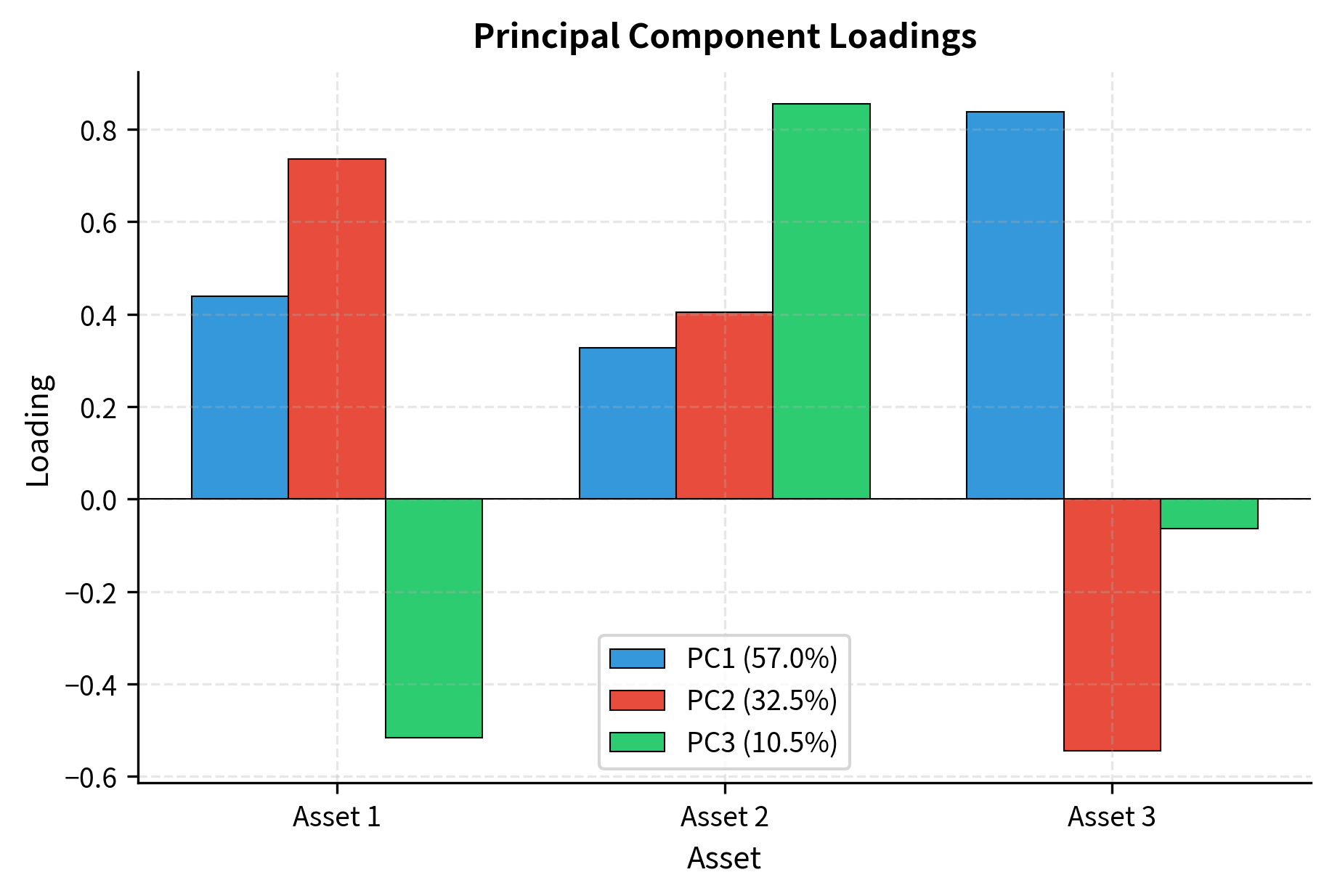
One of the most powerful applications of PCA in finance is analyzing yield curve movements. Interest rates at different maturities are highly correlated, but PCA reveals that three factors explain over 95% of yield curve variation:
- Level (PC1): Parallel shift in the curve. All rates move together.
- Slope (PC2): Steepening or flattening. Short and long rates move in opposite directions.
- Curvature (PC3): Bending. The middle of the curve moves relative to the ends.
This parsimony (three numbers summarizing an entire term structure) shows the value of PCA for dimensionality reduction. Instead of tracking eight or more rates independently, a fixed income trader can focus on level, slope, and curvature exposures.
PC1 shows positive loadings across all maturities, confirming it captures level shifts. PC2 is negative for short maturities and positive for long ones, capturing slope. PC3 has a distinctive "humped" pattern.negative at the ends, positive in the middle.capturing curvature. Bond portfolio managers use these insights to decompose and hedge their interest rate risk.
Singular Value Decomposition (SVD)
While eigendecomposition only applies to square matrices, Singular Value Decomposition works for any matrix. For an matrix :
where:
- : an orthogonal matrix whose columns are the left singular vectors (patterns in the row space, e.g., time patterns)
- : an diagonal matrix with non-negative singular values on the diagonal
- : an orthogonal matrix whose columns are the right singular vectors (patterns in the column space, e.g., asset patterns)
The singular values measure the "importance" of each component. For a return matrix with days as rows and assets as columns, shows when certain patterns occurred, shows which assets participated in each pattern, and shows how strong each pattern was.
The strength of SVD lies in its universality and interpretability. Any matrix, not just square symmetric ones, can be decomposed into rotations and scalings. The singular values are always non-negative and ordered by magnitude, providing a natural ranking of importance. Truncating the SVD by keeping only the largest singular values gives the best low-rank approximation to the original matrix in terms of Frobenius norm, a result known as the Eckart-Young theorem. This makes SVD the mathematical foundation for dimensionality reduction and data compression.
SVD is useful for handling non-square return matrices (different numbers of days vs. assets) and for computing the pseudoinverse used in least squares solutions.
The close match between eigenvalues and σ²/(T-1) confirms the mathematical relationship between SVD and eigendecomposition. The largest singular value corresponds to the dominant pattern in the return matrix, typically the market factor. This relationship is why PCA can be computed efficiently via SVD, which is numerically more stable than computing the eigendecomposition of the covariance matrix directly.
Cholesky Decomposition
For positive definite matrices, including covariance matrices that are strictly positive definite, Cholesky decomposition provides a "square root":
where:
- : a lower triangular matrix (all entries above the diagonal are zero)
- : the transpose of (an upper triangular matrix)
The Cholesky factor is unique for positive definite matrices and can be computed efficiently in operations, half the cost of a general matrix factorization.
where is lower triangular. This is computationally efficient and important for simulating correlated random variables, essential for Monte Carlo methods in derivatives pricing and risk management.
The lower triangular structure of has a clear interpretation in terms of sequential dependence. The first asset's random component depends only on one source of randomness. The second asset depends on the first asset's randomness through correlation, plus its own independent randomness. The third asset depends on both previous assets' randomness plus a third independent source. This cascading structure mirrors how correlated variables can be constructed. Start with independent random variables and mix them according to the correlation structure.
The simulated covariance matrix closely matches the original, confirming that our Cholesky-based sampling correctly reproduces the correlation structure. The lower triangular form of L shows how each asset's random component builds on the previous ones: Asset 1 has independent randomness, Asset 2 combines Asset 1's randomness with its own, and Asset 3 incorporates components from both. This cascading structure is why Cholesky decomposition efficiently generates correlated samples.
The Cholesky decomposition allows us to generate correlated random returns for Monte Carlo simulation. This is essential for pricing path-dependent derivatives and computing Value-at-Risk.
A Complete Example: Minimum Variance Portfolio
Let's bring together the linear algebra concepts to solve a standard portfolio optimization problem: finding the portfolio with minimum variance subject to being fully invested.
The optimization problem is:
subject to:
where is a vector of ones (enforcing that weights sum to 1, meaning the portfolio is fully invested).
This problem asks which portfolio, among all portfolios that invest 100% of capital (no cash, no leverage), which has the smallest variance? The objective function is the quadratic form we encountered earlier, portfolio variance expressed in matrix notation. The constraint is a linear equation requiring weights to sum to unity.
Using Lagrange multipliers, the solution is:
where:
- : the optimal weight vector that minimizes portfolio variance
- : the inverse of the covariance matrix
- The numerator gives "risk-adjusted" weights favoring low-variance and negatively-correlated assets
- The denominator normalizes these weights to sum to 1
The appearance of in the solution formula is typical of quadratic optimization with linear constraints. Intuitively, the inverse covariance matrix reweights assets to account for correlation. An asset that seems low-variance in isolation might contribute more risk than expected if it's highly correlated with other holdings. The inverse covariance matrix adjusts for these interactions, identifying the truly risk-efficient allocation.
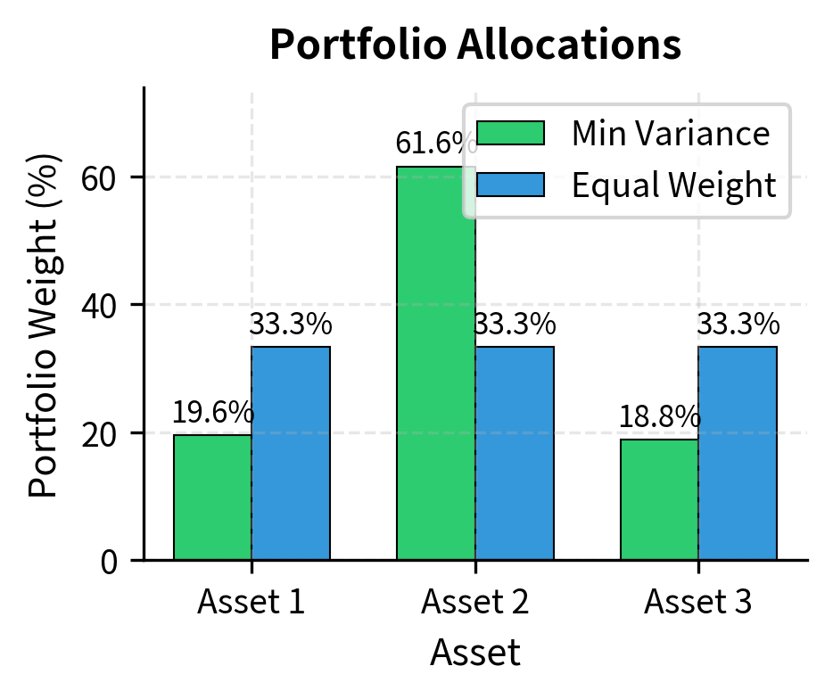
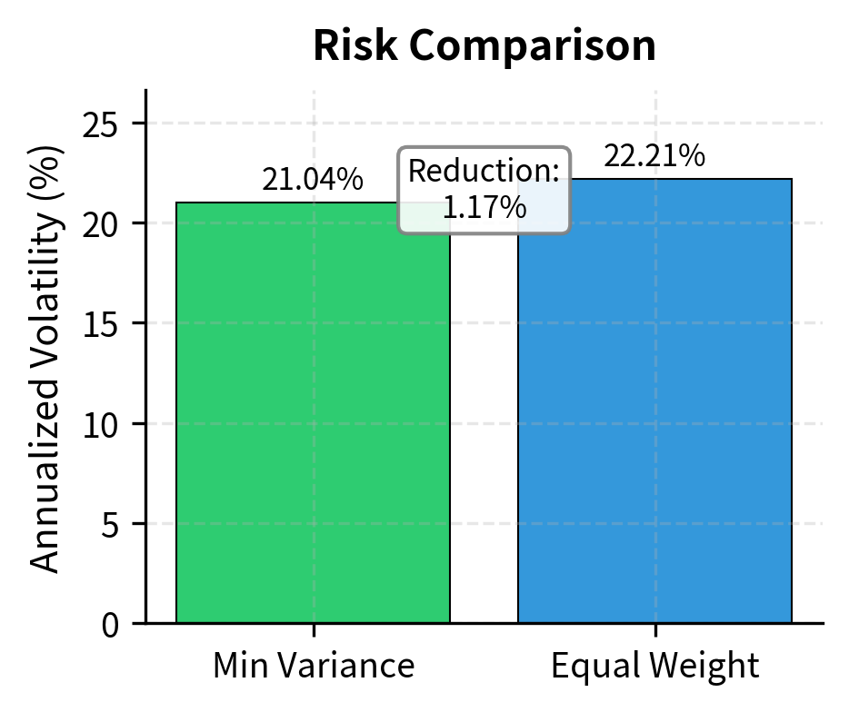
The minimum variance portfolio allocates more to lower-volatility assets and exploits negative or low correlations to reduce overall portfolio risk. Notice that this solution used matrix inversion () and multiple matrix-vector multiplications.fundamental linear algebra operations that power quantitative portfolio construction.
Key Parameters
The key parameters for linear algebra operations in quantitative finance are:
- Portfolio weights (w): The fraction of portfolio value allocated to each asset. Must sum to 1 for a fully invested portfolio.
- Covariance matrix (Σ): Captures variance of individual assets (diagonal) and co-movement between assets (off-diagonal). Must be positive semi-definite.
- Eigenvalues (λ): Represent variance along each principal direction. Larger eigenvalues indicate more important risk factors.
- Eigenvectors (V): Define the principal directions of variation. For covariance matrices, these are orthogonal and reveal underlying factor structure.
- Condition number: Ratio of largest to smallest eigenvalue. High values indicate numerical instability in matrix inversion.
Limitations and Practical Considerations
Linear algebra provides clean solutions, but real-world implementation requires caution around several issues.
Estimation error is the most significant challenge. Covariance matrices estimated from historical data are noisy, especially with many assets relative to the number of observations. A 500-stock universe with 252 days of data means estimating 125,250 covariance parameters from only 126,000 data points, almost one parameter per observation. This leads to unstable matrix inverses and portfolio weights that swing wildly with small changes in the data. Practitioners address this through shrinkage estimators, factor models, and regularization techniques that we'll explore in later chapters.
Numerical stability compounds the estimation problem. Covariance matrices with similar eigenvalues or near-zero eigenvalues produce high condition numbers (the ratio of largest to smallest eigenvalue) that make matrix inversion unreliable. Double-precision floating point arithmetic can introduce errors that propagate through calculations. Using SVD-based pseudoinverses rather than direct matrix inversion, and checking condition numbers before inverting, helps avoid numerical problems.
Non-stationarity presents a major challenge to our matrix-based models. The covariance structure of asset returns shifts over time as market conditions change. A covariance matrix estimated during calm markets will underestimate risk during crises. This is exactly when accurate risk measurement matters most. Rolling window estimation, exponentially weighted covariance, and regime-switching models attempt to capture time-varying structure, but no approach perfectly solves the problem of predicting future relationships from past data.
Summary
This chapter covered the linear algebra foundations that underpin quantitative finance. Key concepts include:
Vectors represent portfolios, returns, and factor exposures. The dot product of weight and return vectors gives portfolio return. Vector norms measure size and appear in regularization constraints.
Matrices organize returns over time and across assets. The covariance matrix describes asset relationships, and the quadratic form computes portfolio variance. Matrix multiplication transforms between spaces and aggregates calculations efficiently.
Systems of linear equations solve hedging problems, factor replication, and regression. Hedging finds instrument quantities to neutralize risk, replication matches target exposures, and regression estimates factor loadings. Least squares handles overdetermined systems by minimizing squared residuals.
Matrix decompositions expose structure hidden in raw data. Eigendecomposition of covariance matrices identifies principal risk directions. PCA reduces dimensionality by projecting onto the dominant eigenvectors. Cholesky decomposition enables efficient simulation of correlated variables.
These tools form the computational backbone for the portfolio optimization, factor models, and risk management techniques developed in subsequent chapters. Understanding them lets you implement quantitative strategies from first principles rather than treating standard library functions as black boxes.
Quiz
Ready to test your understanding? Take this quick quiz to reinforce what you've learned about linear algebra in quantitative finance.

Comments