

Master moments of returns, hypothesis testing, and confidence intervals. Essential statistical techniques for analyzing financial data and quantifying risk.
Choose your expertise level to adjust how many terms are explained. Beginners see more tooltips, experts see fewer to maintain reading flow. Hover over underlined terms for instant definitions.
Statistical Data Analysis and Inference
Before building trading strategies, pricing derivatives, or constructing portfolios, you need to understand the data you're working with. Statistical analysis provides the foundation for every quantitative decision in finance. When you examine a stock's historical returns, you're implicitly asking: What return can I expect? How much risk am I taking? Are extreme losses more likely than a simple model would suggest?
This chapter equips you with the tools to answer these questions rigorously. We begin with descriptive statistics, the numerical summaries that characterize return distributions. Mean and volatility are familiar concepts. Skewness and kurtosis reveal the asymmetries and tail risks that standard models often miss. We then move to statistical inference: how do you draw conclusions about a population, such as all possible future returns, from a sample of historical data? The Central Limit Theorem provides the theoretical foundation, while hypothesis testing and confidence intervals give you practical frameworks for making decisions under uncertainty.
These techniques enabled the shift from intuition-based investing to systematic, data-driven finance. Portfolio optimization, risk management, and strategy evaluation all depend on the statistical concepts covered here.
Descriptive Statistics for Financial Returns
Descriptive statistics summarize the essential features of a dataset. For financial returns, we focus on four key measures called moments. Each moment captures a different aspect of the return distribution, and together they paint a comprehensive picture of how an asset behaves over time.
Returns: The Foundation of Financial Analysis
Raw prices are difficult to compare across assets and time periods. A $10 move in a $100 stock is very different from a $10 move in a $1000 stock. The first represents a 10% change, while the second is only 1%. Returns normalize price changes, making them comparable and stationary. This normalization is essential because without it, we couldn't meaningfully compare the behavior of a $30 stock to a $3000 stock, or assess whether a market moved more today than it did a decade ago when prices were at different levels.
The choice to work with returns rather than prices also addresses a basic statistical requirement: stationarity. Prices tend to drift upward over time due to economic growth and inflation. This violates the assumption that the statistical properties of a series remain constant. Returns, by contrast, fluctuate around a relatively stable mean, making them amenable to the statistical techniques we'll develop throughout this chapter.
Simple returns measure the percentage change in price:
where:
- : simple return at time (expressed as a decimal, e.g., 0.05 for 5%)
- : price at time
- : price at time
Log returns (continuously compounded returns) are defined as:
where is the log return at time . The logarithm transforms the price ratio into an additive measure.
Log returns are additive over time and approximately equal to simple returns for small values. Most statistical analysis uses log returns because they have more convenient mathematical properties.
The distinction between simple and log returns deserves careful attention because it affects how we aggregate returns over time. With simple returns, compounding over multiple periods requires multiplication: a 10% gain followed by a 10% loss does not return you to your starting point (you end up at 99% of your original value). Log returns, however, are additive. The two-day log return is simply the sum of the individual daily log returns. This additive property greatly simplifies statistical analysis, which is why most academic research and quantitative analysis defaults to log returns.
Let's calculate returns from price data:
For typical daily returns (small percentages), simple and log returns are nearly identical. The difference becomes meaningful only for large moves. When a stock experiences a 20% daily move.rare but not unheard of during market crises.the distinction matters considerably. For the day-to-day analysis that constitutes most quantitative work, the choice is largely one of mathematical convenience.
The First Moment: Mean Return
The arithmetic mean of returns measures the average performance over the sample period. This is the most intuitive statistic: add up all the returns and divide by how many there are. The result tells you what a "typical" day looked like, on average, for the asset in question.
where:
- : sample mean return
- : number of observations in the sample
- : individual return observation at time
The summation notation indicates that we add up all returns from the first observation () through the last (). The factor in front converts this sum into an average. This formula produces a single number that represents the central tendency of the return distribution.the value around which returns tend to cluster.
For daily returns, we typically annualize by multiplying by 252, the number of trading days per year:
This annualization assumes that expected returns accumulate linearly over time. If you expect to earn 0.04% per day on average, then over 252 trading days, you expect to earn approximately 252 × 0.04% = 10.08%. This linear scaling is exact for log returns (due to their additive property) and a reasonable approximation for simple returns when daily values are small.
The mean return represents your expected reward for holding the asset. However, mean returns estimated from historical data are notoriously unstable. A few extreme days can shift the estimate significantly. This instability arises because the mean is computed by adding all observations, giving equal weight to every day including the outliers. A single day with a 10% move (positive or negative) can shift the annual mean estimate by several percentage points.
The Second Moment: Volatility
Volatility measures the dispersion of returns around the mean. It quantifies risk in the most commonly used sense: how much do returns deviate from what we expect? An asset with high volatility experiences large swings in value, while a low-volatility asset moves more predictably. This concept of risk as variability is central to modern portfolio theory.
The sample variance is:
where:
- : sample variance
- : degrees of freedom (Bessel's correction for unbiased estimation)
- : deviation of each return from the sample mean
- : number of observations in the sample
The logic behind variance is straightforward. First, we calculate how far each return deviates from the mean by computing . Some deviations are positive (returns above average) and some are negative (returns below average). If we simply averaged these deviations, the positives and negatives would cancel out, giving us zero.not very useful! By squaring each deviation, we ensure all terms are positive, and larger deviations receive disproportionately more weight.
We use in the denominator rather than to create an unbiased estimator of the population variance. This adjustment, known as Bessel's correction, accounts for the fact that we estimated the mean from the same data. When we calculate deviations from the sample mean, the deviations are constrained to sum to zero, effectively removing one "degree of freedom" from our data. Dividing by corrects for this constraint.
Volatility is the square root of variance, annualized by multiplying by :
where:
- : annualized volatility
- : daily volatility (standard deviation of daily returns)
- : scaling factor based on approximately 252 trading days per year (the square root arises because variance scales linearly with time, so standard deviation scales with the square root)
The square root scaling deserves explanation because it differs from how we annualize means. When we sum independent random variables, their variances add. If daily variance is , then annual variance (summing 252 independent daily variances) is . Taking the square root to convert back to standard deviation gives us . This is why volatility scales with the square root of time rather than linearly.
Volatility is central to finance: it appears in option pricing formulas, portfolio optimization, and risk metrics like Value at Risk. Unlike mean returns, volatility estimates are relatively stable and predictable from historical data. This asymmetry (volatility being easier to estimate than expected returns) has profound implications for quantitative finance and partly explains why risk management has been more successful than return prediction.
The Third Moment: Skewness
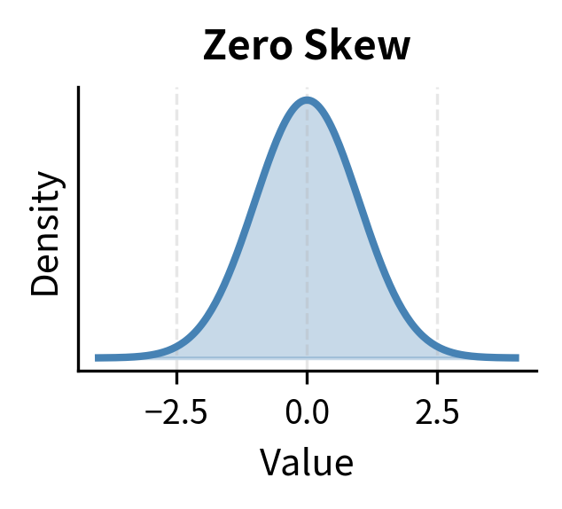
Skewness measures the asymmetry of a distribution. While mean and variance tell us about the center and spread of returns, they assume a symmetric distribution in which gains and losses of equal magnitude are equally likely. Skewness captures deviations from this symmetry, revealing whether the distribution leans toward one side.
The sample skewness is:
where:
- : standardized return (z-score), measuring how many standard deviations each return is from the mean
- The cube preserves the sign, so negative deviations contribute negatively and positive deviations contribute positively
- : number of observations in the sample
- : sample mean return
- : sample standard deviation
Understanding this formula requires recognizing the role of each component. First, we standardize each return by subtracting the mean and dividing by the standard deviation. This creates a dimensionless quantity (the z-score) that measures how unusual each return is in terms of standard deviations. A z-score of 2 means the return was two standard deviations above average.
The key step is raising these standardized returns to the third power. Unlike squaring (which makes everything positive), cubing preserves the sign: negative values remain negative after cubing, while positive values remain positive. Moreover, cubing amplifies extreme values more than moderate ones. A z-score of 3 contributes 27 to the sum, while a z-score of 2 contributes only 8. This means skewness is heavily influenced by the tails of the distribution.particularly by which tail extends further.
The interpretation of skewness values:
- Zero skewness: Symmetric distribution (normal distribution)
- Negative skewness: Left tail is longer; large losses are more likely than large gains
- Positive skewness: Right tail is longer; large gains are more likely than large losses
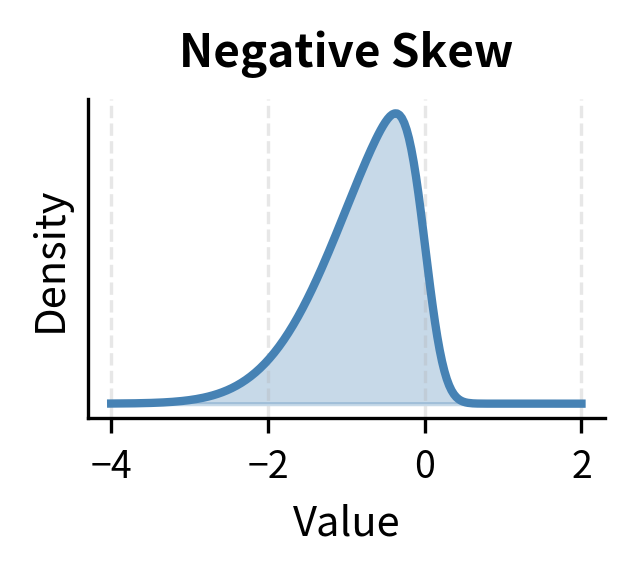
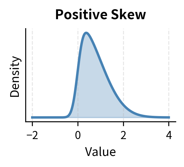
Equity returns typically exhibit negative skewness. Markets tend to fall faster than they rise, creating asymmetric risk. This pattern results from investor behavior: bad news tends to trigger panic selling that drives prices down rapidly, while good news generates more gradual buying. The result is a distribution where extreme negative returns occur more frequently than extreme positive returns of the same magnitude. This matters for risk management: a model assuming symmetry will underestimate the probability of large losses.
The Fourth Moment: Kurtosis
Kurtosis measures the heaviness of the tails relative to a normal distribution. While skewness tells us about asymmetry, kurtosis addresses a different question: how likely are extreme events? A distribution can be perfectly symmetric yet have tails that are much heavier (or lighter) than a normal distribution would predict.
The sample kurtosis is:
where:
- : the fourth power of standardized returns
- The fourth power amplifies extreme values, making kurtosis sensitive to tail observations
- : number of observations
- : sample mean return
- : sample standard deviation
The fourth power creates an even more extreme amplification of outliers than the cube used in skewness. A standardized return of 3 (three standard deviations from the mean) contributes 81 to the sum, while a standardized return of 4 contributes 256. This makes kurtosis very sensitive to tail events. A single extreme observation can dramatically increase the kurtosis estimate, which is both a feature and a limitation: it captures exactly what we want to measure (tail behavior) but with considerable sampling variability.
A normal distribution has a kurtosis of 3. Excess kurtosis subtracts 3 to make the normal distribution the baseline:
where:
- : the raw kurtosis value computed from the sample
- : the kurtosis of the standard normal distribution, used as the reference point (subtracting it makes the normal distribution have excess kurtosis of zero)
By subtracting 3, we create a measure where zero represents "normal" tail behavior. Positive excess kurtosis indicates heavier tails than normal, while negative excess kurtosis indicates lighter tails. Most statistical software, including scipy, reports excess kurtosis by default.
The interpretation of excess kurtosis values:
- Zero: Normal tails (mesokurtic)
- Positive: Heavier tails than normal; extreme events more likely (leptokurtic)
- Negative: Lighter tails than normal; extreme events less likely (platykurtic)
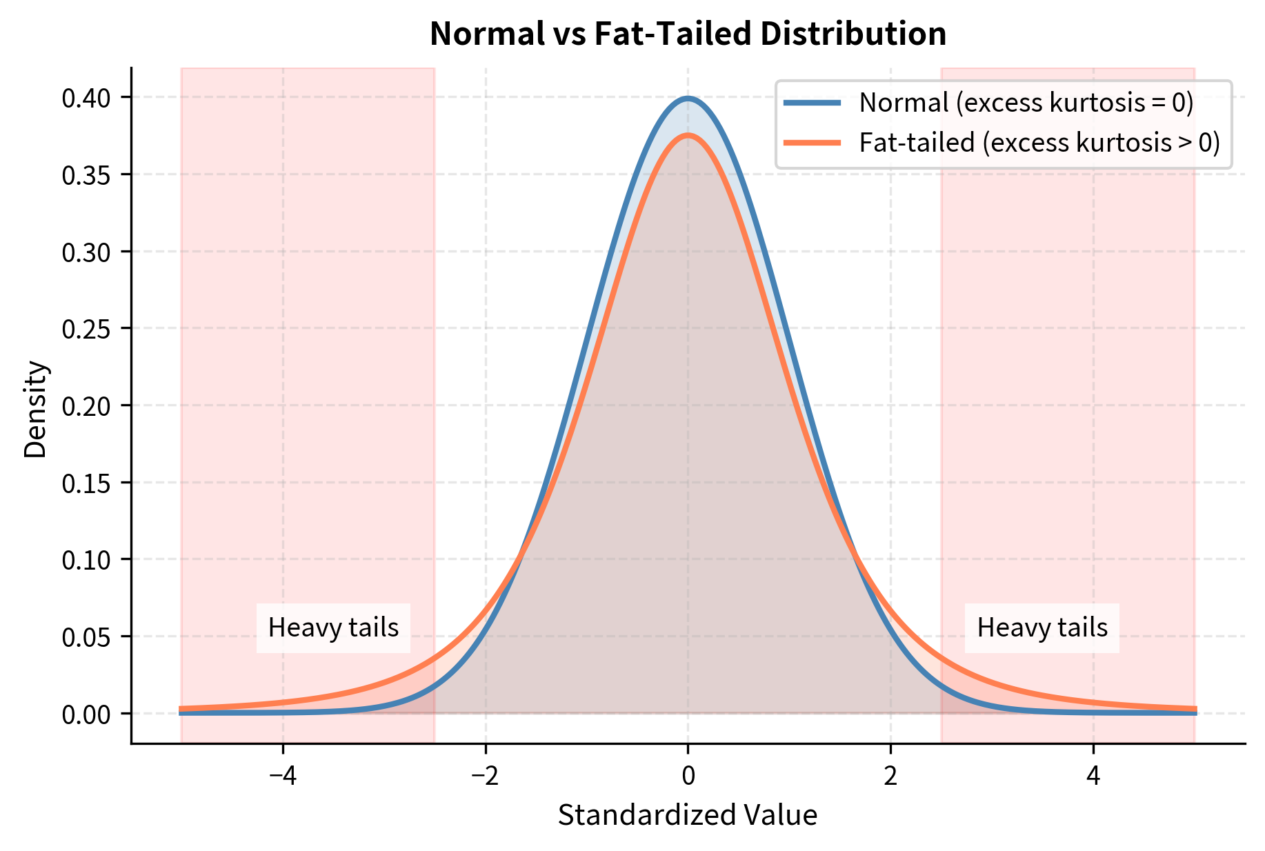
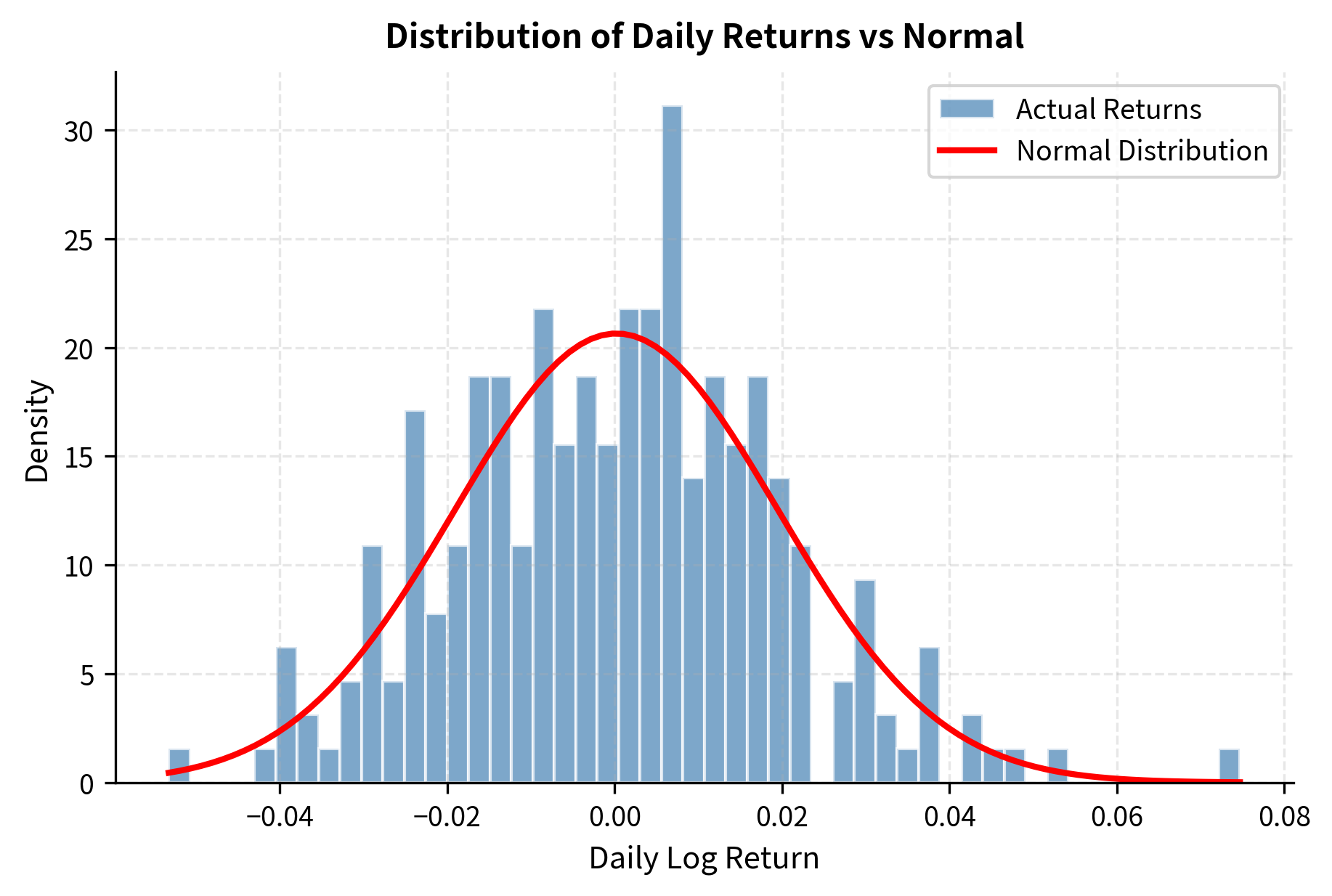
Financial returns almost always exhibit positive excess kurtosis, often called "fat tails," meaning extreme events occur more frequently than a normal distribution predicts. Events that should occur once per century under normal assumptions happen every few years. The 2008 financial crisis, the 2010 flash crash, and the 2020 COVID crash all produced returns that were statistically improbable under a normal distribution. To illustrate, a six-standard-deviation move in one direction should occur roughly once in a billion days under normality, yet financial markets experience such moves with disturbing regularity. This gap between theoretical predictions and observed reality is one of the most important findings in empirical finance.
Visualizing the Distribution
Let's visualize these statistics with a histogram and overlay a normal distribution for comparison:
Summary Statistics Table
Let's create a function that computes all descriptive statistics in one place:
The Sharpe ratio, included above, measures risk-adjusted return by dividing excess return by volatility:
where:
- : annualized mean return of the portfolio or strategy
- : risk-free rate (often assumed to be zero for simplicity, as in the code above)
- : annualized volatility It's one of the most widely used performance metrics in finance.
The Sharpe ratio addresses a fundamental question in investing: how much return are you earning per unit of risk taken? A strategy with high returns might simply be taking excessive risk. The Sharpe ratio normalizes performance by volatility, allowing meaningful comparisons across strategies with different risk profiles. A Sharpe ratio of 1.0 means you earn one percentage point of excess return for each percentage point of volatility.historically, this represents solid performance for a diversified portfolio.
Statistical Inference: From Samples to Populations
Descriptive statistics summarize historical data, but we care about the future. Statistical inference bridges this gap by using sample data to make probabilistic statements about population parameters. This transition from description to inference is perhaps the most important conceptual leap in quantitative analysis.
Sample vs. Population
The distinction between sample and population is fundamental to understanding everything that follows in this section. When we compute a mean return from historical data, we're not calculating the "true" expected return.we're estimating it from limited information.
The population is the complete set of all possible observations. In finance, this might be "all possible daily returns a stock could generate" across an infinite time horizon.
A sample is a subset of observations we actually collect. Historical returns form our sample, typically covering a limited time period.
We observe sample statistics (denoted with bars or hats: , ) and use them to estimate population parameters (denoted with Greek letters: , ). This notational convention serves as a constant reminder that what we calculate from data (sample statistics) and what we're trying to learn about (population parameters) are different quantities.
The key challenge: sample statistics vary from sample to sample. If you calculate the mean return from 2010-2020 versus 2015-2025, you'll get different numbers even for the same stock. This variability is called sampling error. It's not a mistake or a flaw in your analysis; it is an inherent feature of drawing conclusions from incomplete information. Understanding and quantifying this variability is the core task of statistical inference.
The Standard Error
The standard error quantifies how much a sample statistic varies across different samples. It answers: if I collected a new sample of the same size, how different might my estimate be? For the sample mean:
where:
- : standard error of the sample mean, measuring how much would vary across repeated samples
- : population standard deviation (true variability of individual returns)
- : sample size (number of observations)
- The in the denominator reflects that averaging reduces variability, but with diminishing returns.to halve the standard error, you need four times as much data
This formula captures one of the most important relationships in statistics. The standard error depends on two factors: the variability of individual observations () and the sample size (). More variable data produces less precise estimates. Larger samples produce more precise estimates. The square root relationship means precision improves slowly with additional data. This is an example of diminishing returns with significant practical implications.
In practice, we estimate with the sample standard deviation :
This introduces a subtle complication: we're using estimated variability to estimate the precision of another estimate. The sample standard deviation is itself subject to sampling error, which adds uncertainty beyond what the formula suggests. For large samples, this additional uncertainty is negligible, but for small samples, it matters enough that we use the t-distribution rather than the normal distribution for inference.
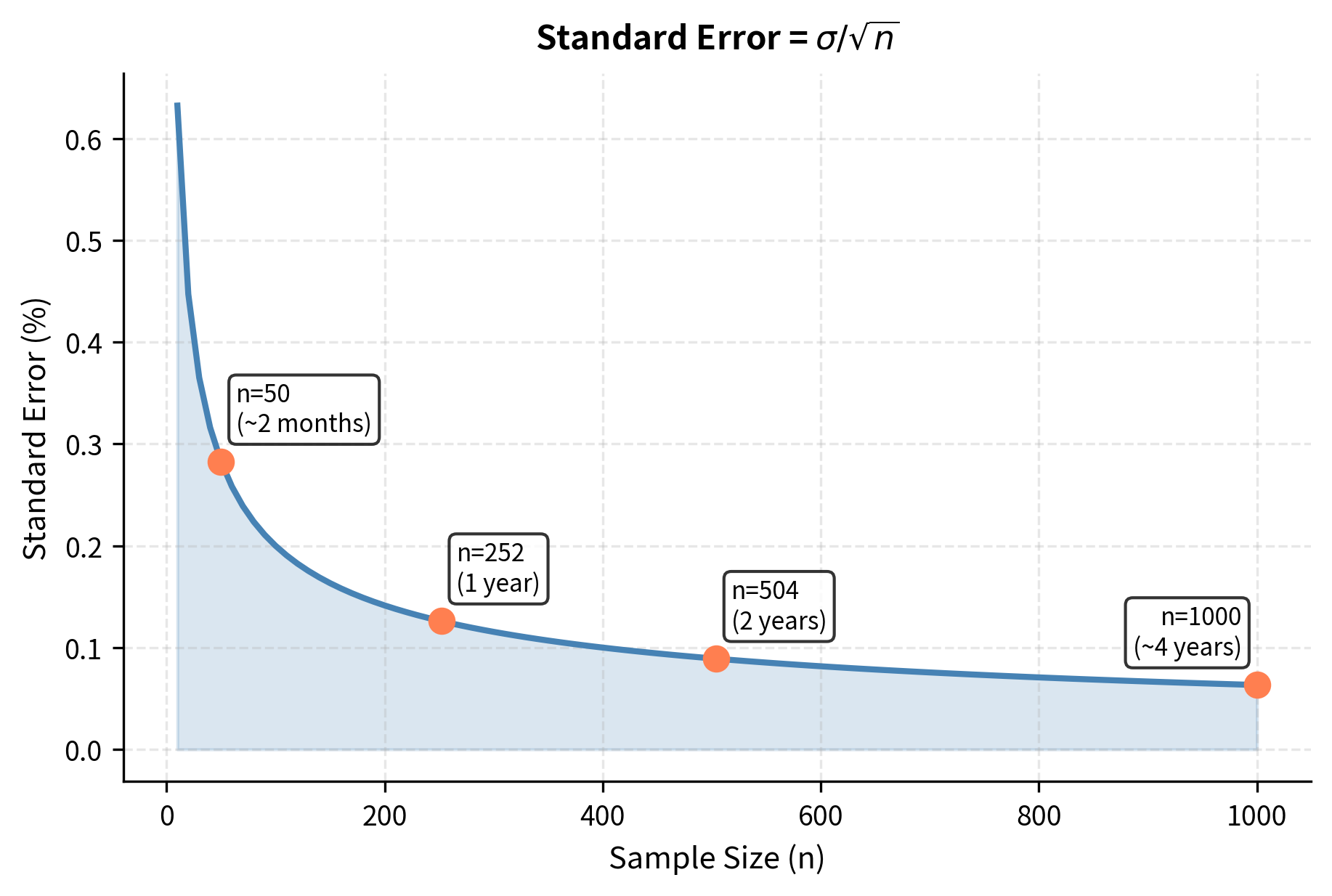
The standard error decreases with the square root of the sample size. To halve your uncertainty, you need four times as much data. This has profound implications for finance. Even with decades of data, mean return estimates remain imprecise. Consider the ratio printed above.the standard error is often comparable in magnitude to the mean itself, indicating that our estimate of expected returns is extremely noisy.
The Central Limit Theorem
The Central Limit Theorem (CLT) is one of the most important results in statistics, and its implications extend beyond textbooks. It provides the theoretical justification for using normal distribution-based methods even when the data themselves are not normally distributed.
If are independent random variables with mean and variance , then as :
where:
- : sample mean
- : population mean
- : standard error of the mean
- : convergence in distribution (meaning the distribution of the left side approaches the distribution on the right as grows)
- : standard normal distribution (mean 0, variance 1)
The left side of the equation is called the standardized sample mean or z-score of the sample mean. The CLT tells us this standardized value becomes approximately normal, regardless of the original distribution's shape.
The sample mean is approximately normally distributed with mean and standard deviation .
This theorem is powerful. It tells us that the distribution of the sample mean converges to a normal distribution regardless of the shape of the underlying distribution. You could be sampling from a distribution that is skewed, fat-tailed, bimodal, or otherwise irregular, yet the mean of a large sample will still be approximately normally distributed.
This result comes from the mathematics of averaging. When you average many independent random variables, the extreme values in both directions tend to cancel out, the moderate values accumulate, and the result is pulled toward the center. This centering effect, repeated across all possible samples, produces the familiar bell curve.
Even if daily returns are not normally distributed (and they're not due to skewness and fat tails), the average of many returns will be approximately normal. This justifies using normal-based inference procedures for sample means.
Let's demonstrate the CLT by repeatedly sampling and computing means:
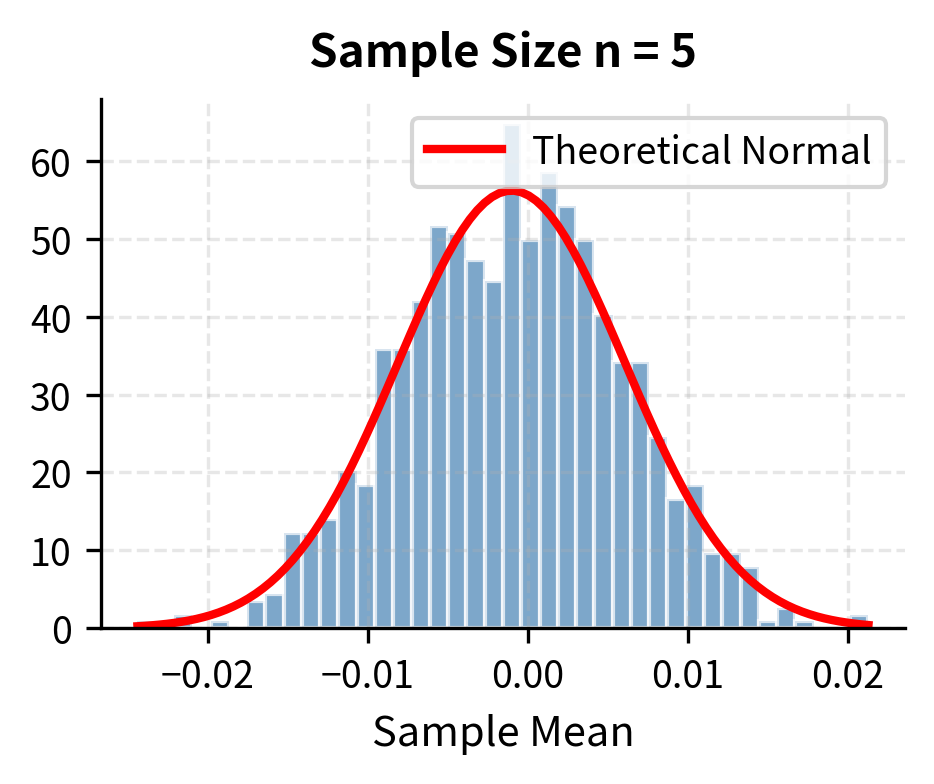
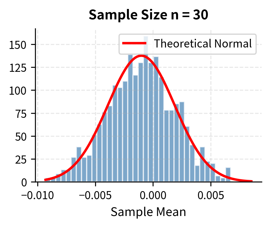
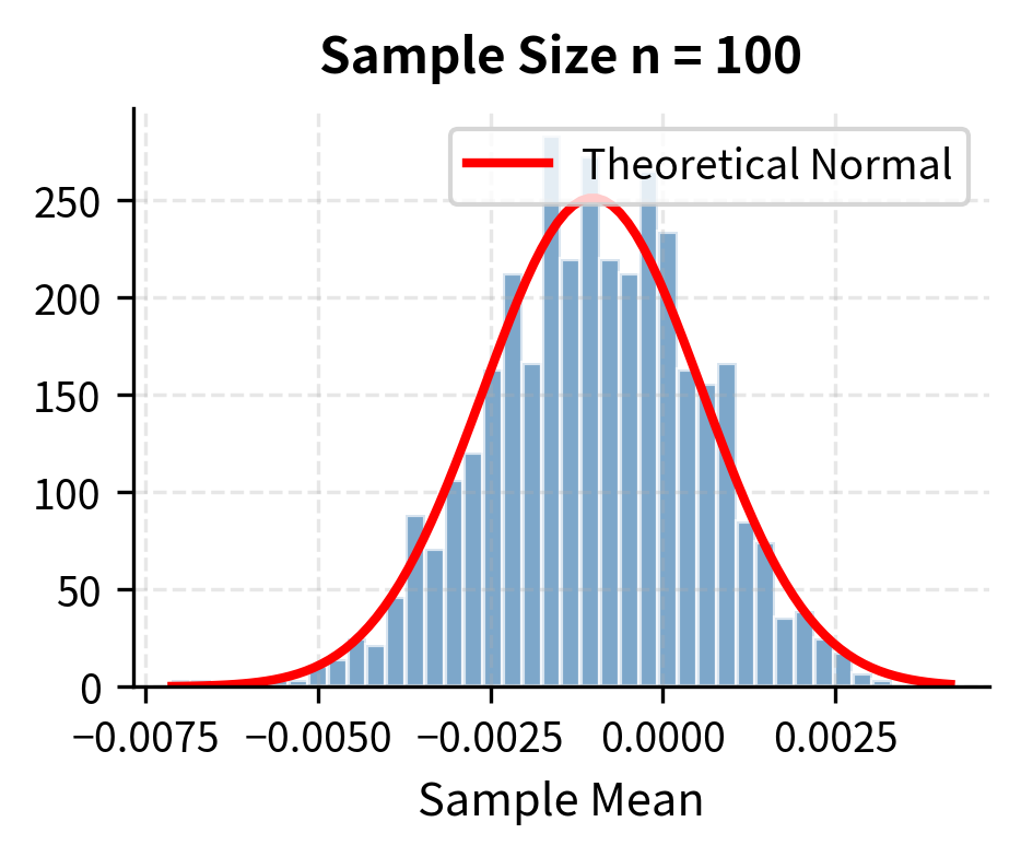
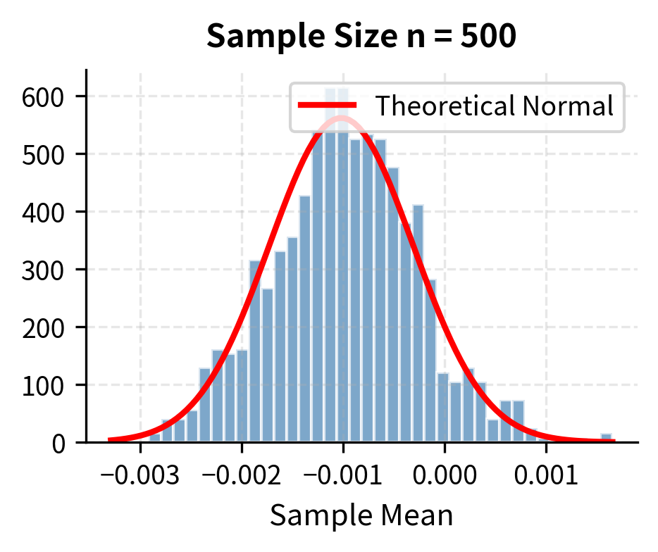
With samples as small as 30, the distribution of sample means is nearly normal, despite the underlying population being clearly non-normal. This is the CLT in action. The figure illustrates the progression: with only 5 observations, the distribution of sample means retains some features of the underlying distribution. By the time we reach 30 observations, the bell-curve shape is evident. With 500 observations, the approximation is essentially perfect.
Hypothesis Testing
Hypothesis testing provides a framework for making decisions based on data. In finance, you might ask: "Is this strategy's return significantly different from zero?" or "Does this factor predict returns?" These questions require a systematic approach that accounts for uncertainty in sample-based estimates.
The Framework
A hypothesis test has four components:
- Null hypothesis (): The default assumption, typically "no effect" or "no difference"
- Alternative hypothesis ( or ): What you're trying to demonstrate
- Test statistic: A number computed from data that measures evidence against
- P-value: The probability of observing a test statistic as extreme as yours if is true
Hypothesis testing works by contradiction. We start by assuming the null hypothesis is true, then ask: given this assumption, how probable is the data we actually observed? If the answer is "very improbable," we reject the null hypothesis. If the answer is "reasonably probable," we fail to reject it. Note the asymmetry: we never "accept" the null hypothesis; we merely fail to find sufficient evidence against it.
The p-value answers the question: "If there were truly no effect, how surprising would my data be?" Small p-values indicate the observed data would be unlikely under the null hypothesis, providing evidence against it. A p-value of 0.01, for example, means there's only a 1% chance of seeing data this extreme if the null hypothesis were true.
If the p-value is below a threshold (commonly ), we reject in favor of . The choice of is a convention, not a law of nature. It represents a balance between two types of errors: rejecting a true null hypothesis (Type I error) and failing to reject a false null hypothesis (Type II error). Lower values of make Type I errors less likely but Type II errors more likely.
Testing if Mean Return Differs from Zero
The most common hypothesis test in strategy evaluation is whether the mean return is significantly different from zero. This test asks whether the observed positive return is likely to reflect genuine skill or strategy edge, or could it simply be the result of random chance?
Under the null hypothesis that the true mean is zero:
The null hypothesis states that the strategy has no edge: its expected return is zero. The alternative hypothesis states that the expected return is not zero (it could be positive or negative). This is a two-tailed test because we're interested in deviations from zero in either direction.
The test statistic is:
where:
- : test statistic
- : sample mean return
- : sample standard deviation (estimate of )
- : estimated standard error
The t-statistic measures how many standard errors the sample mean is from zero. A t-statistic of 2, for example, means the observed mean is 2 standard errors away from the hypothesized value of zero. This would be unusual if the true mean were actually zero. The larger the absolute value of the t-statistic, the stronger the evidence against the null hypothesis.
Under , this follows a t-distribution with degrees of freedom (we lose one degree of freedom because we estimated the mean from the data). The t-distribution is similar to the normal distribution but has heavier tails, reflecting the additional uncertainty from estimating the population standard deviation. As sample size increases, the t-distribution converges to the normal distribution.
One-Tailed vs. Two-Tailed Tests
The test above was two-tailed, asking whether the mean differs from zero in either direction. Often in finance, you care specifically about whether returns are positive:
This formulation changes the question from "is there an effect?" to "is there a positive effect?" The null hypothesis now includes all non-positive values, and we only reject it if we find strong evidence of positive returns.
For a one-tailed test, the p-value is halved (for the appropriate direction) because we only consider extreme values in one tail rather than both:
The Multiple Testing Problem
In practice, quantitative researchers test many strategies, factors, or parameters. If you test 100 strategies at , you expect 5 false positives by chance alone. This is the multiple testing problem, and it represents one of the most significant challenges in quantitative finance research.
The mathematics is straightforward, but its implications are serious. With a 5% false positive rate per test, the probability of at least one false positive across independent tests is . For 100 tests, this exceeds 99%. In other words, finding at least one "significant" result is virtually guaranteed even when no true effects exist.
Bonferroni correction: Divide by the number of tests. Testing 100 strategies? Use .
Benjamini-Hochberg: Controls the false discovery rate (FDR) rather than the family-wise error rate. Less conservative than Bonferroni.
The Bonferroni correction is simple but often too conservative, especially when tests are correlated (as they typically are in finance). The Benjamini-Hochberg procedure offers a different approach by controlling the expected proportion of false discoveries among all discoveries, rather than the probability of any false discovery.
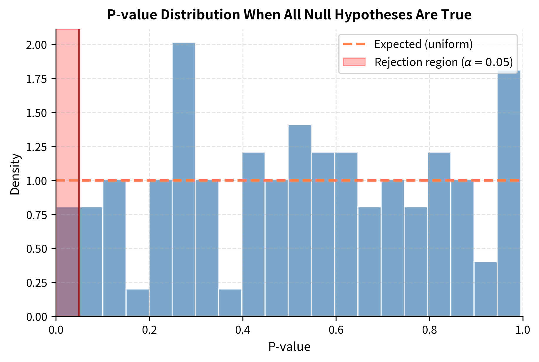
This simulation shows why backtesting results should be viewed skeptically. When you've tested many variations and found one that "works," it may simply be a false positive. The best-performing strategy in a backtest of 100 random strategies will look impressive purely by chance. This phenomenon, sometimes called "p-hacking" or "data dredging," remains common in quantitative finance and requires careful attention.
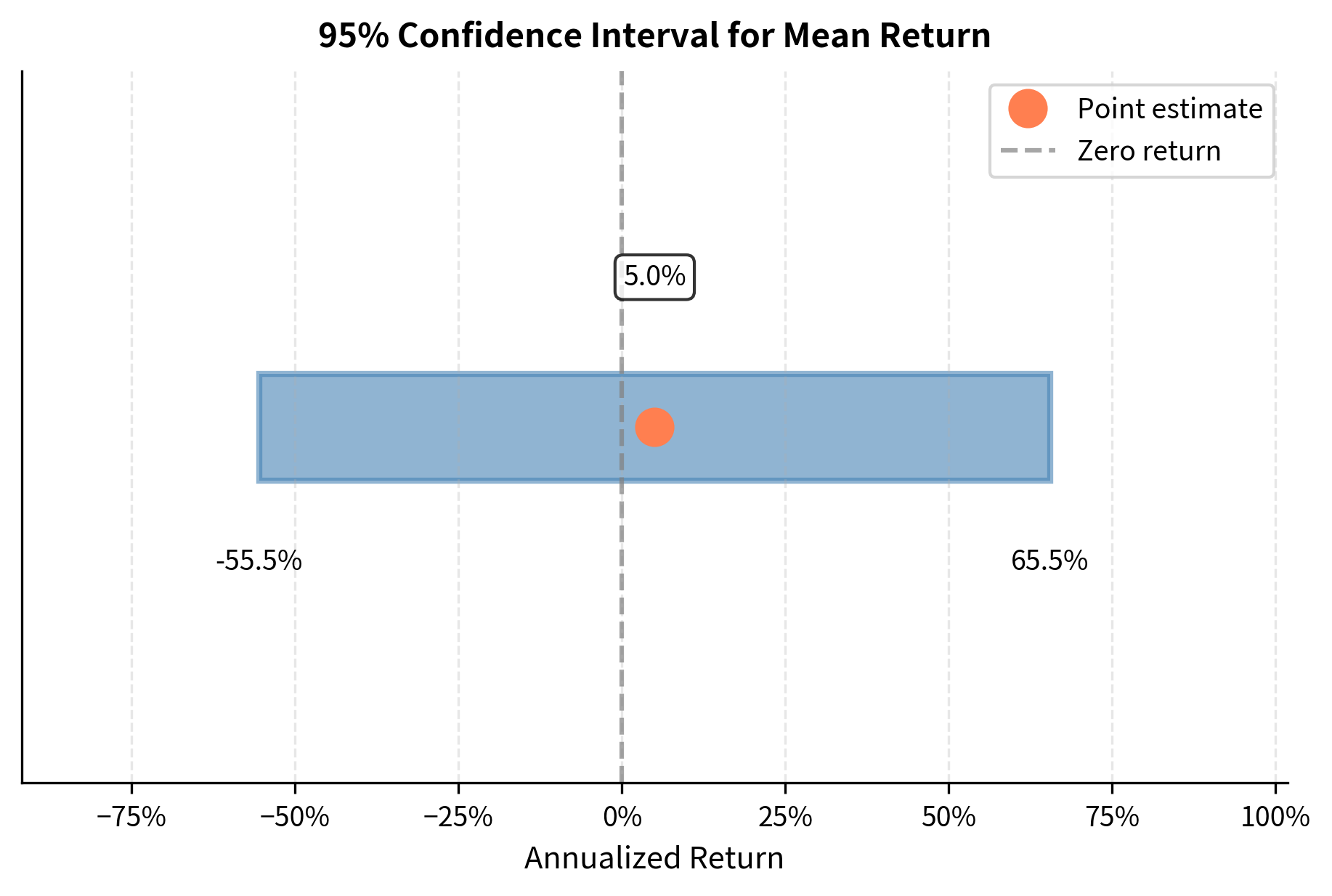
Confidence Intervals
Hypothesis tests give binary decisions, but confidence intervals provide a range of plausible values for a parameter. This additional information is often more useful than a simple yes/no answer because it shows the precision of our estimate.
A 95% confidence interval for the mean return is:
where:
- : sample mean (center of the interval)
- : critical value from the t-distribution with degrees of freedom (the value that cuts off probability in each tail; for 95% confidence with large , this is approximately 1.96)
- : sample size
- : significance level (for 95% confidence, )
- : standard error of the mean
- : margin of error
The construction of this interval follows directly from the sampling distribution of the mean. Approximately 95% of sample means fall within roughly two standard errors of the true mean. Reversing this logic, we can say that an interval extending two standard errors (more precisely, standard errors) in each direction from our observed mean will contain the true mean approximately 95% of the time.
A 95% confidence interval means: if we repeated this sampling procedure many times, 95% of the constructed intervals would contain the true population mean. It does not mean there is a 95% probability the true mean lies in this specific interval. The true mean is fixed; our interval either contains it or it doesn't.
This distinction matters conceptually, even if it rarely changes practical decisions. The frequentist interpretation views probability as a long-run frequency. Across many repetitions of the sampling procedure, 95% of intervals would capture the true parameter. The Bayesian interpretation, which allows probability statements about parameters, requires additional assumptions about prior beliefs.
Confidence Intervals and Risk-Adjusted Returns
Confidence intervals are particularly useful for Sharpe ratios, which are notoriously imprecise. A strategy might show a Sharpe ratio of 1.0, but the confidence interval could span from 0.2 to 1.8, which would change our assessment of the strategy's quality.
Worked Example: Analyzing Real Strategy Returns
Let's walk through a complete statistical analysis of a hypothetical trading strategy. We'll generate returns that mimic a momentum strategy with realistic characteristics.
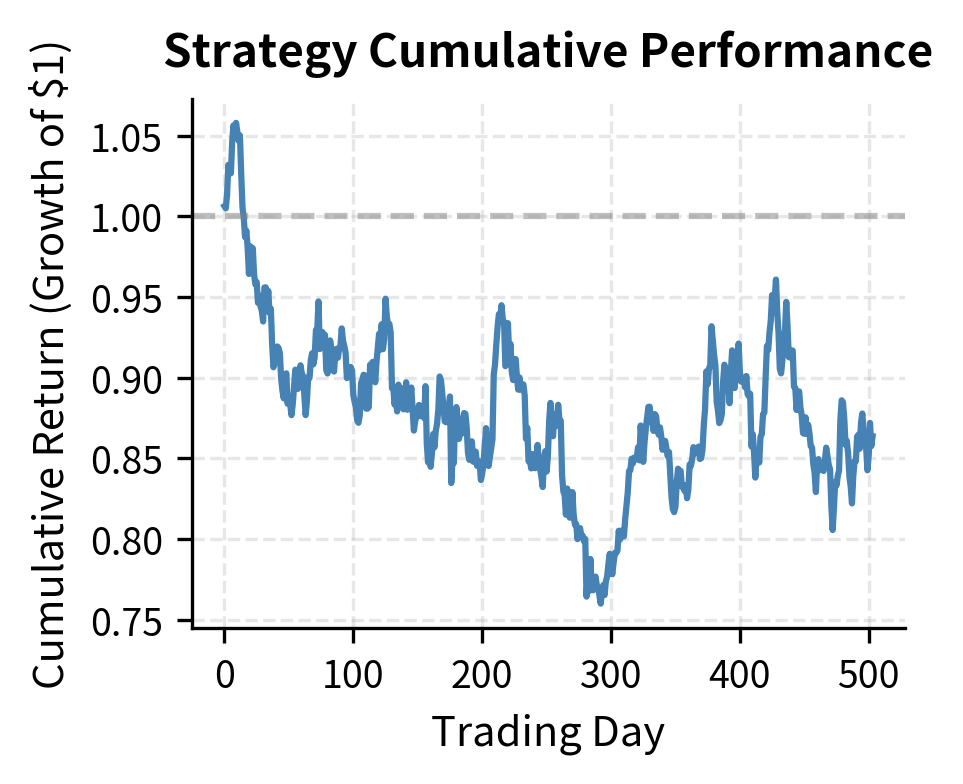
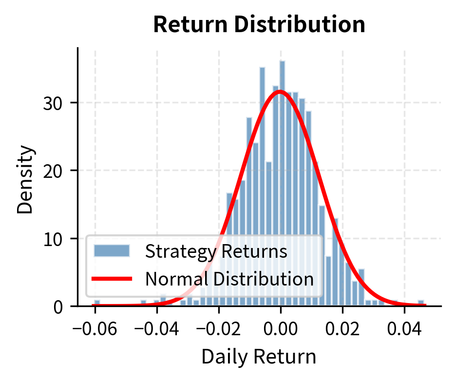
The negative skewness and high kurtosis are characteristic of momentum strategies, which tend to have many small gains punctuated by occasional sharp losses during "momentum crashes."
Key Parameters
The key parameters for statistical analysis of returns:
- n: Sample size (number of observations). Larger samples reduce standard errors and narrow confidence intervals, improving estimation precision.
- α (alpha): Significance level for hypothesis tests (commonly 0.05). Lower values reduce false positive rates but increase false negatives.
- ddof: Degrees of freedom adjustment for variance estimation. Use ddof=1 for sample statistics to get unbiased estimates.
- periods_per_year: Annualization factor (252 for daily trading data). Scales daily statistics to annual equivalents.
- confidence_level: Probability coverage for confidence intervals (commonly 0.95). Higher levels produce wider intervals.
Limitations and Practical Considerations
Statistical inference in finance faces several challenges that don't arise in controlled experiments.
The biggest issue is non-stationarity. Financial markets evolve over time. The distribution of returns in 2020 differs from that in 2010, which in turn differs from 2000. When you estimate a mean from historical data, you are implicitly assuming that past returns are informative about future returns. This assumption is weak at best. Regime changes, structural breaks, and evolving market microstructure all violate the identical distribution assumption underlying classical statistics.
A second challenge is the low signal-to-noise ratio in financial data. Daily returns have a standard deviation roughly 10-20 times larger than their mean. Extracting reliable estimates of expected returns requires large samples. Consider that even with 20 years of daily data (about 5,000 observations), the 95% confidence interval for annualized mean return spans several percentage points. Markets simply do not provide enough data to estimate expected returns precisely.
Serial correlation and clustering of volatility further complicate matters. Returns today are correlated with returns yesterday, though weakly, and volatility exhibits strong persistence. Standard errors computed under independence assumptions understate the true uncertainty. Heteroskedasticity, meaning time-varying volatility, is the norm rather than the exception.
These limitations do not render statistical analysis useless. Instead, they require humility. Treat point estimates with skepticism. Prefer wide confidence intervals to false precision. Consider robust statistics that are less sensitive to outliers. And always remember that statistical significance is not the same as economic significance or practical tradability.
Summary
This chapter covered the statistical foundation for analyzing financial data. We covered the key concepts that you'll use throughout quantitative finance.
Descriptive statistics capture the essential features of return distributions. The mean measures expected return, while volatility quantifies risk. Skewness reveals asymmetry (financial returns are typically left-skewed), and kurtosis captures tail thickness (financial returns have fat tails). Together, these four moments provide a comprehensive summary of return characteristics.
Statistical inference bridges the gap between historical samples and future predictions. The standard error quantifies uncertainty in estimates, with precision improving as the square root of sample size. The Central Limit Theorem justifies normal-based inference for sample means, even when individual returns are non-normal.
Hypothesis testing provides a framework for decision-making under uncertainty. This chapter demonstrated how to test whether a strategy's returns differ from zero using t-statistics and p-values. The multiple testing problem warns against data mining: testing many hypotheses inflates false positive rates.
Confidence intervals offer more information than binary hypothesis tests. For instance, a 95% confidence interval for the Sharpe ratio shows the range of plausible values given your data. Wide intervals signal imprecision and should temper confidence in conclusions.
These tools form the basis for portfolio construction, risk management, and strategy evaluation. As you progress to more advanced topics, you'll encounter sophisticated extensions of these basic ideas. The principles of estimation, uncertainty quantification, and statistical inference remain the same.
Quiz
Ready to test your understanding? Take this quick quiz to reinforce what you've learned about statistical data analysis and inference in finance.

Comments