

Learn bond pricing through present value calculations, yield to maturity analysis, and price-yield relationships. Master fixed income fundamentals.
Choose your expertise level to adjust how many terms are explained. Beginners see more tooltips, experts see fewer to maintain reading flow. Hover over underlined terms for instant definitions.
Bond Fundamentals and Pricing
Bonds are among the oldest and most widely held financial instruments in global markets. When a government needs to fund infrastructure or a corporation wants to expand its operations, issuing bonds allows them to borrow money from investors with a promise to pay it back with interest. Unlike equity, which represents ownership in a company, a bond represents a loan, and the bondholder is a creditor, not an owner.
Understanding bonds is essential for quantitative finance because they form the foundation of fixed income markets, which are much larger than equity markets by total size. The global bond market exceeds $130 trillion in outstanding debt, encompassing government securities, corporate bonds, mortgage-backed securities, and municipal debt. Bond pricing concepts also underpin derivatives valuation, risk management, and portfolio construction.
This chapter introduces the fundamental characteristics of bonds, develops the mathematical framework for pricing them through present value calculations, and explores the conventions and nuances that practitioners encounter daily.
Anatomy of a Bond
A bond is a contractual agreement between an issuer (the borrower) and investors (the lenders). The issuer promises to make a series of payments according to a predetermined schedule in exchange for receiving capital upfront. The key parameters that define a bond are:
-
Face Value (Par Value): The principal amount the issuer promises to repay at maturity, typically $1,000 for corporate bonds or $100 for government bonds in pricing conventions. This is the baseline for calculating coupon payments.
-
Coupon Rate: The annual interest rate applied to the face value to determine periodic payments. A 5% coupon on a $1,000 face value bond pays $50 per year in interest.
-
Maturity Date: The date when the issuer must repay the face value. Maturities range from short-term (under 1 year) to long-term (30 years or more).
-
Payment Frequency: How often coupon payments occur. Most bonds pay semiannually in the US, while European bonds often pay annually.
-
Issuer: The entity borrowing money. Issuers include sovereign governments, municipalities, corporations, and supranational organizations.
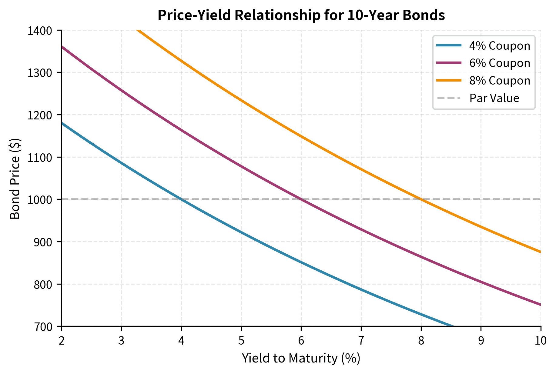
A bond trades at par when its price equals its face value, at a premium when the price exceeds face value, and at a discount when the price is below face value. These relationships depend on how the bond's coupon rate compares to prevailing market interest rates.
Government vs. Corporate Bonds
Government bonds issued by stable sovereigns like US Treasuries or German Bunds are considered nearly risk-free because these governments can tax citizens or, in some cases, print currency to meet obligations. The yields on these bonds serve as benchmarks for pricing all other fixed income securities.
Corporate bonds carry credit risk because companies can default on their obligations. To compensate investors for this risk, corporate bonds offer higher yields than comparable government securities. The difference between a corporate bond's yield and the risk-free rate is called the credit spread, which reflects the market's assessment of default probability and recovery rates.
Cash Flow Patterns
The cash flows from a bond follow predictable patterns determined by its structure. Understanding these patterns is the first step toward pricing bonds accurately. Before assigning a dollar value to any financial instrument, we need to identify exactly what it promises to deliver and when. For bonds, this mapping is transparent. The issuer commits to a specific schedule of payments at the moment of issuance, and these obligations are legally binding. This predictability is what distinguishes fixed income from equity, where future dividends depend on uncertain corporate performance.
Coupon Bonds
A standard coupon bond generates two types of cash flows: periodic coupon payments during its life and a final principal repayment at maturity. For a bond with face value , annual coupon rate , and semiannual payments, each coupon payment equals .
The logic behind this calculation is straightforward. If a bond promises 6% annual interest on a $1,000 face value, the total annual interest obligation is $60. When this interest is distributed across two semiannual payments, each payment becomes $30. This division of the annual coupon into smaller periodic payments has important implications for how we measure yield and compare bonds, as we will see when discussing compounding conventions.
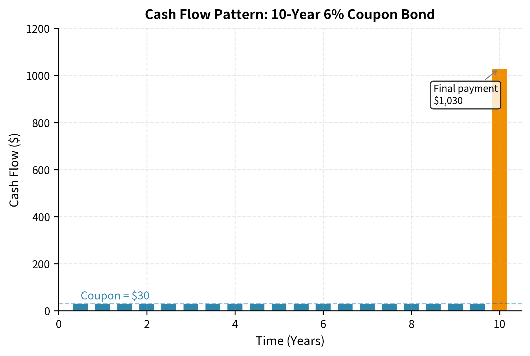
Consider a 10-year bond with a $1,000 face value and 6% annual coupon paid semiannually. The bondholder receives:
- 20 coupon payments of $30 each (every 6 months for 10 years)
- One principal payment of $1,000 at maturity
The final payment at maturity includes both the last coupon and the face value, totaling $1,030.
The total undiscounted cash flows exceed the face value by the cumulative interest payments. However, money received in the future is worth less than money today, which brings us to bond pricing.
Zero-Coupon Bonds
Zero-coupon bonds pay no periodic interest. They are sold at a discount to face value and pay the full face value at maturity. The investor's return comes entirely from price appreciation.
US Treasury bills (T-bills) with maturities up to one year are zero-coupon instruments. A T-bill with a face value of $10,000 might sell for $9,800, with the $200 difference representing the investor's interest income.
Zero-coupon bonds are conceptually simpler because they involve only a single cash flow. This makes them useful building blocks for understanding more complex instruments. Any coupon bond can be decomposed into a portfolio of zero-coupon bonds, one for each cash flow date. This decomposition, known as "stripping" a bond, shows that a coupon bond is a bundle of zero-coupon bonds packaged together. The US Treasury even facilitates this decomposition through its STRIPS program (Separate Trading of Registered Interest and Principal of Securities), which allows investors to trade individual cash flows from Treasury bonds as standalone securities.
Bond Pricing by Discounting Cash Flows
The price of a bond equals the present value of all its future cash flows, discounted at an appropriate rate. This principle connects bond valuation to the time value of money. Bond pricing answers this simple question. What would a rational investor pay today in exchange for a known stream of future payments? The answer requires us to account for the opportunity cost of capital, the return an investor could earn by deploying funds elsewhere.
Present Value Framework
The concept of present value rests on a foundational principle of finance: a dollar today is worth more than a dollar tomorrow. This isn't merely about inflation or risk. It reflects the ability to invest money and earn a return. If you have $100 today and can invest it at 5% for one year, you'll have $105 next year. Working backward, $105 received one year from now is equivalent to having $100 today. Its present value is $100. This backward calculation, called discounting, underlies all bond pricing.
For a bond with cash flows occurring at times years from now, the price is:
where:
- : current price of the bond
- : cash flow received at time (coupon or principal)
- : time in years until the -th cash flow
- : annual discount rate (yield)
- : total number of cash flows
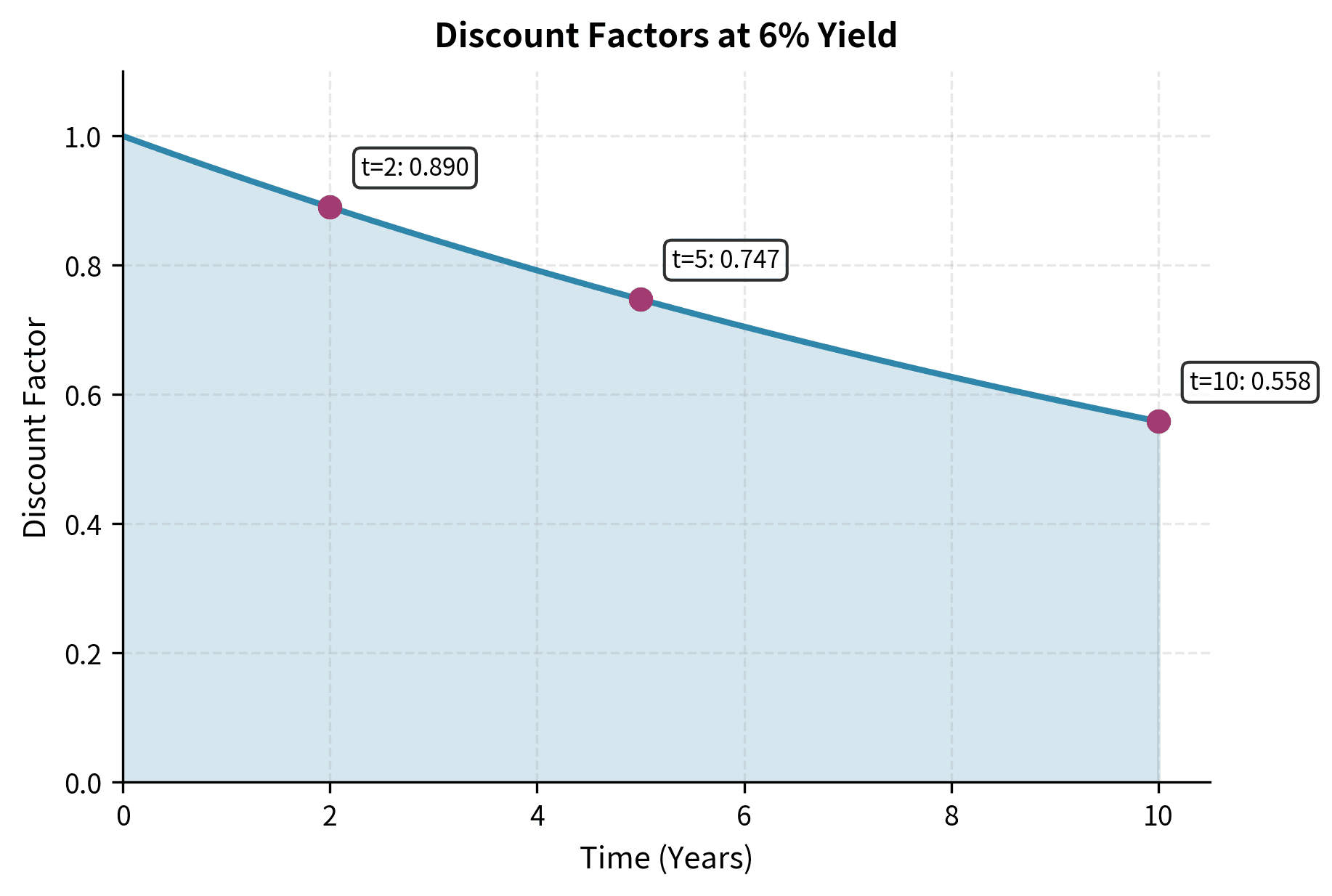
This formula shows that each future cash flow must be discounted back to today's dollars. The denominator represents the growth factor, how much a dollar invested today would become by time . Dividing by this factor reverses the growth, telling us what future dollars are worth in today's terms. The further away a cash flow, the more heavily it is discounted, reflecting the time value of money. A payment arriving in ten years must be divided by a much larger growth factor than one arriving in six months because money has more time to compound.
When payments occur more frequently than annually, we must adjust for compounding. The compounding frequency matters because interest earned on earlier payments can itself earn interest. With payments per year and a yield , the price becomes:
where:
- : bond price
- : cash flow at period
- : annual yield to maturity
- : number of payment periods per year
- : total number of payment periods
- : period counter (1, 2, ..., )
Here, counts payment periods rather than years, and we divide the annual yield by to get the per-period rate. This adjustment accounts for the compounding frequency. A bond paying semiannually compounds twice per year, so we use half the annual rate for each six-month period. The distinction matters. A 6% annual yield compounded semiannually is not the same as a 6% yield compounded annually. With semiannual compounding, you earn 3% in the first half of the year, then 3% on that larger balance in the second half, resulting in an effective annual yield slightly above 6%.
Pricing a Coupon Bond
Now that we understand how to discount individual cash flows, we can develop a simpler formula for pricing standard coupon bonds. Rather than discounting each payment individually, we can exploit the regular structure of coupon payments to derive a closed-form expression that separates the bond's value into two intuitive components.
For a standard coupon bond, we can separate the cash flows into an annuity (the coupons) and a lump sum (the face value). The coupon payments form what mathematicians call an ordinary annuity, a sequence of equal payments occurring at regular intervals. A compact formula exists for the present value of such an annuity, which we can combine with the discounted principal to get the total bond price.
Let be the coupon rate, the face value, the yield, the payment frequency, and the total number of periods. The price is:
where:
- : bond price
- : annual coupon rate (as a decimal)
- : face value (par value)
- : number of coupon payments per year
- : annual yield to maturity
- : total number of coupon periods ()
- : the periodic coupon payment amount
- : the present value annuity factor
The formula separates bond value into two components:
-
Coupon annuity (first term): The stream of periodic coupon payments forms an ordinary annuity. The annuity factor represents how much a dollar paid each period for periods is worth today. It's the sum of all the individual discount factors. To understand this factor, imagine receiving $1 at the end of each period for periods. The present value of the first dollar is , the second is , and so on. The annuity factor is simply the sum of this geometric series, expressed in a single formula. As the number of periods increases or the yield decreases, this factor grows. You're receiving more dollars, or each dollar is worth more in present value terms.
-
Principal repayment (second term): The face value received at maturity, discounted back to today by the factor . This term captures the return of the investor's principal. For long-maturity bonds, this discount factor can be quite small. At a 6% yield compounded semiannually over 30 years, the discount factor is approximately 0.17, meaning the present value of the $1,000 face value is only about $170.
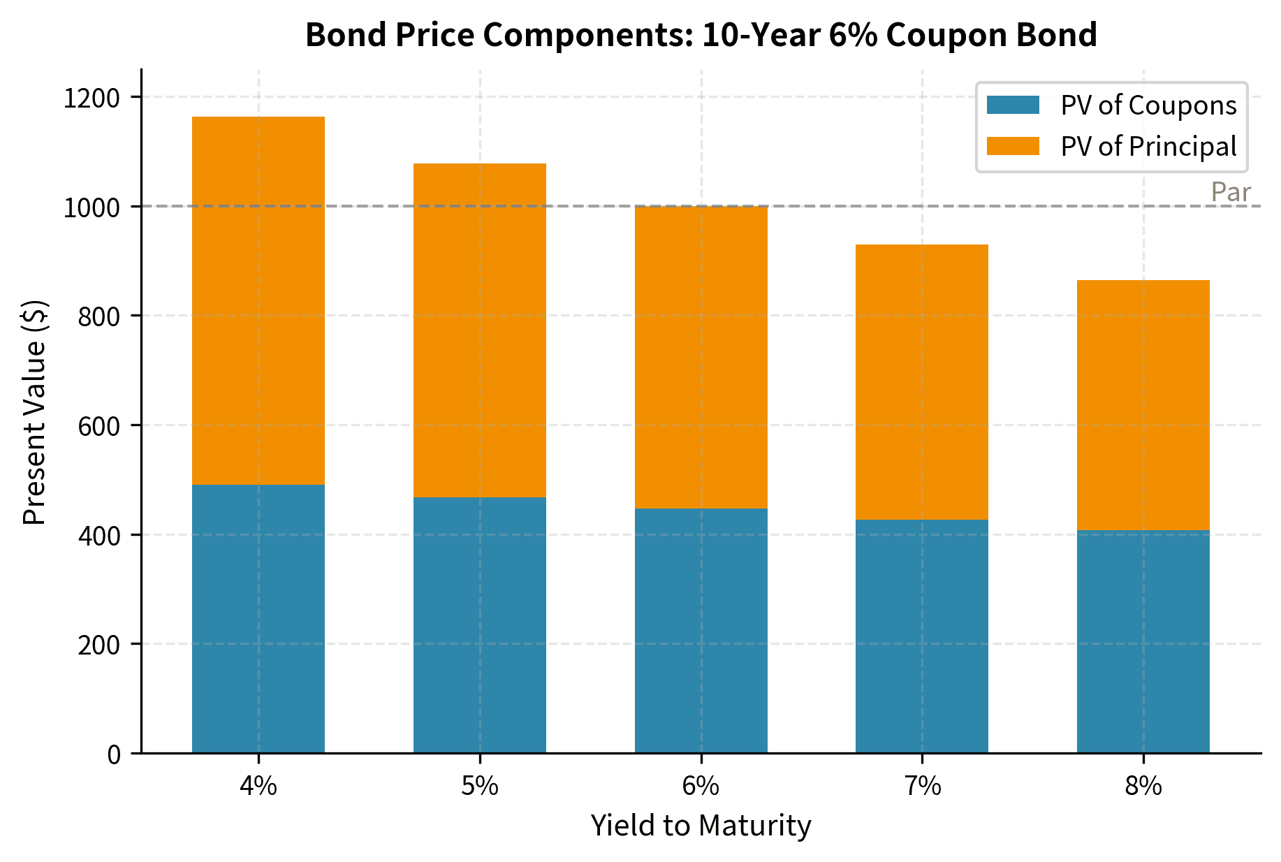
This decomposition reveals why bond prices respond to yield changes: when yields rise, both discount factors shrink, reducing the present value of all future cash flows. The principal's contribution to price sensitivity increases for lower-coupon bonds because a larger fraction of total value comes from the distant lump-sum payment rather than the near-term coupon stream. A zero-coupon bond is the extreme case where 100% of the value comes from the principal payment, making it most sensitive to yield changes.
This demonstrates the inverse relationship between yields and prices. When the yield equals the coupon rate (6%), the bond trades at par. When yields fall below the coupon rate, the bond trades at a premium because its fixed coupons are more attractive than market rates. When yields rise above the coupon rate, the bond trades at a discount.
The economic intuition behind premium and discount bonds is worth exploring. Consider a world where newly issued bonds offer 7% coupons. An existing 6% coupon bond becomes less attractive by comparison. Why accept $60 per year when you could buy a new bond paying $70? The only way the old bond can compete is by offering a lower price, allowing the buyer to capture additional return through price appreciation to par at maturity. This price adjustment mechanism ensures that all bonds of similar risk and maturity offer comparable total returns, regardless of their stated coupon rates.
Pricing a Zero-Coupon Bond
Zero-coupon bonds strip away the complexity of multiple cash flows, leaving us with the purest expression of present value. With only a single payment at maturity, the pricing formula reduces to its most elemental form, making zero-coupon bonds ideal pedagogical tools for understanding how time and yield interact to determine value.
Zero-coupon bonds have a simpler pricing formula since there's only one cash flow:
where:
- : current price of the zero-coupon bond
- : face value paid at maturity
- : annual yield (discount rate)
- : time to maturity in years
The simplicity of this formula makes zero-coupon bonds ideal building blocks for understanding fixed income. The price represents exactly how much an investor must pay today to receive dollars in years, given the market's required return of . Notice that the price is always less than the face value (assuming a positive yield), and the discount increases with both yield and time to maturity. A 30-year zero-coupon bond at a 5% yield trades at roughly 23% of its face value, reflecting the substantial time value of money over such a long horizon.
The zero-coupon bond's price sensitivity to yield changes is more pronounced because all the value comes from a single distant cash flow. With no intervening coupons to provide partial early recovery of the investment, the entire value of a zero-coupon bond is subject to the full discounting effect over the entire time to maturity.
Yield to Maturity
While we've been using yield as an input to calculate price, in practice traders observe market prices and need to calculate the implied yield. The yield to maturity (YTM) is the single discount rate that equates a bond's price to the present value of its cash flows. In essence, YTM answers the question: what constant annual return is embedded in today's market price?
The yield to maturity is the internal rate of return (IRR) of a bond investment, assuming the investor holds the bond until maturity and reinvests all coupon payments at the same yield. It provides a standardized measure for comparing bonds with different coupons and maturities.
Calculating YTM
The calculation of yield to maturity reverses the pricing problem we solved earlier. Instead of taking a yield and computing a price, we observe a market price and work backward to find the yield that makes our pricing formula produce that exact price. This inversion transforms what was a straightforward arithmetic problem into one that requires iteration to solve.
Finding the YTM requires solving for in the bond pricing equation:
where:
- : observed market price (known)
- : yield to maturity (unknown, to be solved)
- , , : as defined previously
This equation has no closed-form solution for coupon bonds because appears in the denominator of multiple terms with different exponents. The mathematical challenge arises because we cannot isolate algebraically. It is buried inside discount factors raised to various powers, and these terms are summed together. We must use numerical methods such as Newton-Raphson iteration or Brent's root-finding algorithm to find the that makes the equation hold. These algorithms work by making intelligent guesses and progressively refining them until the calculated price matches the market price to within an acceptable tolerance.
The results confirm our earlier observation: premium bonds (price > par) have yields below the coupon rate, while discount bonds have yields above the coupon rate.
YTM Assumptions and Limitations
The YTM calculation makes two important assumptions that rarely hold in practice:
-
Hold to maturity: It assumes the investor holds the bond until maturity. If the investor sells before maturity, the realized return depends on the prevailing market price, which may differ from the purchase price.
-
Constant reinvestment rate: It assumes all coupon payments can be reinvested at the same YTM. In reality, interest rates fluctuate, so reinvestment occurs at varying rates. This reinvestment risk means the actual return may differ from the YTM, particularly for long-maturity bonds with high coupons. Consider a 30-year bond with a 10% coupon. Over three decades, the investor will receive 60 coupon payments, each of which must be reinvested. The assumption that all these reinvestments occur at exactly 10% is unrealistic. Interest rates will inevitably vary over such a long period.
Despite these limitations, YTM remains the standard measure for comparing bond investments. It captures the total return from coupons, reinvestment, and price changes to maturity.
Fixed Rate vs. Floating Rate Bonds
The bonds we've discussed so far have fixed coupon rates set at issuance. Floating rate bonds (or floating rate notes, FRNs) have coupon rates that reset periodically based on a reference rate plus a spread. This fundamental structural difference creates very different risk profiles and pricing dynamics.
Floating Rate Mechanics
A typical floating rate bond might pay 3-month SOFR (Secured Overnight Financing Rate) plus 100 basis points, resetting quarterly. If SOFR is 4.5% at a reset date, the coupon for the next quarter would be 5.5% annualized.
The coupon for each period is calculated as:
where:
- : the interest rate for the upcoming coupon period
- : the benchmark rate observed at reset (e.g., SOFR, previously LIBOR)
- : the fixed margin over the reference rate, set at issuance to reflect credit risk
The reference rate is typically observed at the beginning of each coupon period (or with a short lookback), and the spread is fixed at issuance to reflect the issuer's credit quality. This structure transfers interest rate risk from the investor to the issuer. If market rates rise, the issuer pays higher coupons. If rates fall, the issuer pays lower coupons. For investors seeking to minimize interest rate exposure while maintaining credit exposure, floating rate notes work well.
Pricing Floating Rate Bonds
The pricing of floating rate bonds follows a fundamentally different logic than fixed rate bonds. Because future coupons are unknown (since they depend on future reference rate realizations), we cannot simply discount a known cash flow stream. Instead, we rely on a key insight: at each reset date, the bond's coupon adjusts to match market rates, so the bond should trade at par.
At each reset date, a floating rate bond trading at par should continue to trade at par (assuming no change in credit quality) because its coupon adjusts to market rates. Between reset dates, the price may deviate slightly from par due to the fixed coupon rate for the current period.
The price immediately after a reset date is approximately:
where:
- : current price of the floating rate note
- : face value
- : current coupon rate (fixed for this period)
- : current reference rate (e.g., SOFR)
- : time in years until the next coupon reset
- : the "excess" or "deficit" interest for the current period
The intuition is straightforward. If the current coupon exceeds the market rate , the bond is worth slightly more than par because the holder receives above-market interest until the next reset. Conversely, if , the bond trades below par. At the reset date (), the price equals exactly . The deviation from par represents the present value of the coupon differential, the difference between what the bond actually pays and what a newly issued bond would pay, accumulated over the remaining time until the next reset.
The floating rate note trades at 1.22 above par. This small premium reflects the fact that the current coupon rate (5.5%) slightly exceeds what the market would set today given the reference rate plus spread. The minimal deviation from par illustrates why floating rate bonds have much lower interest rate risk than fixed rate bonds. Their prices remain stable as market rates change because future coupons adjust accordingly. This stability makes floating rate notes attractive to investors who want credit exposure without taking on substantial interest rate risk.
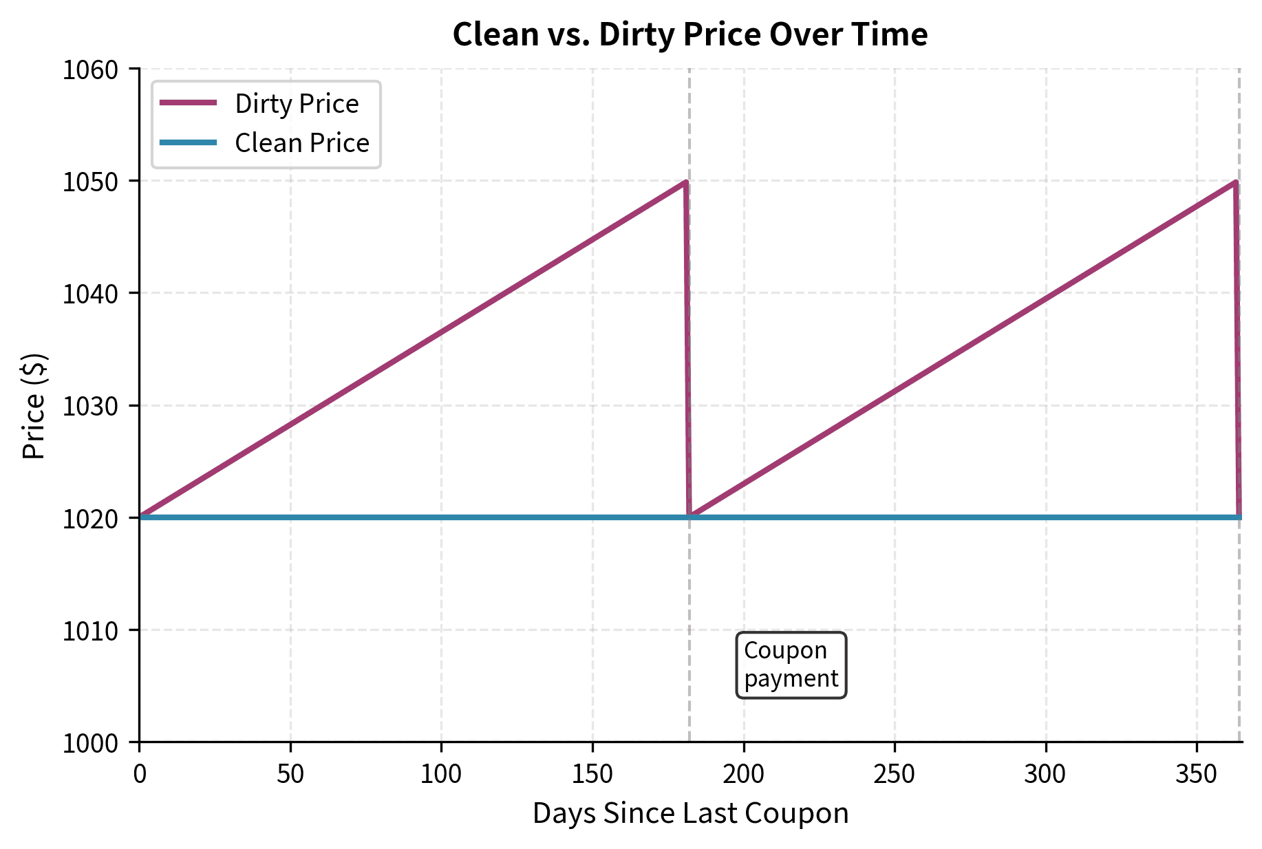
Clean Price, Dirty Price, and Accrued Interest
Bond prices in the market are quoted as clean prices, but the actual amount paid in a transaction is the dirty price (also called the full price or invoice price). The difference is accrued interest. This distinction matters for anyone trading bonds, as confusing clean and dirty prices can lead to costly errors.
Understanding Accrued Interest
When you buy a bond between coupon dates, you must compensate the seller for the interest that has accumulated since the last coupon payment. The seller held the bond during part of the coupon period and is entitled to that portion of the upcoming coupon. This ensures that the seller receives fair value for the time they held the bond, while the buyer is not penalized for purchasing mid-period.
To understand why accrued interest exists, consider what happens when the next coupon is paid. The issuer sends the full coupon to whoever holds the bond on the payment date. There's no mechanism to split the payment between the old and new owners. Therefore, the buyer, who will receive the full coupon, must reimburse the seller for the portion of interest that accrued while the seller held the bond. This is the accrued interest.
Accrued interest is calculated as:
where:
- : the full periodic coupon amount (e.g., )
- : calendar days from the last payment date to settlement
- : total days in the current coupon period
The fraction represents the portion of the coupon period that has elapsed. This is the seller's "fair share" of the upcoming coupon. If exactly half the period has elapsed, the seller is entitled to half the coupon.
The dirty price is then:
where:
- : the actual cash amount paid in the transaction
- : the quoted market price (excludes accrued interest)
Markets quote clean prices because dirty prices jump discontinuously at coupon payment dates. The clean price provides a smoother series that better reflects changes in interest rates and credit conditions rather than the mechanical passage of time through a coupon period.
When the buyer receives the next coupon payment, it will compensate them for both the accrued interest they paid and the interest earned during the remaining portion of the period they held the bond.
Day Count Conventions
The calculation of accrued interest depends on how days are counted, which varies by market and instrument type. These day count conventions affect both the numerator (days elapsed) and denominator (days in the period or year) of interest calculations. Though this seems like a minor technicality, day count conventions can significantly affect payments and valuations, particularly for large positions or over extended periods.
Common Conventions
The diversity of day count conventions reflects the historical evolution of different markets and the practical tradeoffs between computational simplicity and mathematical precision. Before computers were common, simpler conventions like 30/360 reduced calculation effort, while actual day counts provide more accurate accruals.
The most widely used day count conventions are:
-
Actual/Actual (Act/Act): Uses the actual number of days in the numerator and the actual number of days in the coupon period for the denominator. This is standard for US Treasury bonds and many government securities. It's the most precise convention but requires knowing the specific dates of each coupon period.
-
30/360: Assumes each month has 30 days and each year has 360 days. This simplifies calculations and is common for US corporate and municipal bonds. Under this convention, February is treated as having 30 days, and all months contribute equally to interest accrual.
-
Actual/360: Uses actual days elapsed but divides by 360. Common for money market instruments and floating rate notes. This convention slightly inflates interest payments because the numerator can exceed 360 while the denominator remains fixed.
-
Actual/365: Uses actual days elapsed divided by 365. Used in some markets, particularly the UK. This convention ignores leap years, treating all years as 365 days.
The choice of convention affects the accrued interest calculation and therefore the dirty price. When comparing bonds or calculating returns, ensure consistent day count treatment.
The Price-Yield Relationship
The relationship between bond prices and yields is fundamental to fixed income analysis. Understanding this relationship helps explain interest rate risk and informs trading strategies. Every bond investor needs to understand how yield movements translate into price changes, since this relationship determines both risks and opportunities in fixed income markets.
Inverse Relationship
Bond prices and yields move in opposite directions. This inverse relationship exists because a bond's cash flows are fixed at issuance. When market interest rates rise, investors demand higher yields on new investments. Existing bonds with lower coupons must fall in price to offer competitive yields. Conversely, when rates fall, existing high-coupon bonds become more valuable.
The mechanism is straightforward. Consider a bond paying 5% when newly issued bonds pay 6%. No investor would pay full price for the 5% bond when they could buy a 6% bond instead. The 5% bond's price must fall until its yield to maturity rises to approximately 6%, making it competitive with new issues. The required price decline depends on the bond's maturity. Longer bonds need larger price drops because the below-market coupon persists for more years.
Convexity of the Price-Yield Curve
The price-yield relationship is not linear but convex. This means that price increases from yield decreases are larger than price decreases from equivalent yield increases. This asymmetry benefits bondholders because their gains exceed their losses for equal-magnitude yield changes.
The curvature arises from the present value formula. Since price is a sum of terms like , the second derivative with respect to is positive (). To understand this intuitively, consider what happens as yields change. When yields fall, each basis point decrease has a larger dollar impact because you're multiplying the cash flows by increasingly larger discount factors. The discount factors are growing at an accelerating rate as yields decline. Conversely, as yields rise, the discount factors shrink, so each additional basis point increase has a diminishing effect on price because you're taking away smaller and smaller pieces of value. This asymmetry, where gains accelerate as yields fall and losses decelerate as yields rise, is precisely what convexity measures. Convexity quantifies how much the price-yield relationship curves away from a straight line.
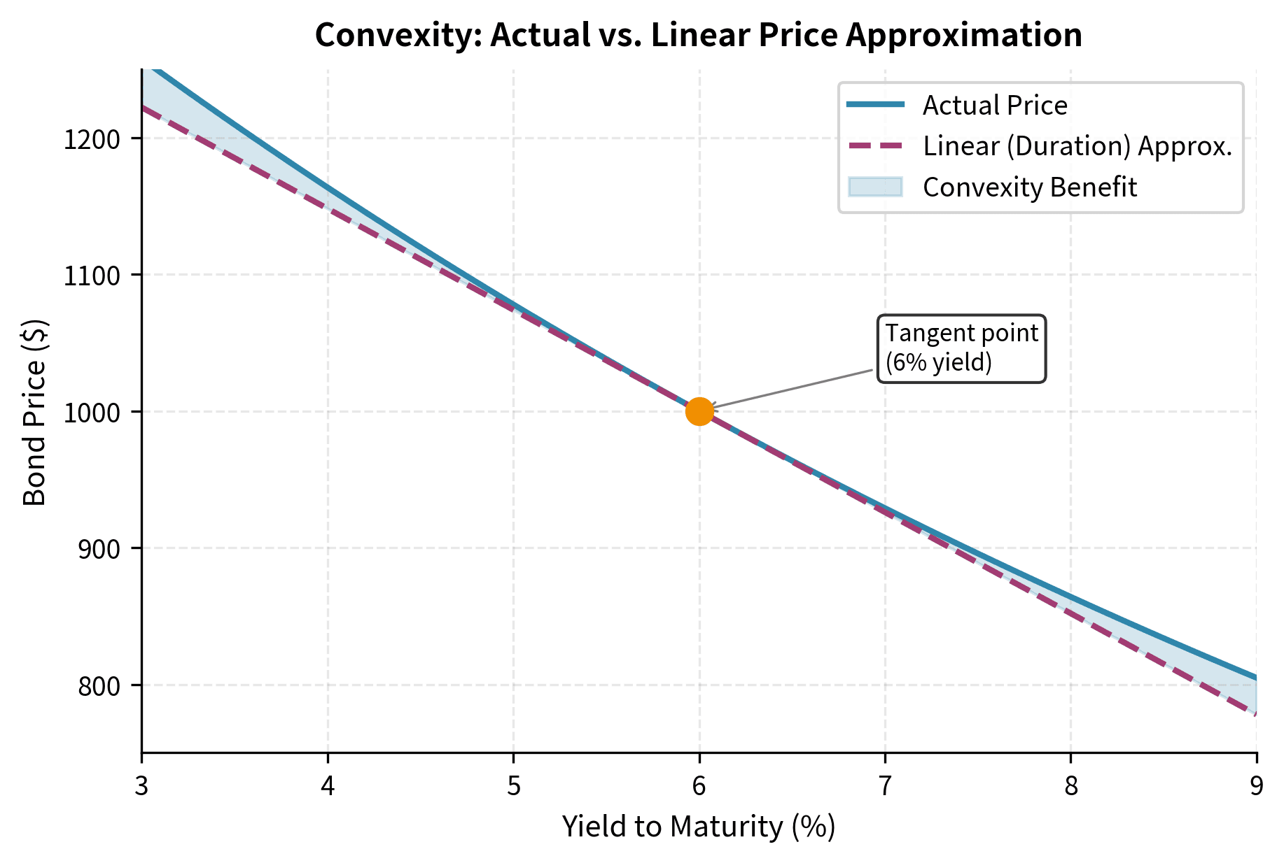
This convexity effect becomes more pronounced for bonds with longer maturities and lower coupons, as we'll explore when discussing duration and convexity in subsequent chapters.
Practical Example: Comparing Bond Investments
Let's apply these concepts to compare two bonds and determine which offers better value. Consider an investor choosing between:
- Bond A: 5-year maturity, 4% coupon, priced at $950
- Bond B: 5-year maturity, 6% coupon, priced at $1,040
Bond A's yield to maturity of approximately 5.2% exceeds Bond B's yield of approximately 5.1%. Despite Bond B having a higher coupon and greater total cash flows, Bond A offers the higher yield to maturity. This is because Bond A trades at a deeper discount, and its price appreciation to par provides additional return. The YTM captures this total return, making it the appropriate comparison metric.
The current yield (annual coupon divided by price) can be misleading because it ignores price appreciation for discount bonds and price depreciation for premium bonds.
Limitations and Practical Considerations
Bond pricing in practice involves complexities beyond this simplified framework. Understanding these limitations helps practitioners apply theoretical models appropriately.
The assumption of a single discount rate (the YTM) for all cash flows is a significant simplification. In reality, interest rates vary by maturity, forming a yield curve. Short-term rates may differ substantially from long-term rates, and using a single rate ignores this term structure. More sophisticated approaches discount each cash flow at its own appropriate rate, a topic we'll address when discussing yield curve construction.
Credit risk adds complexity for non-government bonds. The probability that an issuer defaults on payments affects bond prices, but this probability changes over time with the issuer's financial condition and macroeconomic factors. Models that assume constant credit spreads fail to capture this dynamic risk. Furthermore, bonds often include embedded options, such as call provisions that let the issuer redeem bonds early or put provisions that let investors sell bonds back to the issuer. These options affect cash flow timing and require option-adjusted analysis.
Liquidity also influences prices. A bond that trades infrequently may have a wider bid-ask spread and a price that doesn't fully reflect current market conditions. Two bonds with identical cash flows may trade at different prices simply because one is more liquid than the other.
Despite these limitations, the discounted cash flow framework remains the foundation of bond analysis. Understanding this framework is essential before tackling more advanced topics like duration, convexity, and term structure models.
Summary
This chapter established the fundamental concepts for understanding and pricing bonds:
Bond Characteristics: Bonds are defined by their face value, coupon rate, maturity, payment frequency, and issuer. Government bonds serve as risk-free benchmarks, while corporate bonds carry credit spreads reflecting default risk.
Pricing Framework: Bond prices equal the present value of future cash flows. For coupon bonds, this involves discounting both the annuity of coupons and the face value at maturity. Zero-coupon bonds involve a single discounted cash flow.
Yield to Maturity: The YTM is the single rate that equates a bond's price to its cash flows. It provides a standardized comparison measure but assumes reinvestment at the same rate and holding to maturity.
Fixed vs. Floating Rate: Fixed rate bonds have constant coupons, making their prices sensitive to interest rate changes. Floating rate bonds have coupons that reset periodically, keeping prices near par.
Clean and Dirty Prices: Markets quote clean prices for comparability, but transactions settle at dirty prices that include accrued interest. Day count conventions determine how accrued interest is calculated.
Price-Yield Relationship: Prices and yields move inversely, with the relationship exhibiting positive convexity that benefits bondholders through asymmetric price responses to yield changes.
Key Parameters
The key parameters for bond pricing and analysis are:
-
Face Value (F): The principal amount repaid at maturity. Serves as the baseline for calculating coupon payments and determines the bond's par value.
-
Coupon Rate (c): The annual interest rate applied to face value. Higher coupon rates mean larger periodic cash flows and less price sensitivity to yield changes.
-
Years to Maturity (T): Time until the bond matures. Longer maturities increase both the number of cash flows and the bond's sensitivity to interest rate changes.
-
Yield to Maturity (y): The discount rate that equates price to present value of cash flows. Represents the total return if held to maturity with reinvestment at the same rate.
-
Payment Frequency (m): Number of coupon payments per year. Affects compounding calculations. Semiannual payments use y/2 as the periodic rate.
-
Reference Rate: For floating rate bonds, the benchmark rate (e.g., SOFR) that determines coupon resets. Changes in this rate directly affect future coupon payments.
-
Spread: The fixed margin over the reference rate for floating rate bonds. Reflects the issuer's credit risk and remains constant throughout the bond's life.
Quiz
Ready to test your understanding? Take this quick quiz to reinforce what you've learned about bond fundamentals and pricing.

Comments