Predicting Model Performance: Scaling Laws & Forecasting

The scaling laws we've developed in previous chapters reveal a powerful property: language model performance follows predictable mathematical relationships. But the true value of these relationships lies not in explaining past results; it lies in predicting future ones. If we can forecast how a model will perform before spending millions of dollars training it, we can make better decisions about architecture choices, compute allocation, and research direction.

This predictive power changes the economics of AI research. Instead of treating each training run as an expensive experiment with uncertain outcomes, we can approach model development more like engineering. We can specify requirements, predict what resources will achieve them, and make informed trade-offs before committing to them. The ability to look ahead, even imperfectly, moves research planning from educated guesswork toward quantitative analysis.

This chapter turns scaling laws from descriptive tools into predictive instruments. We'll examine how to extrapolate loss curves, the challenges of predicting downstream capabilities, techniques for quantifying prediction uncertainty, and the conditions under which these forecasts remain reliable. Predicting model performance is both more tractable and more subtle than it first appears.

The most direct application of scaling laws is predicting the test loss a model will achieve at a given scale. This prediction task asks a simple question: if we train a model with $N$ parameters on $D$ tokens of data, what loss should we expect? The answer comes from the mathematical relationships we've established between scale and performance.

From the Chinchilla scaling law we covered in Part XXI, Chapter 3, we know that loss follows:

To understand what this formula captures, let's examine each component and the intuition behind the mathematical structure:

• $L(N, D)$: the predicted test loss for a model with $N$ parameters trained on $D$ tokens
• $N$: the number of model parameters (capturing model capacity)
• $D$: the number of training tokens (capturing data scale)
• $E$: the irreducible loss, the theoretical minimum achievable even with infinite compute, determined by the entropy of natural language
• $A$: the parameter scaling coefficient, controlling how much model size reduces loss
• $B$: the data scaling coefficient, controlling how much training data reduces loss
• $\alpha$: the parameter scaling exponent (typically ~0.34), determining how quickly returns diminish as models grow
• $\beta$: the data scaling exponent (typically ~0.28), determining how quickly returns diminish as data grows

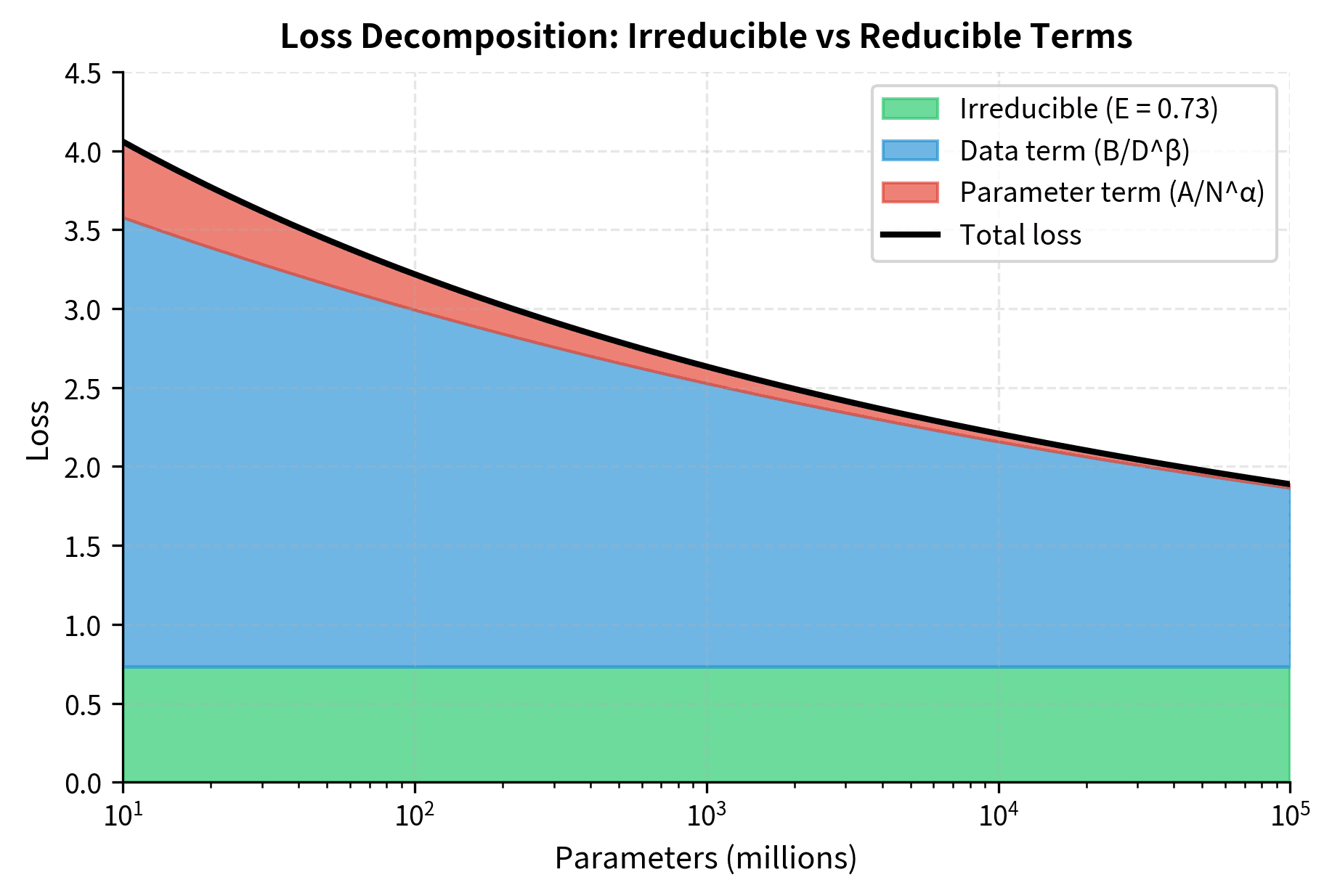
The formula captures an important property: loss decomposes into three independent terms, each telling us something different about where performance comes from and what limits it. The irreducible loss $E$ sets a floor that no amount of scaling can breach. This represents the fundamental unpredictability in language itself, the entropy that remains even when we know all the patterns. If someone asks "What word comes next?", sometimes multiple words are genuinely plausible, and no model can do better than chance on these cases.

The power-law terms $A/N^{\alpha}$ and $B/D^{\beta}$ represent reducible error that diminishes as we scale, but with diminishing returns governed by the exponents. The mathematical form of power laws encodes a crucial property: each doubling of scale produces a constant fractional improvement rather than a constant absolute improvement. When $\alpha = 0.34$, doubling model size reduces the parameter-dependent loss term by a factor of $2^{0.34} \approx 1.27$, or roughly 21%. This same 21% reduction applies whether we're going from 1B to 2B parameters or from 100B to 200B. The absolute loss reduction shrinks, but the proportional improvement remains constant.

The additive structure, simply summing the three terms, reflects an important empirical finding: the contributions from model size and data size appear to be approximately independent. A larger model benefits equally from more data regardless of its starting size, and more data helps equally regardless of model capacity. This separability is what makes extrapolation tractable; if the terms interacted in complex ways, prediction would require understanding those interactions at scales we haven't tested.

Given these fitted parameters, extrapolating to larger scales seems straightforward: plug in your target $N$ and $D$, compute $L$. However, the practical challenge lies in fitting these parameters reliably from limited training runs. We need enough data points to constrain a five-parameter model, but we're typically trying to minimize how many expensive training runs we perform.

The standard approach trains a series of models at small scales, measures their final losses, then fits the scaling law parameters. The key insight is that the exponents $\alpha$ and $\beta$ appear stable across model families, so we primarily need to estimate the coefficients. This stability helps. It means that even if our small-scale experiments can't pin down the exponents exactly, we can borrow values from published research on similar architectures and focus our fitting effort on the coefficients that capture our specific training setup.

The fitting process treats our scaling law as a regression problem: we have observed data points (pairs of scale and achieved loss) and want to find parameters that best explain those observations. The nonlinear form of the power laws requires iterative optimization rather than closed-form solutions, but modern optimization libraries handle this efficiently.

The fitted parameters reveal the structure of our scaling relationship. The irreducible loss $E$ represents the theoretical minimum achievable with infinite compute, determined by the entropy of natural language itself. When we fit this parameter, we're essentially asking: "If we extrapolate the trend of diminishing returns to infinity, where does it asymptote?" The answer gives us a sense of how close we are to fundamental limits and how much room for improvement remains.

The coefficients $A$ and $B$ capture the "magnitude" of each scaling dimension's contribution. Larger coefficients mean that dimension has more reducible error, more room for improvement. The ratio between them indicates the relative importance of model size versus data size for our particular training setup.

The exponents $\alpha$ and $\beta$ quantify how quickly performance improves as we scale each dimension. The asymmetry between them (typically $\alpha > \beta$) suggests that parameter scaling has slightly better returns than data scaling, though both exhibit strong diminishing returns. These exponents determine the steepness of our improvement curve: larger exponents mean faster initial gains but also faster saturation.

With fitted parameters in hand, we can now predict performance at scales we haven't trained. This is where scaling laws earn their keep, transforming expensive experiments into inexpensive calculations. The prediction itself is just arithmetic: substitute our target values into the fitted formula. But understanding what we're doing mathematically helps us appreciate both the power and the limitations of this extrapolation.

When we plug in a target $N$ and $D$, we're asserting that the functional relationship we observed at small scales continues to hold at large scales. We're assuming that the same three-term structure, irreducible loss plus two power-law improvements, captures the physics of learning at 70 billion parameters just as well as at 70 million. This is a strong assumption, and one we can never fully verify without actually training the larger model.

These predictions extrapolate 1-2 orders of magnitude beyond our training data. The further we extrapolate, the more our predictions depend on the assumption that scaling relationships remain stable, an assumption we'll examine critically later in this chapter. This extrapolation gives us significant leverage. We use models that cost thousands of dollars to train in order to predict the behavior of models that cost millions of dollars. This leverage explains why this technique has become central to AI research planning.

A visual representation helps build intuition for what extrapolation means geometrically. The scaling law defines a surface in three-dimensional space, where two dimensions represent our inputs (parameters and tokens) and the third dimension represents the output (loss). Our training data points lie somewhere on this surface, and fitting the scaling law means finding the surface that best passes through them. Extrapolation asks: if we extend this surface beyond where we have data, what does it predict?

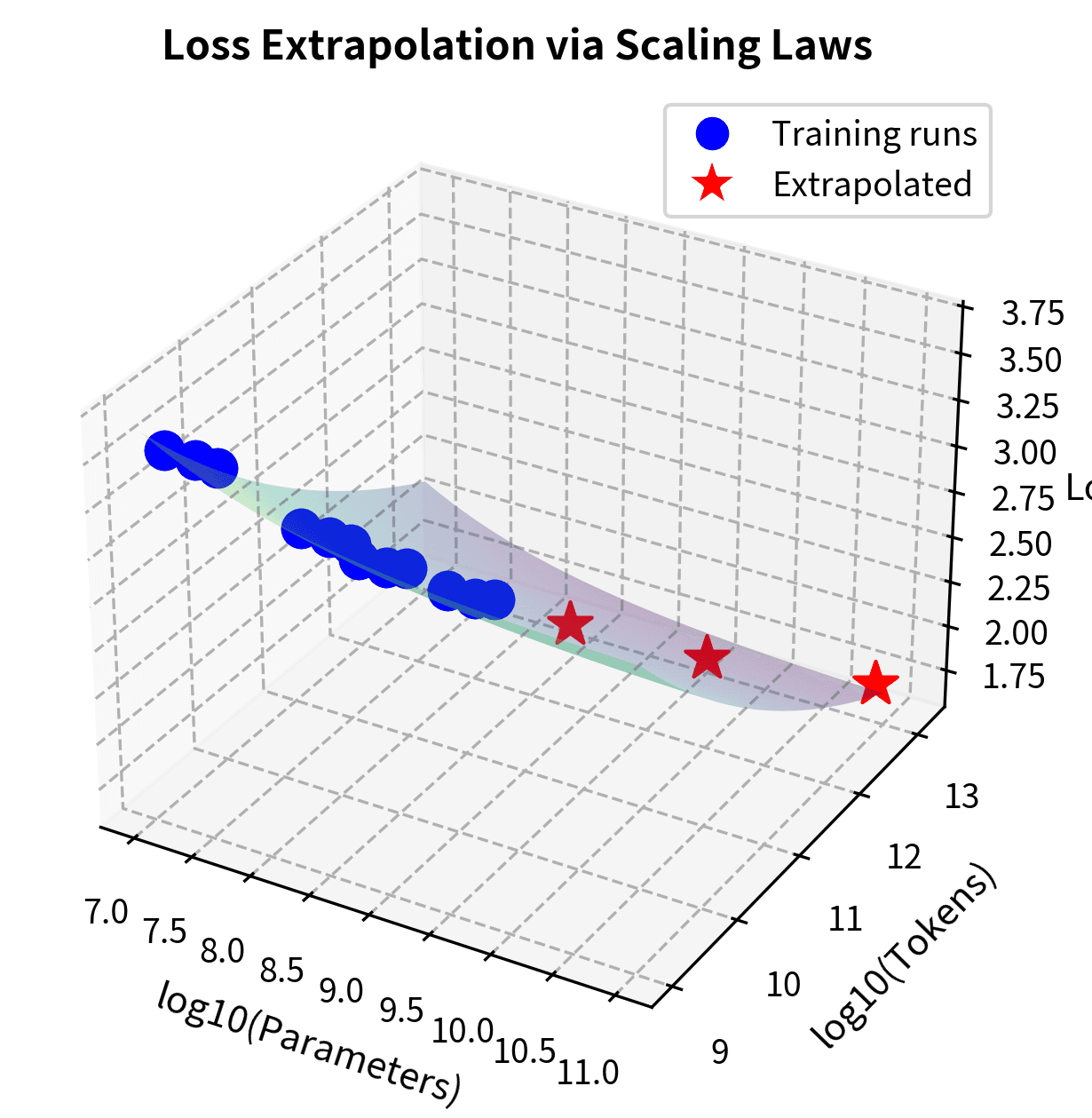
The surface in @fig-loss-extrapolation shows how loss decreases as we move along either scaling dimension. The curvature of the surface reflects the diminishing returns encoded in our power-law exponents. Improvement slows as we push further along either axis. Our extrapolated predictions (red stars) assume this smooth surface continues beyond observed data, a reasonable assumption given empirical evidence, but one that carries increasing uncertainty at extreme scales. Notice how the red stars sit far from the blue cluster of training points, making visually concrete just how much we're extending beyond our empirical grounding.

Predicting loss is useful for comparing training efficiency, but practitioners care about what models can do. Can a 70B model solve math problems? Will a 7B model follow complex instructions? Connecting loss predictions to capability predictions introduces significant challenges that go beyond the mathematical smoothness of loss curves.

The fundamental difficulty is that loss and capabilities measure different things. Loss is a continuous quantity that summarizes average prediction quality across millions of tokens. Capabilities are often binary or threshold-based: either the model can do the task or it can't. Bridging this gap requires understanding the relationship between average performance and specific task success, a relationship that can be highly nonlinear.

Test loss measures how well a model predicts the next token on average. Capabilities measure whether a model can perform specific tasks. These tasks often require chains of correct predictions or reasoning steps that loss doesn't directly capture. This distinction matters because a model could have excellent loss while failing at tasks that require sustained accuracy. Conversely, it could succeed at tasks despite mediocre average loss if it excels in the right places.

Mathematically, test loss is the cross-entropy averaged over all tokens:

Let's unpack what each symbol means and why this formula captures prediction quality:

• $L$: the average loss across all tokens
• $T$: the total number of tokens in the test set
• $x_t$: the $t$-th token in the sequence
• $x_{<t}$: all tokens preceding position $t$ (the context)
• $P(x_t \mid x_{<t})$: the model's predicted probability for the correct token given the context

The negative sign and logarithm work together in a specific way: when the model assigns high probability to the correct token, $\log P$ is close to zero (a small negative number, so the negative of it is a small positive number, a small penalty). When probability is low, $\log P$ becomes a large negative number, so the negative gives a large positive penalty. The logarithm is essential here because it makes the loss additive across independent predictions and penalizes confident wrong predictions more severely than uncertain ones.

Averaging over all tokens gives the mean prediction quality across the entire test set. This averaging is both a strength and weakness of loss as a metric. It's a strength because it provides a stable, comprehensive measure that doesn't depend on which specific tokens we choose to examine. It's a weakness because the averaging obscures capability-relevant structure: a model might predict common words perfectly (low contribution to loss) while struggling with the rare but critical tokens that determine task success.

Consider two hypothetical scenarios for a math problem where the final answer is a specific token:

• Model A predicts the correct answer token with 20% probability (wrong most of the time when sampling, contributing to higher loss)
• Model B predicts it with 52% probability (right most of the time if we take the argmax)

The loss difference between these scenarios is modest, both models are far from certain. For Model A, the loss contribution from this token is $-\log(0.20) \approx 1.61$. For Model B, it's $-\log(0.52) \approx 0.65$. The difference of about 1 nat seems significant but represents just one token among thousands. Yet the capability difference is binary: Model A usually gets the answer wrong, Model B usually gets it right. This nonlinear relationship between loss and task success creates prediction challenges that no amount of loss extrapolation can fully address.

As we'll discuss in Part XXII on emergence, some capabilities appear suddenly as models scale rather than improving gradually with loss. This creates a limitation for extrapolation. If a capability is absent at all scales we've tested, we can't reliably predict when it will appear. The capability might emerge at the next doubling of scale, or it might require ten more doublings. Loss trends alone don't tell us.

Emergence often follows a sigmoid pattern rather than a power law. While loss decreases smoothly following $L \propto N^{-\alpha}$, capabilities can transition from near-zero to near-perfect over a relatively narrow range of scales. Understanding this sigmoid pattern helps us recognize why capability prediction is fundamentally harder than loss prediction.

The sigmoid function's mathematical properties explain why emergence feels sudden. The steepness parameter $k$ controls how rapidly the transition occurs: when $k$ is large, the function jumps quickly from near-zero to near-one. In log-scale (which is how we typically view model sizes), a steep sigmoid means that capability jumps from negligible to saturated over perhaps a single order of magnitude in scale. If our training runs span models from 10M to 300M parameters, and the transition happens around 1B, we see nothing but flat near-zero performance, giving no warning of the imminent jump.

@fig-capability-emergence illustrates the challenge: while loss (left) decreases smoothly and predictably with scale, capabilities (right) can exhibit sharp transitions. The left panel shows the gentle, monotonic curve that scaling laws capture well. Each doubling of scale yields a predictable improvement. The right panel shows a fundamentally different pattern: near-zero performance persists across multiple scale doublings, then capability rapidly emerges, then saturates near perfect. If we only have data from scales below 500M parameters, the capability curve appears nearly flat, giving no indication of the imminent jump. This is not a failure of our fitting procedure. It's a property of threshold-based capabilities.

For tasks that improve more gradually with scale, we can attempt direct prediction using transfer functions from loss to accuracy. The important observation is that accuracy often improves linearly with improvements in log-loss rather than raw loss. This makes intuitive sense. Reducing loss from 4.0 to 2.0 (a halving) is a much bigger deal than reducing from 2.0 to 1.5, even though the absolute reduction is smaller. The logarithmic relationship captures how capability gains become harder to achieve as performance improves.

The transfer function's structure encodes important assumptions about how capabilities emerge from improved language modeling. The baseline parameter captures the performance of a random guesser, for four-way multiple choice, this is 25%. The ceiling is the loss at which models perform no better than random. Below this loss, capability begins to emerge. The floor is the loss at which capability saturates near 100%. Between ceiling and floor, we interpolate linearly in log-loss space.

This parameterization requires calibration data: we need to have observed models across a range of losses on each specific task to fit the ceiling and floor values. Different tasks have different calibrations because they depend on loss in different ways. A task requiring rare factual knowledge might need very low loss before accuracy improves, while a task testing common patterns might show improvement at higher loss.

These capability predictions rely on task-specific calibration curves fit from previous evaluations. The accuracy improves only as quickly as the underlying calibration data allows. If we've never seen models with loss below 2.0 on a task, we're extrapolating the loss-accuracy relationship as well as the loss itself. This compounds the uncertainty: we're extrapolating one uncertain prediction through another uncertain function.

Any prediction is incomplete without uncertainty bounds. Scaling law predictions face several sources of uncertainty that compound as we extrapolate further. Understanding and quantifying this uncertainty is essential for sound decision-making. A prediction of loss 2.0 with uncertainty ±0.1 means something very different from the same prediction with uncertainty ±0.5.

The sources of uncertainty fall into two broad categories. First, there's parameter uncertainty: our fitted parameters are estimates based on noisy data, and different training runs might yield slightly different fits. Second, there's model uncertainty: the scaling law functional form itself is an approximation that might break down at extreme scales. Both types of uncertainty grow as we extrapolate further from observed data.

The fitted parameters have uncertainty, captured in the covariance matrix from our optimization. When we fit a nonlinear model like the scaling law, the optimization process estimates the best-fit parameters and how much those estimates might vary given the noise in our data.

The covariance matrix encodes this uncertainty. It's a symmetric matrix where diagonal elements represent the variance of each parameter (how much that parameter's estimate might fluctuate if we repeated the fitting with different data), and off-diagonal elements capture how parameter uncertainties correlate (if one parameter is estimated too high, is another likely to be estimated too high or too low?). These correlations matter for prediction because errors in different parameters can either compound or cancel.

The relative errors reveal which parameters are best-constrained by our data. Parameters with smaller relative errors are more reliably estimated, while those with larger relative errors contribute more uncertainty to predictions. Typically, the exponents $\alpha$ and $\beta$ have higher relative uncertainty because power-law exponents are inherently difficult to estimate exactly. Small changes in the exponent create large changes in the prediction at extreme scales.

These uncertainties propagate through our predictions via error propagation. The mathematical challenge is that our scaling law is a nonlinear function of the parameters, so we can't simply add uncertainties in quadrature as we might for a linear model. Instead, we use Monte Carlo sampling: generate many sets of plausible parameters from the fitted distribution, compute predictions for each, and examine the spread of results.

The Monte Carlo approach has a clear interpretation: we're asking "given everything we know about parameter uncertainty, what range of predictions is plausible?" Each sample represents a possible true state of the world consistent with our observations. The spread of predictions across samples reflects our genuine uncertainty about the outcome.

Uncertainty grows with extrapolation distance. A useful heuristic tracks how far beyond training data we're predicting. This growth isn't arbitrary. It reflects a mathematical property: the further we extrapolate, the more our predictions depend on the precise values of parameters we've estimated imperfectly, and small errors in those parameters translate to larger errors in predictions.

The relationship between extrapolation distance and uncertainty isn't linear. Near our training data, even moderate parameter uncertainty produces tight predictions because all parameter sets agree closely. Far from training data, the fan-out effect appears: different parameter sets that all fit the training data equally well can diverge dramatically in their extrapolated predictions. This is especially true for the exponents, where a small difference (say, 0.34 vs 0.36) makes little difference at $N = 10^8$ but substantial difference at $N = 10^{11}$.

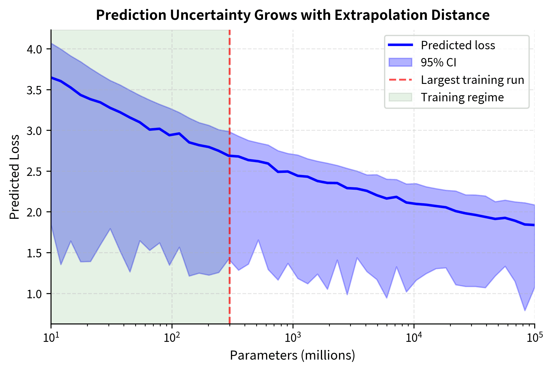
@fig-uncertainty-growth shows a critical pattern: within the training regime (green shading), predictions are well-constrained with tight confidence bands. Beyond our largest training run (red line), confidence intervals expand rapidly. The shaded region fans out as we push into unexplored territory. This visual representation helps calibrate how much trust to place in extrapolated predictions. A prediction at 1B parameters might be reliable enough to bet on; a prediction at 100B parameters should be treated as indicative rather than definitive.

Beyond parameter uncertainty, there's model uncertainty. The scaling law functional form itself might not hold at extreme scales. Model uncertainty is harder to quantify because it involves questioning assumptions that underlie the approach. Parameter uncertainty asks "given that the scaling law is correct, what's our uncertainty in the prediction?" Model uncertainty asks "what if the scaling law itself is wrong?"

Several approaches help assess model uncertainty:

Holdout validation: Fit on smaller runs, predict on largest held-out runs. This tests the key extrapolation scenario: can we predict performance of models larger than those used for fitting? The errors on holdout data give an empirical estimate of extrapolation accuracy within our observed range.

Functional form comparison: Compare predictions from different scaling law variants. If the Chinchilla form, the OpenAI form, and other variants all agree at some scale, we have more confidence; if they diverge, we know model uncertainty is significant.

Domain expertise: Physics-based constraints can bound plausible loss values. The irreducible loss $E$ can't be negative. Loss can't drop below certain information-theoretic limits. These constraints don't quantify uncertainty but can flag implausible predictions.

The holdout validation gives us an empirical estimate of how well our scaling law extrapolates within the observed range. The mean absolute error tells us typical prediction accuracy in absolute terms. The bias reveals systematic tendencies: positive bias indicates our predictions are optimistic (actual loss is lower than predicted, meaning models perform better than expected), while negative bias indicates pessimism (models underperform predictions). Understanding the direction of bias helps calibrate expectations and make appropriately conservative or aggressive decisions.

When can we trust scaling law predictions? Several conditions affect reliability. Understanding these conditions helps practitioners know when to rely heavily on predictions and when to treat them as rough guides requiring empirical verification.

Scaling law predictions are most reliable when:

1. Training conditions remain constant. The scaling laws assume consistent training procedures, including similar architectures, hyperparameters, data distributions, and optimization strategies. Changes to any of these can shift the scaling curves. A scaling law fit on GPT-style autoregressive models won't accurately predict T5-style encoder-decoder models. Similarly, changing from AdamW to a different optimizer, or from standard attention to flash attention, can introduce systematic offsets. This doesn't make predictions useless; the slopes often remain similar, but the intercepts can shift.

2. Extrapolation is limited. Predictions within 10× of training data are generally reliable. Predictions beyond 100× are speculative. The Chinchilla paper fit on models up to 16B parameters, yet predictions for 70B models proved reasonably accurate, though this represented only ~5× extrapolation. A rule of thumb is to treat the uncertainty as roughly doubling for each order of magnitude of extrapolation beyond the training regime.

3. The capability doesn't exhibit phase transitions. Smoothly improving capabilities like perplexity and HellaSwag accuracy extrapolate better than emergent capabilities like chain-of-thought reasoning. Before attempting capability prediction, examine whether existing data shows smooth trends or hints of nonlinear behavior. Smooth trends at small scale suggest (but don't guarantee) smooth behavior at large scale.

4. Data quality is maintained. Scaling laws fit on high-quality data don't transfer to low-quality data. As training datasets grow, maintaining quality becomes increasingly difficult. This creates a source of systematic prediction error. If you're fitting on carefully curated data but will train the final model on noisier data due to volume requirements, predictions will be systematically optimistic.

The track record of scaling law predictions provides calibration for future forecasts. Examining cases where predictions succeeded and failed helps us understand reliability in practice:

These examples show that predictions within ~5% are achievable for moderate extrapolation factors. The Chinchilla prediction was remarkably accurate at only 4× extrapolation. Even GPT-3, with 12× extrapolation, came within 3% of prediction. However, this historical accuracy reflects models trained under similar conditions to the scaling law fits. Novel architectures or training procedures can produce larger deviations. The track record supports confidence but not overconfidence.

Scaling law predictions fail systematically in several scenarios:

Architecture discontinuities. The transition from attention mechanisms to linear attention, or from dense to sparse (MoE) models, introduces new scaling relationships. Predictions fit on dense transformers don't transfer to MoE models without refitting. MoE models have different effective parameter counts and different compute-performance relationships. Each architecture requires its own scaling study.

Data exhaustion. When models train on all available high-quality data and must use lower-quality sources, performance degrades faster than loss-based scaling laws predict. The scaling law assumes infinite high-quality data, but reality imposes constraints that scaling laws don't capture. As training corpora grow larger, data quality and diversity become binding constraints that idealized scaling laws don't capture.

Capability phase transitions. Some capabilities emerge suddenly, as we'll examine in Part XXII. No amount of loss extrapolation predicts these transitions from first principles. If a capability hasn't appeared at any scale you've tested, loss trends provide no guidance about when it might emerge.

Optimization instabilities. Larger models encounter training instabilities that smaller models don't. Loss spikes and training divergence aren't captured in smooth scaling laws, which assume successful training. A prediction that 100B parameters will achieve loss 1.9 doesn't account for the possibility that training at that scale proves unstable and requires restarts, different hyperparameters, or architectural modifications.

Given these techniques and caveats, how should practitioners approach performance prediction in real projects? The goal is to balance prediction value against its costs and integrate predictions into decision-making rather than treating them as ground truth.

A practical workflow uses progressively larger "stepping stone" models. The idea is to invest a small fraction of the total training budget in preliminary runs that provide data for fitting scaling laws with decreasing extrapolation distance. Each rung of the ladder gives us more confidence in our prediction for the final run.

This ladder approach invests a small fraction of the total compute budget in preliminary runs that inform the final training decision. The geometric spacing ensures coverage across scales while keeping total ladder cost bounded. Each run provides data points for fitting scaling laws with decreasing extrapolation distance. By the time we've completed the ladder, we're extrapolating perhaps 30× rather than 1000×.

The ladder also provides early warning of problems. If the scaling relationship looks anomalous at intermediate scales, perhaps due to architectural issues or data problems, we discover this cheaply before committing to the full run.

With predictions and uncertainties in hand, teams can make informed decisions. The goal is to translate raw predictions into information that supports go/no-go decisions and resource allocation:

This framework translates raw predictions into actionable information: the probability of achieving targets, expected benchmark performance, and confidence levels. Decision-makers can then weigh these forecasts against compute costs and alternative investments. A 60% probability of hitting a loss target might justify a go-ahead for a moderate-cost run but not for an extremely expensive one. The framework makes trade-offs explicit and quantitative.

Scaling law prediction has reshaped AI research planning, but its value depends on understanding both what it enables and where it falls short. This section examines the fundamental constraints on prediction accuracy and the practical impact these forecasting methods have had on the field.

Scaling law prediction faces inherent limits that no amount of methodological refinement can overcome. Acknowledging these limits enables appropriate use of the methods.

Irreducible uncertainty from emergence. When capabilities emerge discontinuously, predictions based on loss extrapolation miss the phenomenon. The emergence of chain-of-thought reasoning in sufficiently large models wasn't predicted by scaling laws; it was discovered empirically. This suggests that some important capabilities may be those we cannot forecast. Scaling laws predict "more of the same, but better." They don't predict "qualitatively new."

Distributional shift in training data. Scaling laws assume the data distribution remains constant. As models consume ever-larger training corpora, training datasets inevitably include data of varying quality, domain coverage, and temporal distribution. These shifts introduce prediction errors that compound with scale. A model trained on 10T tokens will necessarily draw from different sources than a model trained on 100B tokens, and scaling laws don't capture how that difference affects performance.

Architecture evolution. Scaling laws are fit to specific architectures. The transition from LSTM to Transformer made prior scaling work obsolete. The Transformer had different scaling properties that couldn't be predicted from LSTM data. Future architectural innovations, whether sparse attention, state space models, or other approaches, will similarly require new scaling relationships. Predictions assume the current architecture extends indefinitely, which history suggests is unrealistic.

Optimization limits. Larger models require modified training procedures: different learning rate schedules, initialization schemes, and stability measures. These modifications aren't captured in idealized scaling laws but materially affect achieved performance. A scaling law that assumes perfect optimization may overestimate what's achievable when training at scale proves difficult.

Despite these limitations, scaling law prediction has changed how organizations approach large model development.

Resource allocation. Organizations now estimate compute requirements for target capabilities with reasonable precision, enabling informed decisions about multi-million dollar training runs. Before scaling laws, training large models involved substantial guesswork; now it's a calculated risk with quantified uncertainty.

Research prioritization. Predictions help identify when algorithmic improvements outpace scaling. If a technique beats the scaling curve, it merits investigation. Conversely, if returns are merely matching scaling predictions, scaling itself may be the more efficient path. This comparison between "scale up what works" and "find something better" is central to research strategy.

Timeline forecasting. The AI research community uses scaling predictions to estimate when certain capability levels become achievable, informing policy discussions and safety research priorities. While these forecasts carry uncertainty, they provide a quantitative basis for planning that vague intuitions don't.

Competitive intelligence. Published scaling laws allow rough inference of what competitors might achieve with known compute resources, informing strategic decisions. If a competitor has 10× your compute budget, scaling laws tell you roughly how much better their models will be. This information helps with positioning and investment decisions.

The limitations are calibration factors to incorporate, not obstacles to dismiss. A 10% prediction error on loss might translate to much larger uncertainty on specific capabilities. Wise use of scaling predictions acknowledges this uncertainty while still extracting valuable guidance. The alternative, making expensive decisions with no quantitative forecasting at all, is worse.

Predicting model performance turns scaling laws from retrospective analysis into prospective planning tools:

Loss extrapolation uses fitted scaling laws to predict test loss at untrained scales, with accuracy typically within 5-10% for moderate extrapolation factors.

• Capability prediction is harder than loss prediction because task success often exhibits phase transitions rather than smooth improvement
• Uncertainty quantification through parameter sampling, holdout validation, and model comparison provides confidence bounds essential for decision-making
• Prediction reliability depends on stable training conditions, limited extrapolation distance, smoothly-improving capabilities, and maintained data quality
• Practical workflows use scaling ladders, small training runs that inform predictions before committing to expensive final training

The tension in performance prediction is that the capabilities we most want to forecast, novel emergent abilities, are those that scaling laws fail to predict. Loss extrapolation works well because loss improves smoothly; capabilities can jump discontinuously.

Yet even imperfect predictions affect research economics. Knowing that a 70B model will likely achieve 2.1 loss rather than 2.5 loss, even with 10% uncertainty, justifies or rules out billion-dollar training investments. The next chapter on emergence will examine why some capabilities resist prediction entirely, and what that implies for the future of capability forecasting.

The parameters for scaling law prediction are:

• E (irreducible loss): The theoretical minimum loss achievable with infinite compute, determined by the entropy of natural language.
• A, B (scaling coefficients): Control how much model size and data size reduce loss respectively.
• α, β (scaling exponents): Determine how quickly returns diminish as each dimension scales (typically ~0.34 and ~0.28).
• n_samples: Number of Monte Carlo samples for uncertainty quantification. More samples provide tighter confidence intervals.
• holdout_fraction: Fraction of largest training runs to reserve for validation when testing extrapolation accuracy.

Ready to test your understanding? Take this quick quiz to reinforce what you've learned about predicting model performance using scaling laws.