

Learn T5's encoder-decoder architecture, relative position biases, span corruption pretraining, and text-to-text framework for unified NLP tasks.

This article is part of the free-to-read Language AI Handbook
Choose your expertise level to adjust how many terms are explained. Beginners see more tooltips, experts see fewer to maintain reading flow. Hover over underlined terms for instant definitions.
T5 Architecture
The Text-to-Text Transfer Transformer (T5) introduced a unifying framework for natural language processing: treat every task as text generation. Translation, summarization, question answering, and classification all become the same problem of mapping input text to output text. This simple approach allowed researchers to study what matters most for transfer learning at scale.
Released by Google Research in 2019, T5 emerged from a systematic exploration of pre-training techniques, model architectures, and scaling strategies. The accompanying paper, "Exploring the Limits of Transfer Learning with a Unified Text-to-Text Transformer," tested dozens of design choices to identify which ones actually matter. The result was both a powerful model family and a practical guide to building better language models.
T5's encoder-decoder architecture handles both understanding and generation in a single model. The encoder processes the full input with bidirectional attention, while the decoder generates output autoregressively. This design excels at tasks requiring deep comprehension of the input before producing structured output, making T5 particularly effective for translation, summarization, and question answering.
The Text-to-Text Framework
T5's central insight is that natural language provides a universal interface for NLP tasks. Instead of building task-specific architectures with specialized output heads, T5 learns to generate the answer as text. This means the same model, loss function, and training procedure work for any task.
To appreciate why this matters, consider how NLP systems were traditionally built. Classification tasks required a final layer that mapped hidden representations to a fixed set of class probabilities. Question answering systems needed span prediction heads that identified start and end positions in text. Translation models required sequence-to-sequence architectures with dedicated vocabulary handling for each language pair. Each task demanded its own architectural modifications, training objectives, and output processing logic.
The text-to-text framework eliminates these distinctions by building on an insight: natural language is already a universal representation system. Humans express classification decisions ("this is negative"), answer questions ("the color is blue"), and produce translations ("Das Haus ist wunderbar") all through the same medium, text. If we train a model to be exceptionally good at generating text, it can express any answer we might need.
A framework where all NLP tasks are cast as text generation problems. The model receives text input (with a task prefix) and produces text output, eliminating the need for task-specific architectures.
Consider how different tasks map to this framework:
- Translation:
translate English to German: The house is wonderful.→Das Haus ist wunderbar. - Summarization:
summarize: [long article text]→[concise summary] - Classification:
sentiment: This movie was terrible.→negative - Question answering:
question: What color is the sky? context: The sky appears blue during the day.→blue
The task prefix tells the model what to do, and the target text encodes the answer. Classification becomes generating the class label as a word. Regression could output the number as text. Even complex structured outputs like parse trees can be serialized as strings.
This uniformity has practical benefits. You can fine-tune a single model on multiple tasks simultaneously. You can add new tasks without changing the architecture. You can also leverage text generation advances, like beam search and nucleus sampling, across all applications.
Encoder-Decoder Architecture
T5 uses the original Transformer's encoder-decoder structure, with modifications that improve training stability and performance. This architectural choice reflects an insight about how different NLP tasks process information. Some tasks, like classification or sentiment analysis, primarily require understanding an input. Others, like open-ended writing, primarily require generating new content. But many of the most challenging tasks, translation, summarization, and question answering, require both: deep comprehension of the input followed by structured generation of output. The encoder-decoder architecture provides dedicated machinery for each phase of this process.
The encoder processes the input sequence bidirectionally, creating rich contextual representations where each token's embedding reflects its relationships with every other token in the input. The decoder then generates output tokens one at a time, attending to both the encoder's output and its own previous predictions. This separation allows the encoder to build a complete understanding of the source text before the decoder begins generating, ensuring that even the first output token benefits from full context about the input.
Encoder Structure
The encoder consists of stacked Transformer blocks, each containing self-attention and feed-forward layers. Unlike GPT-style decoders, the encoder uses bidirectional attention. Every token can attend to every other token in the input, regardless of position. This bidirectionality is crucial for tasks like translation and summarization, where understanding a word often requires seeing what comes both before and after it. Consider the sentence "The bank was steep." Determining whether "bank" refers to a financial institution or a riverbank requires seeing "steep," which comes later in the sequence.
Each encoder block applies a carefully orchestrated sequence of operations that transform token representations while maintaining training stability:
- Layer normalization (applied before attention, not after)
- Multi-head self-attention with relative position biases
- Residual connection
- Layer normalization
- Position-wise feed-forward network
- Residual connection
T5 uses "pre-norm" placement, where layer normalization comes before each sublayer rather than after. This architectural choice, explored systematically in the T5 paper, improves training stability, especially for deeper models. The intuition is straightforward: normalizing inputs to each sublayer ensures that attention and feed-forward operations receive consistently scaled values, preventing the accumulation of extreme activations that can destabilize training in deep networks.
Decoder Structure
The decoder mirrors the encoder's structure but adds cross-attention to incorporate information from the encoded input. This cross-attention mechanism is what allows the decoder to "consult" the encoder's understanding of the input at every step of generation. Each decoder block contains:
- Layer normalization
- Masked self-attention (causal, so tokens only attend to previous positions)
- Residual connection
- Layer normalization
- Cross-attention to encoder outputs
- Residual connection
- Layer normalization
- Position-wise feed-forward network
- Residual connection
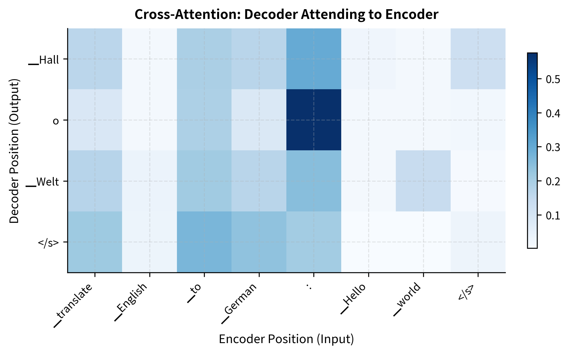
The masking in self-attention ensures the decoder can only see tokens it has already generated, maintaining the autoregressive property needed for text generation. Without this mask, the model could "cheat" during training by looking at future tokens, learning to copy rather than predict. Cross-attention allows each decoder position to attend to all encoder positions, integrating the input representation into the generation process. When generating a German translation, each German word can attend to all the English words, determining which parts of the source are most relevant for producing the current output token.
Information Flow
The complete forward pass proceeds through a two-stage process that first builds understanding and then produces output. First, input tokens are embedded and passed through all encoder layers. Each encoder layer refines the representations, with early layers capturing local syntactic patterns and deeper layers building more abstract semantic representations. The encoder's final hidden states, one vector per input token, become the "memory" that the decoder will reference throughout generation.
During generation, the decoder receives the previously generated tokens (or just a start token initially). These pass through self-attention layers with causal masking, allowing the model to consider what it has already said while deciding what to say next. Then cross-attention layers query the encoder memory, determining which parts of the input are relevant for generating the current token. The final decoder hidden state projects to vocabulary logits, and the highest-probability token becomes the next output. This process repeats, with each new token extending the decoder's self-attention context, until the model produces a stop token or reaches a maximum length.
T5-small uses 6 blocks in both the encoder and decoder. Let's examine a single encoder block to see its components:
The T5LayerSelfAttention handles self-attention with relative positions, while T5LayerFF implements the feed-forward network. Now let's compare with a decoder block:
The decoder adds a second attention layer (cross-attention) for attending to encoder outputs.
Relative Position Biases
Standard Transformers use absolute position embeddings. Each position in the sequence gets a fixed embedding vector added to the token embedding. T5 takes a different approach with relative position biases, which encode the distance between tokens rather than their absolute locations. This design decision reflects a better understanding of what position information the model actually needs.
Why Relative Positions?
Absolute positions have limitations that become apparent when you consider how humans process language. When reading the phrase "the big red ball," understanding that "big" and "red" both modify "ball" doesn't depend on whether this phrase appears at the beginning or middle of a paragraph. What matters is that these words are adjacent to each other. A model trained on sequences up to 512 tokens has never seen position 513, making generalization to longer sequences difficult with absolute positions. The embedding for position 513 simply doesn't exist, forcing awkward workarounds like position interpolation.
Relative positions encode the offset between the query and key positions in attention, capturing this linguistically meaningful notion of proximity. Whether two words appear at positions 10 and 15 or positions 100 and 105, they're "5 positions apart" in both cases. This translation invariance helps the model generalize across different sequence positions. A relationship learned between adjacent words at the beginning of training examples automatically transfers to adjacent words anywhere in any sequence.
The key insight is that position biases should modify attention scores directly. Rather than adding position information to token embeddings (which then influences attention indirectly through the learned query/key projections), T5 adds learned biases directly to the attention logits. In standard attention, the attention score between positions and becomes:
where:
- : the query vector at position
- : the key vector at position
- : the dimension of the key vectors (used for scaling)
- : the learned bias for relative position
Let's unpack what this formula tells us. The first term, , is the standard scaled dot-product attention score that measures content-based similarity between positions. This captures whether the semantic content at position wants to attend to the semantic content at position . The second term, , adds a position-based preference that depends only on how far apart the positions are, not where they sit in the sequence. A token might learn that it generally wants to attend strongly to the immediately preceding token (), regardless of content.
The bias term depends only on the distance between positions, not their absolute values. This allows the same position relationship to receive the same bias regardless of where it appears in the sequence. The model can learn, for example, that in English text, tokens often attend strongly to words 1-3 positions away (local syntactic patterns) while having weaker but still meaningful attention to more distant positions (long-range dependencies).
A learned scalar added to attention logits based on the distance between query and key positions. Unlike position embeddings added to token representations, position biases directly modulate attention weights.
T5's Position Bias Implementation
T5 uses a bucketed relative position scheme that balances expressiveness with parameter efficiency. Instead of learning a separate bias for every possible offset (which would require unbounded parameters as sequence length grows), T5 groups offsets into logarithmically spaced buckets. For a query at position and a key at position , the relative position is computed as:
where:
- : the relative position offset (positive when the key comes after the query, negative when before)
- : the position of the query token in the sequence
- : the position of the key token in the sequence
This offset is then mapped to a bucket index, and the model learns a bias value for each bucket. The bucketing strategy encodes an important insight: precise position differences matter more for nearby words than for distant ones. Whether a related word is exactly 57 or 62 positions away rarely changes its relevance, but whether it's 1 or 2 positions away often does.
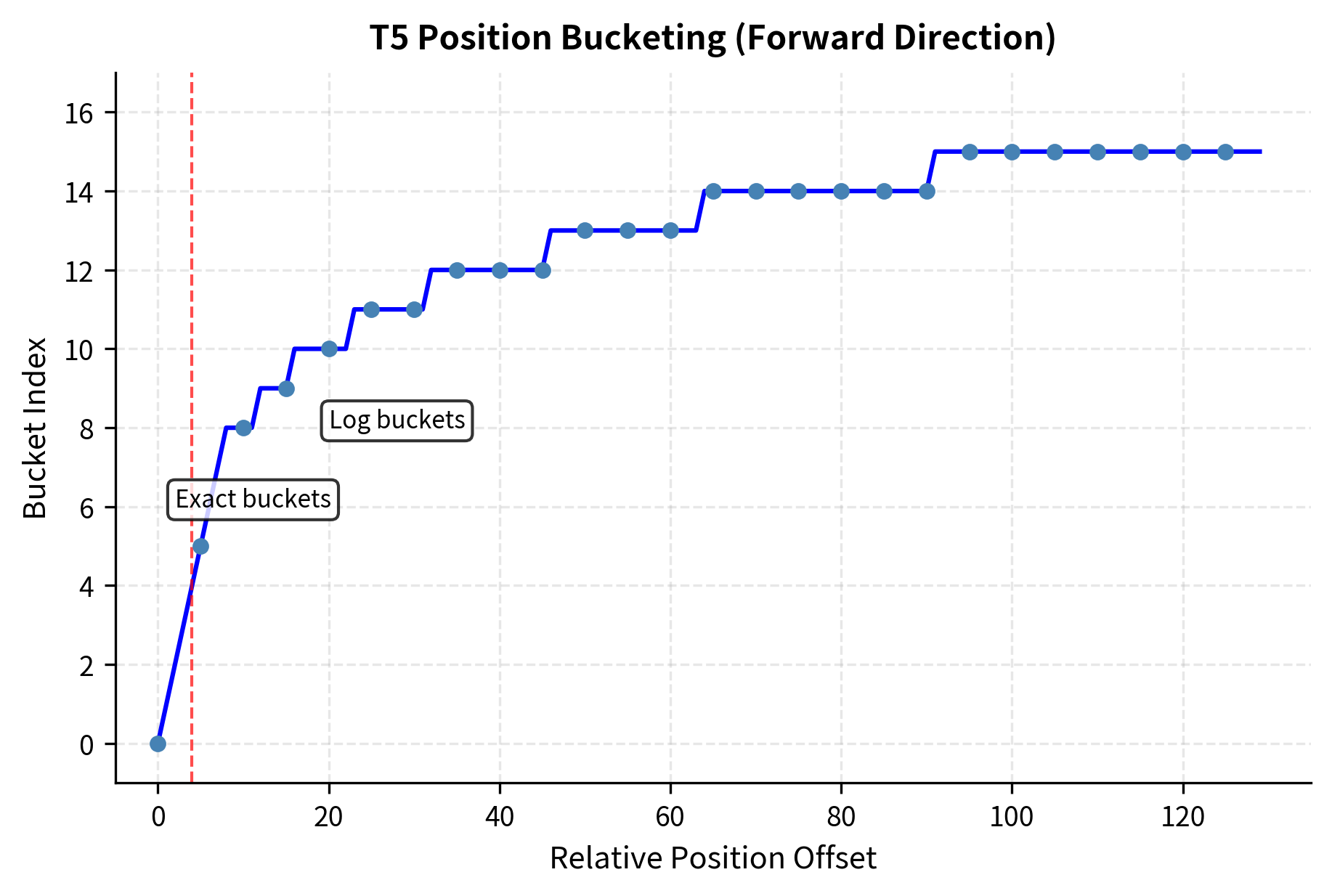
The bucketing works as follows:
- Compute the relative position: where is the query position and is the key position
- For small offsets, use exact values (each offset gets its own bucket)
- For larger offsets, use logarithmic bucketing (multiple offsets share a bucket)
- Look up the learned bias for that bucket
The logarithmic spacing means nearby positions (which often carry more grammatical signal) get fine-grained distinctions, while distant positions are grouped more coarsely. This keeps the parameter count manageable while still capturing useful position information. With 32 total buckets split between forward and backward directions, the model can represent a rich set of position relationships without requiring thousands of parameters per attention head.
For larger offsets, the bucket index is computed using logarithmic scaling:
where:
- : the final bucket index for this relative position
- : the number of buckets reserved for exact (small) offsets
- : the absolute value of the relative position offset
- : the maximum distance considered (default 128 in T5)
- : the number of buckets per direction (half the total buckets)
This formula deserves careful examination because it reveals the design philosophy behind T5's position encoding. The numerator measures how far beyond the exact-bucket threshold the offset reaches, on a logarithmic scale. Dividing by normalizes this to a value between 0 and 1 across the range of larger offsets. Multiplying by spreads these normalized values across the available buckets for large offsets. The floor operation ensures we get discrete bucket indices. Adding shifts the result into the correct range, after the buckets reserved for small exact offsets.
This formula maps offsets beyond into logarithmically-spaced buckets, ensuring that the distinction between positions 1 and 2 is preserved while positions 50 and 55 share the same bucket. The logarithmic spacing means bucket boundaries grow exponentially: perhaps buckets for offsets 1, 2, 3, 4, then 5-7, 8-15, 16-31, 32-63, and so on. This mirrors human perception of distance. We notice fine distinctions between nearby objects but group distant objects more coarsely.
Notice how small positive offsets (0, 1, 2) each get unique buckets, while larger offsets (20, 50, 100) start collapsing into shared buckets. Negative offsets (key before query) use a separate set of buckets, allowing the model to learn different biases for forward vs. backward attention. This asymmetry makes linguistic sense: attending to a word that came before ("I saw the") versus a word that comes after ("the dog ran") often serves different purposes, and the model can learn distinct patterns for each direction.
Visualizing Position Biases
Let's visualize the actual learned position biases from a trained T5 model:
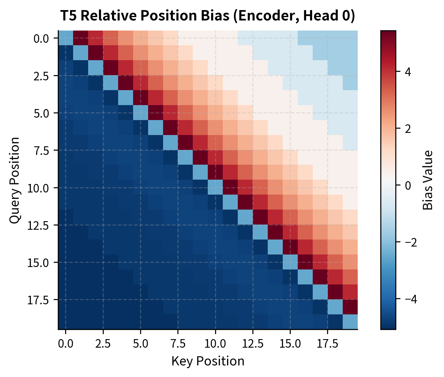
The bias pattern shows the model has learned to encourage attention to nearby positions (near the diagonal) while allowing more flexibility for distant positions. This structure emerges purely from training. The model discovers what relative position patterns help solve its pretraining objective.
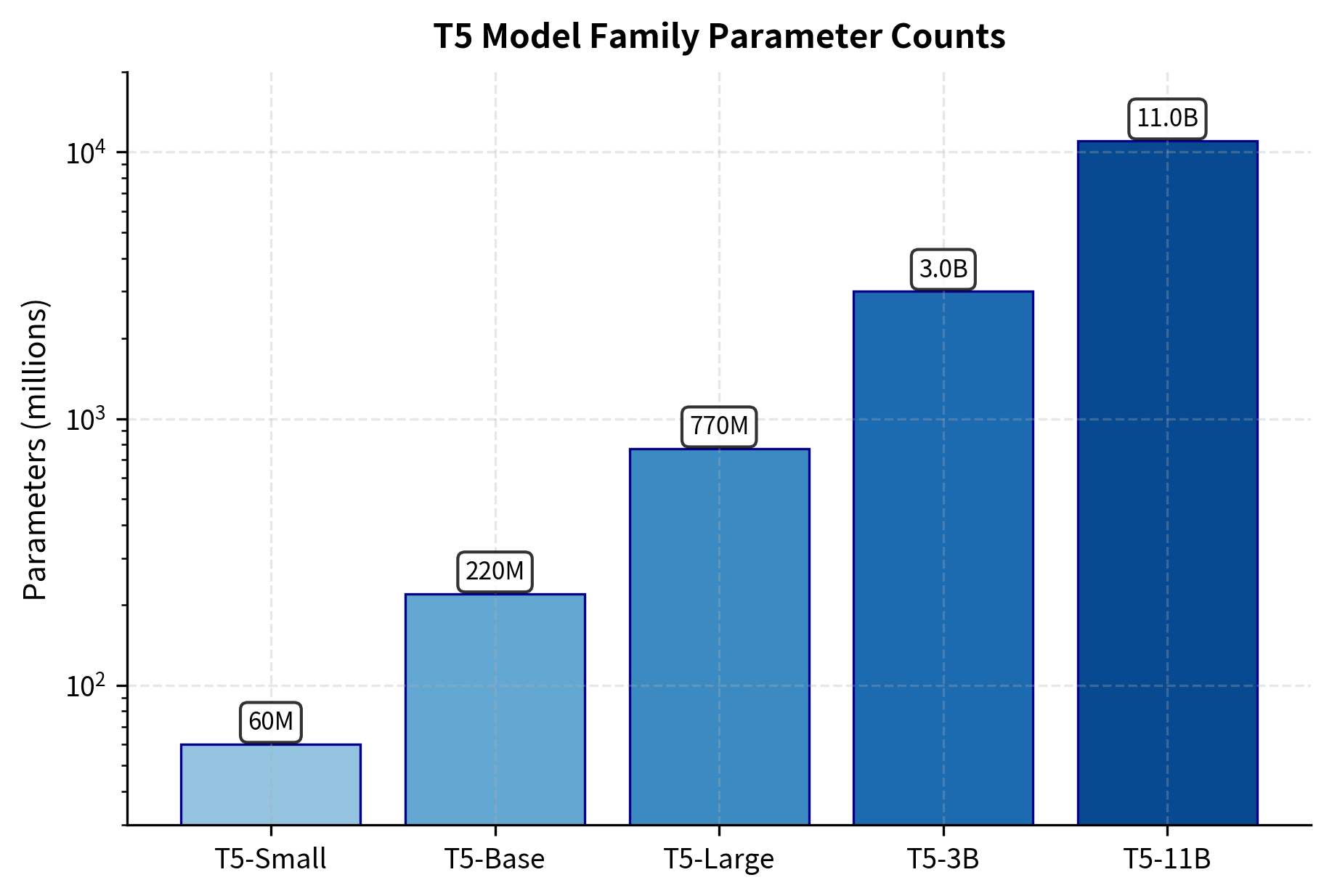
Model Sizes
T5 was released in five sizes, enabling researchers and practitioners to choose the right trade-off between capability and computational cost. Each size follows the same architecture but varies in depth, width, and total parameters.
| Model | Parameters | Layers | Hidden Size | Attention Heads | Feed-Forward Size |
|---|---|---|---|---|---|
| T5-Small | 60M | 6 | 512 | 8 | 2048 |
| T5-Base | 220M | 12 | 768 | 12 | 3072 |
| T5-Large | 770M | 24 | 1024 | 16 | 4096 |
| T5-3B | 3B | 24 | 1024 | 32 | 16384 |
| T5-11B | 11B | 24 | 1024 | 128 | 65536 |
Several patterns emerge from this scaling progression. Smaller models increase depth (more layers) as they grow, while the largest models hold depth constant and scale width instead. The feed-forward dimension grows proportionally larger at scale. The number of attention heads increases significantly for T5-3B and T5-11B, providing more specialized attention patterns.
The vocabulary size remains constant at 32,128 tokens across all sizes. This vocabulary was trained using SentencePiece on the C4 dataset, the same corpus used for pretraining.
Pretraining: Span Corruption
T5 uses a "span corruption" objective during pretraining, which the paper found more effective than alternatives like standard language modeling or BERT-style masked language modeling. This objective represents a good challenge that forces the model to develop robust language understanding.
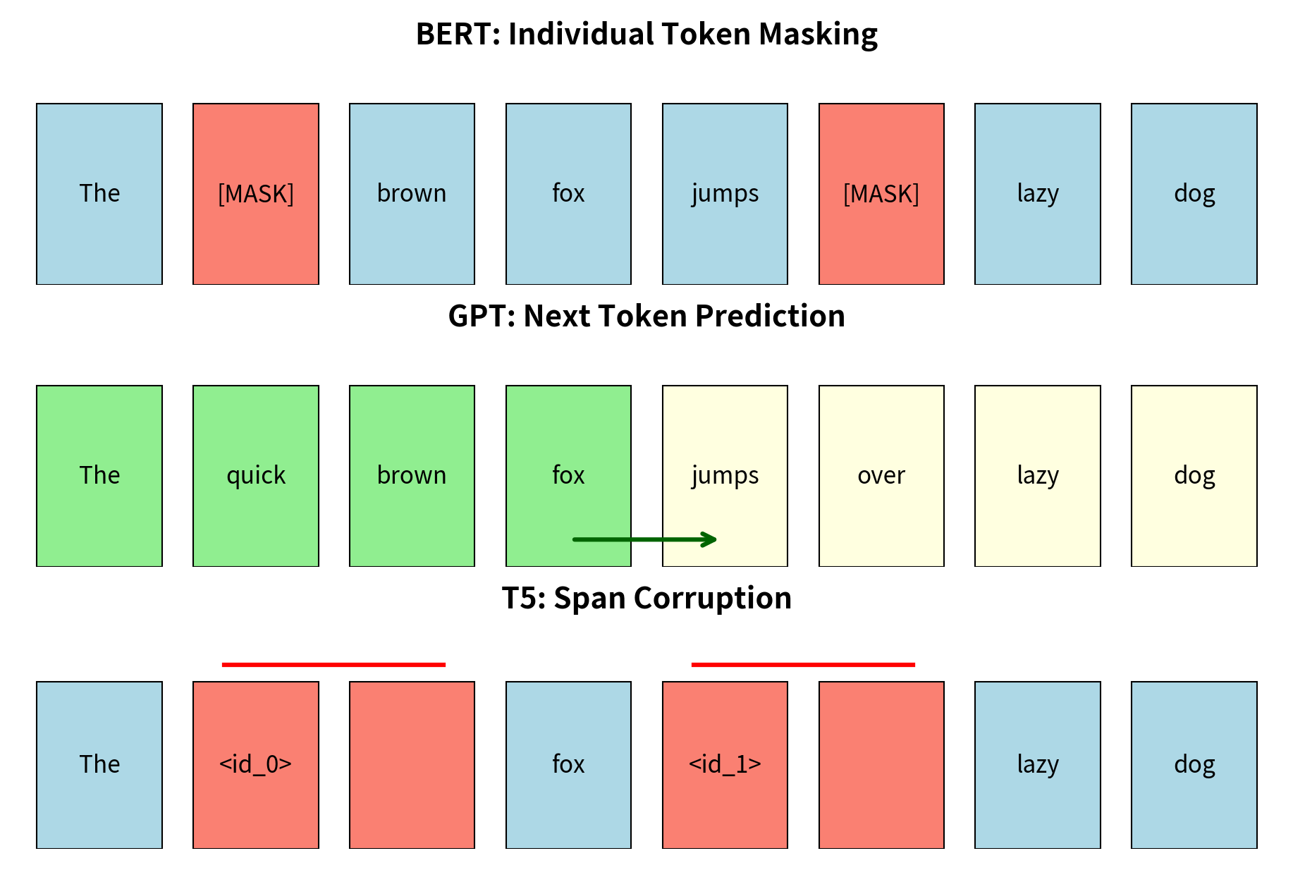
How Span Corruption Works
The objective corrupts the input by replacing contiguous spans of tokens with single sentinel tokens, then asks the model to reconstruct those spans. This approach differs from BERT's masked language modeling, which corrupts individual tokens, and from GPT's causal language modeling, which predicts the next token given previous context. Span corruption strikes a middle ground that encourages the model to understand broader context while still learning to generate coherent multi-token sequences.
Here's the process in detail:
- Sample span lengths from a distribution (mean length 3)
- Select 15% of tokens total to corrupt
- Replace each selected span with a unique sentinel token (
<extra_id_0>,<extra_id_1>, etc.) - Create targets that contain the sentinel followed by the original tokens
For example:
- Original:
The quick brown fox jumps over the lazy dog - Corrupted input:
The <extra_id_0> fox <extra_id_1> the lazy dog - Target:
<extra_id_0> quick brown <extra_id_1> jumps over
This approach forces the model to understand context deeply. It must determine what type of content belongs in each corrupted span based on surrounding words. Unlike next-token prediction (which only requires predicting one token at a time), span reconstruction requires understanding the complete context. When the model sees The <extra_id_0> fox jumps, it must recognize that the missing span should contain adjectives describing a fox, likely words like "quick brown" or "sly red." This requires understanding both syntax (adjectives precede nouns) and semantics (foxes have certain typical descriptions).
The use of contiguous spans rather than individual tokens adds another dimension of difficulty. The model cannot simply guess each missing token independently; it must generate a coherent sequence that fits grammatically and semantically as a unit. This trains the model for the kind of fluent generation required in downstream tasks like summarization and translation.
The sentinel tokens serve as placeholders in the input and anchors in the output, allowing the model to learn which span corresponds to which sentinel. This correspondence is crucial. By seeing <extra_id_0> in both input and output, the model learns that whatever follows <extra_id_0> in the target is what should fill the <extra_id_0> position in the input. The sentinel approach also makes the target sequence much shorter than the original input, improving training efficiency since the model only needs to generate the corrupted portions rather than reconstructing the entire input.
C4 Dataset
T5 was trained on the Colossal Clean Crawled Corpus (C4), a 750GB dataset derived from Common Crawl. The researchers applied extensive filtering to improve quality:
- Remove pages with fewer than 5 sentences
- Discard pages containing words from a blocklist
- Remove duplicate lines across the corpus
- Keep only English text (detected by language ID)
- Remove pages with too many repetitive patterns
This cleaning produced a dataset much larger than typical pretraining corpora at the time, enabling the scale experiments that T5 aimed to explore.
Working with T5
Let's use T5 for various tasks to see the text-to-text framework in action. We'll use T5-small for these examples to keep computational requirements modest.
Translation
Summarization
Examining Internal Representations
Let's look at how T5 processes input through its encoder:
Each layer produces a tensor of shape (batch_size, sequence_length, hidden_dim). The sequence has 11 tokens, and each token gets a 512-dimensional representation. Layer 0 is the embedding layer, and layers 1-6 are the transformer blocks.
Attention Pattern Visualization
Let's visualize how attention patterns differ between encoder and decoder:
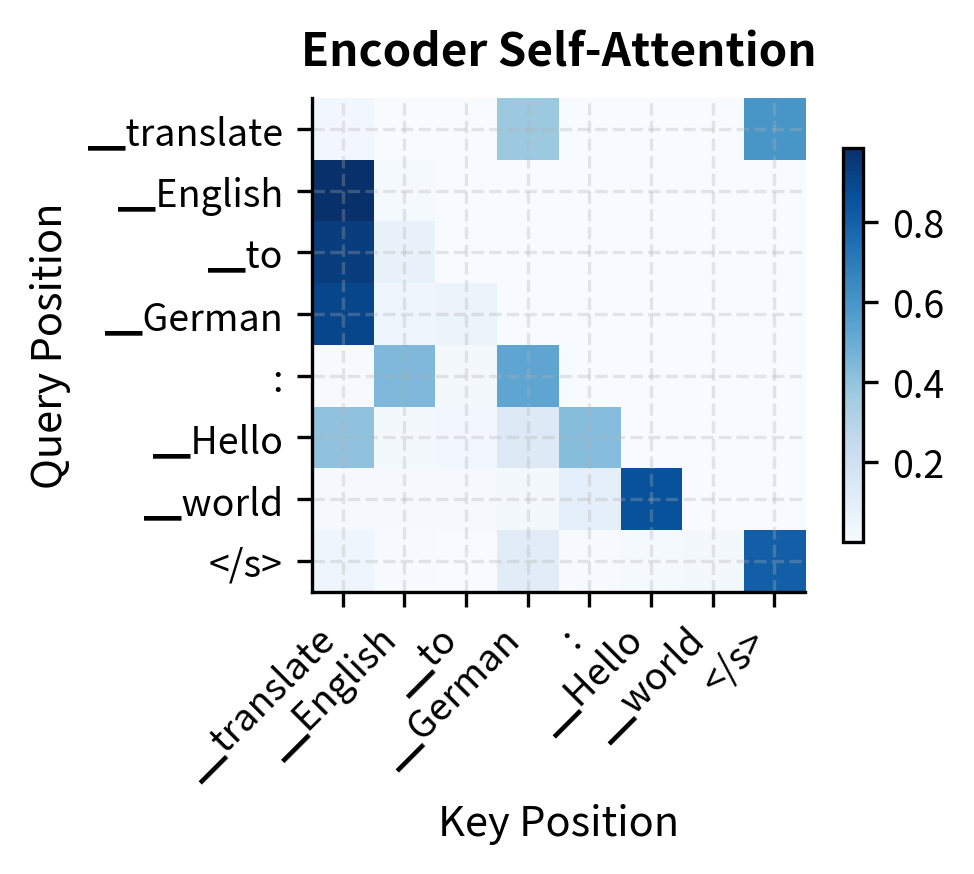
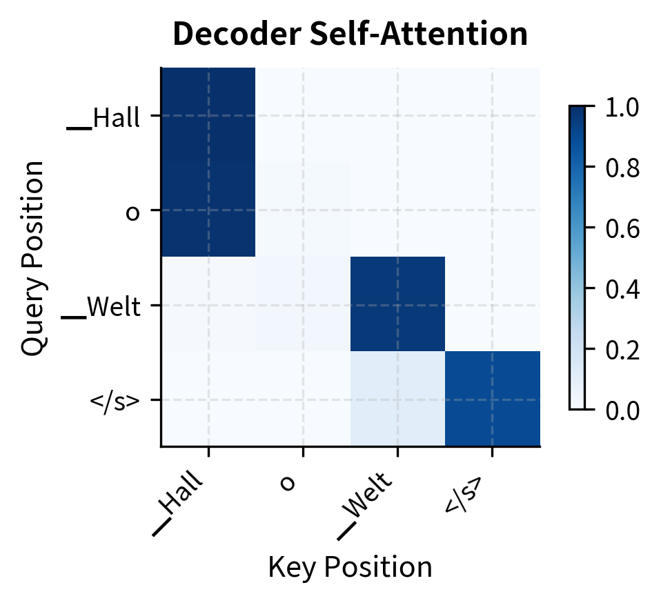
The encoder attention shows bidirectional patterns where tokens can attend freely to any position. The decoder attention shows the characteristic lower-triangular pattern from causal masking. Each token can only attend to itself and previous tokens, preventing information leakage from future positions during generation.
T5 Variants and Descendants
The T5 architecture inspired several important follow-up models that extended its capabilities:
-
Flan-T5 applied instruction tuning to T5, training on a diverse mixture of tasks phrased as natural language instructions. This dramatically improved zero-shot and few-shot performance, making the model more useful for novel tasks without task-specific fine-tuning.
-
mT5 (multilingual T5) extended pretraining to 101 languages using the mC4 dataset. This enabled cross-lingual transfer, where a model fine-tuned on English data can perform the same task in other languages.
-
LongT5 addressed T5's context length limitations by incorporating efficient attention mechanisms. Using transient global attention patterns, LongT5 handles documents up to 16,384 tokens while maintaining the encoder-decoder structure.
-
UL2 (Unified Language Learner) combined multiple pretraining objectives, including span corruption, prefix language modeling, and causal language modeling. This mixture of denoisers improved performance across diverse downstream tasks.
Limitations and Impact
T5's encoder-decoder architecture offers advantages for certain task types but introduces trade-offs compared to decoder-only alternatives. The bidirectional encoder excels when the full input must be processed before generating output. Summarization, translation, and question answering benefit from understanding the complete context first. However, this architecture requires separate encoder and decoder computations, increasing memory requirements compared to decoder-only models of similar parameter counts. For the same total parameters, a decoder-only model dedicates all capacity to a single transformer stack.
The text-to-text framework, while elegant, has practical limitations. Classification tasks produce output tokens that must be mapped back to discrete labels, adding a parsing step that can fail if the model generates unexpected text. For high-throughput classification in production, task-specific heads on BERT-style models often prove more efficient. Additionally, regression tasks require outputting numbers as text strings, which is less numerically precise than dedicated regression heads.
The impact of T5 on the field was significant. The systematic ablation study in the original paper influenced countless subsequent design decisions. Researchers could consult T5's experiments rather than re-running their own. The text-to-text framework demonstrated that unified architectures could match or exceed task-specific approaches, paving the way for general-purpose instruction-following models. T5's pretraining recipe, combining span corruption with massive-scale data, informed the development of models like PaLM and Flan-PaLM.
T5 also established that encoder-decoder architectures remained competitive even as decoder-only models (the GPT family) gained prominence. This architectural diversity has proven valuable. Encoder-decoder models continue to excel at translation and summarization, while decoder-only models dominate open-ended generation. Understanding both paradigms remains essential for practitioners choosing the right architecture for their specific application.
Summary
T5 unified NLP around a simple principle: treat every task as text-to-text generation. This framework eliminated the need for task-specific architectures, enabling a single model to handle translation, summarization, classification, and question answering through the same interface.
The architecture builds on the original Transformer's encoder-decoder design with key modifications. Pre-norm layer placement improves training stability. Relative position biases replace absolute position embeddings, encoding distances between tokens rather than their absolute locations. The bucketized position scheme keeps parameters bounded while capturing both fine-grained local and coarser global position information.
T5's five model sizes span from 60 million to 11 billion parameters, with systematic scaling that increases depth for smaller models and width for larger ones. The span corruption pretraining objective, replacing contiguous token spans with sentinels, proved more effective than alternatives like standard language modeling or masked language modeling.
The encoder-decoder structure particularly suits tasks requiring deep comprehension before generation. The encoder processes input bidirectionally, and the decoder generates output autoregressively while attending to encoded representations. This two-stage approach excels at translation and summarization, where understanding the full source is essential before producing the target.
T5's influence extended beyond its direct applications. The systematic ablation study guided subsequent architectural decisions. The text-to-text framework inspired instruction-tuning approaches that became central to modern language models. Variants like Flan-T5, mT5, and LongT5 extended its capabilities to instruction following, multilingual processing, and long-context understanding. By demonstrating that encoder-decoder models could compete with and sometimes exceed specialized architectures, T5 ensured this architectural family remained part of the practitioner's toolkit.

Comments