

Learn how T5 uses span corruption for pre-training. Covers sentinel tokens, geometric span sampling, the C4 corpus, and why span masking outperforms token masking.

This article is part of the free-to-read Language AI Handbook
Choose your expertise level to adjust how many terms are explained. Beginners see more tooltips, experts see fewer to maintain reading flow. Hover over underlined terms for instant definitions.
T5 Pre-training
T5, which stands for "Text-to-Text Transfer Transformer," introduced a unified approach to NLP that treats every task as converting input text to output text. While this text-to-text framework simplifies how we frame tasks, the model's remarkable capabilities stem largely from its innovative pre-training procedure. At the heart of T5's pre-training lies span corruption, a denoising objective that teaches the model to reconstruct corrupted portions of text.
Unlike BERT's approach of masking individual tokens, T5 corrupts contiguous spans of text and replaces them with single sentinel tokens. The model must then generate the missing content, producing the original spans in sequence. This design choice proves surprisingly effective: by predicting multiple consecutive tokens at once, the model learns richer contextual representations than single-token prediction allows.
The researchers at Google who developed T5 conducted an exhaustive empirical study, systematically testing dozens of architectural choices, pre-training objectives, and training configurations. The resulting paper, "Exploring the Limits of Transfer Learning with a Unified Text-to-Text Transformer," became a landmark reference for understanding what actually matters in training large language models. In this chapter, we'll examine the pre-training procedure that emerged from this exploration.
Span Corruption: The Core Objective
Span corruption transforms input text into a denoising task, fundamentally reshaping how the model learns to understand language. The core idea is straightforward: rather than asking a model to fill in individual blanks scattered throughout a sentence, we ask it to reconstruct entire missing phrases. This seemingly simple change has significant implications for what the model must learn.
Consider the difference between predicting a single missing word versus predicting a missing phrase. When filling in a single blank, a model can often succeed by identifying the grammatical category needed (noun, verb, adjective) and selecting a plausible word from that category. However, when an entire phrase is missing, the model must generate multiple words that not only fit the surrounding context but also cohere with each other. The phrase "large amounts" requires understanding that these two words naturally pair together, that they describe a quantity, and that they grammatically connect "require" to "of training data." This multi-token challenge forces the model to develop richer internal representations of language structure.
The procedure works in three distinct stages: selecting spans to corrupt, replacing them with sentinel tokens, and training the model to reconstruct the original spans. Each stage involves design decisions from extensive testing.
How Span Selection Works
The algorithm begins by deciding which tokens to corrupt, a process that must balance several competing concerns. We want enough corruption to provide meaningful training signal. If we corrupt too little, each training example teaches the model relatively little. However, we also want the task to remain solvable. If we corrupt too much, the model cannot reasonably infer what was removed. T5 uses a corruption rate of 15%, meaning roughly 15% of tokens in each sequence will be masked. This particular rate emerged from experiments as a good balance that provides strong learning signal while keeping the reconstruction task feasible.
However, rather than selecting tokens independently like BERT does, T5 groups consecutive tokens into spans. This grouping decision is not merely aesthetic. It fundamentally changes the nature of what the model learns. When BERT masks the word "fox" in "The quick brown fox jumps," the model learns that an animal noun fits this context. When T5 masks "brown fox" as a single span, the model must learn not only that an animal noun fits here, but also that adjective-noun pairs describing animals have particular patterns, that "brown" and "fox" co-occur naturally, and that the resulting phrase must connect smoothly with both "quick" before it and "jumps" after it.
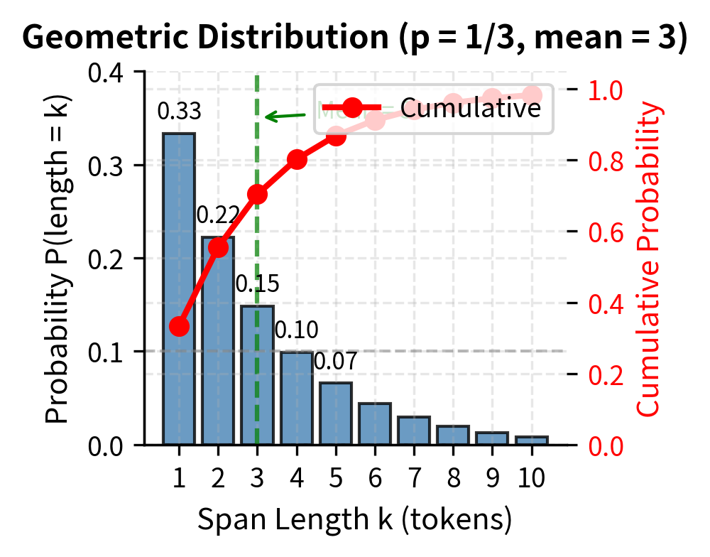
The span lengths follow a geometric distribution with a mean of 3 tokens. This means short spans are most common, but occasionally longer spans appear. Why a geometric distribution? This distribution has the useful property that span lengths are memoryless: given that a span has already reached length , the probability it continues for another token remains constant. This memoryless property simplifies the sampling procedure and ensures a natural spread of span lengths without complicated bookkeeping.
For a geometric distribution with mean , the probability of a span having exactly length is:
where:
- : the span length in tokens (must be at least 1)
- : the probability parameter of the geometric distribution, set to
- : the probability of "failing" to stop for the first tokens
- : the probability of "stopping" at exactly the -th token
To build intuition for this formula, imagine flipping a biased coin for each token in the span. The coin has probability of coming up "stop" and probability of coming up "continue." A span of length 1 occurs when we flip "stop" immediately on the first token, which happens with probability . A span of length 2 occurs when we flip "continue" on the first token (probability ) and then "stop" on the second (probability ), giving . A span of length 3 requires "continue, continue, stop," which is .
With , this gives us probabilities of approximately 33% for length 1, 22% for length 2, 15% for length 3, and so on. The distribution decays exponentially, ensuring that very long spans are rare but not impossible. This mix of span lengths exposes the model to a variety of reconstruction challenges: sometimes it must predict just a single word, sometimes a short phrase, and occasionally an extended expression.
Sentinel Tokens
A sentinel token is a special token that serves as a placeholder for corrupted spans. T5 uses a sequence of sentinel tokens (<extra_id_0>, <extra_id_1>, etc.) where each unique sentinel marks a different corrupted span in the input.
When T5 corrupts a span, it replaces the entire span with a single sentinel token, regardless of how many tokens the span contained. The first corrupted span becomes <extra_id_0>, the second becomes <extra_id_1>, and so forth. This compression is crucial: it means the corrupted input is significantly shorter than the original, making training more efficient.
The naming convention "extra_id" reflects that these tokens exist outside the normal vocabulary. They carry no inherent meaning and exist purely as markers. Think of them as numbered placeholders, similar to how a librarian might place numbered bookmarks where removed pages once sat. Each sentinel uniquely identifies which span was removed from that position, allowing the model to precisely reconstruct what belongs where.
This design choice has an elegant efficiency benefit. If a span contains four tokens and we replace it with a single sentinel, we've reduced the input length by three tokens. Across an entire sequence with multiple corrupted spans, these savings accumulate substantially. A 512-token input might shrink to 460 tokens after corruption, allowing the encoder to process more information per unit of computation. This efficiency gain compounds across millions of training examples.
The target sequence contains the sentinel tokens followed by the spans they replaced, in order. This creates a clear mapping between placeholders and their corresponding content. When the model sees <extra_id_0> in the encoder input, it knows that somewhere in the target sequence, <extra_id_0> will be followed by the exact tokens that belong in that position. The sentinel acts as both a placeholder in the input and a delimiter in the output.
The Input-Target Transformation
Let's trace through the complete transformation with a concrete example, examining each step to build intuition for how span corruption restructures text into a training signal. Consider this input sentence:
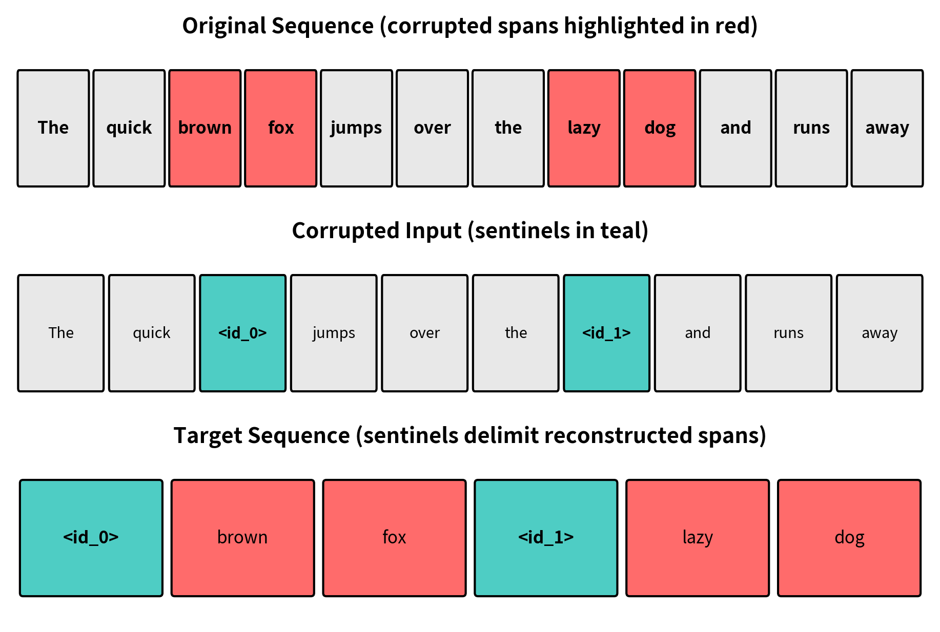
"The quick brown fox jumps over the lazy dog and runs away."
Suppose the span corruption procedure selects two spans: "brown fox" (positions 2-3) and "lazy dog" (positions 7-8). The transformation produces:
Corrupted Input:
"The quick
<extra_id_0>jumps over the<extra_id_1>and runs away."
Target Output:
"
<extra_id_0>brown fox<extra_id_1>lazy dog"
To understand why this format is so effective, let's examine what the model must learn to successfully complete this task. Looking at the corrupted input, the model sees that something is missing between "quick" and "jumps." This something immediately follows "quick" and is modified by it. The model must infer that this is likely an animal (because animals jump) and that "quick" suggests it's being described with adjectives. The surrounding context of a sentence about jumping and running further constrains the possibilities.
Notice several key properties of this transformation:
- The input is shorter than the original (sentinel tokens replace multi-token spans)
- Each sentinel appears exactly once in the input and once in the target
- The target contains only the corrupted spans, not the full original text
- Sentinels in the target act as delimiters separating the reconstructed spans
This design means the model predicts far fewer tokens than the original sequence length, making training computationally efficient while still requiring deep understanding of context. The model doesn't waste computation predicting tokens that weren't corrupted. It focuses its predictive capacity entirely on the challenging reconstruction task.
The one-to-one correspondence between sentinels in input and target creates an elegant bookkeeping system. During generation, when the model outputs <extra_id_0>, it signals that the following tokens should fill the position marked by <extra_id_0> in the input. When it outputs <extra_id_1>, it transitions to filling the next gap. This structure allows the decoder to generate all missing content in a single autoregressive pass, without needing special position-tracking mechanisms.
Mathematical Formulation
Having developed intuition for span corruption through examples, we can now formalize the objective mathematically. This formalization reveals the precise learning signal the model receives and connects span corruption to the broader family of sequence-to-sequence training objectives.
The span corruption objective can be formalized as follows. Given an input sequence , we:
- Sample span start positions and lengths according to the corruption parameters
- Replace each span with a unique sentinel token to produce
- Construct target by concatenating sentinels with their corresponding spans
The model is trained to maximize:
where:
- : the log-likelihood objective to maximize (equivalently, minimizing negative log-likelihood as the loss)
- : the target sequence containing sentinels and their corresponding original spans
- : the length of the target sequence
- : the -th token in the target sequence
- : all target tokens before position (the autoregressive context)
- : the input sequence with spans replaced by sentinel tokens
- : the model parameters (encoder and decoder weights)
- : the probability the model assigns to token given the corrupted input and previous target tokens
This formulation deserves careful unpacking. The summation runs over every token in the target sequence, meaning the model receives a learning signal for each prediction it makes. The conditioning on indicates that the encoder has processed the corrupted input and produced contextual representations that the decoder can attend to. The conditioning on reflects the autoregressive nature of the decoder: when predicting token , the model can see all previous target tokens it has generated.
This is the standard sequence-to-sequence cross-entropy loss, where the encoder processes the corrupted input and the decoder generates the target autoregressively. The encoder-decoder architecture is crucial here: the encoder builds rich bidirectional representations of the corrupted input (processing both left and right context simultaneously), while the decoder generates the target one token at a time, attending to both the encoder representations and its own previous outputs.
The strength of this formulation lies in its simplicity. Despite the somewhat complex corruption procedure, the training objective is identical to any other sequence-to-sequence task like machine translation. The model learns to generate the correct output sequence given the input sequence, and the span corruption simply defines what those input-output pairs look like during pre-training. This means the same architecture and training infrastructure developed for translation, summarization, and other seq2seq tasks applies directly to pre-training.
Why Span Corruption Outperforms Token Masking
The T5 paper compared span corruption against several alternatives, including BERT-style token masking. Span corruption consistently performed better for several reasons, each stemming from fundamental differences in what the model must learn.
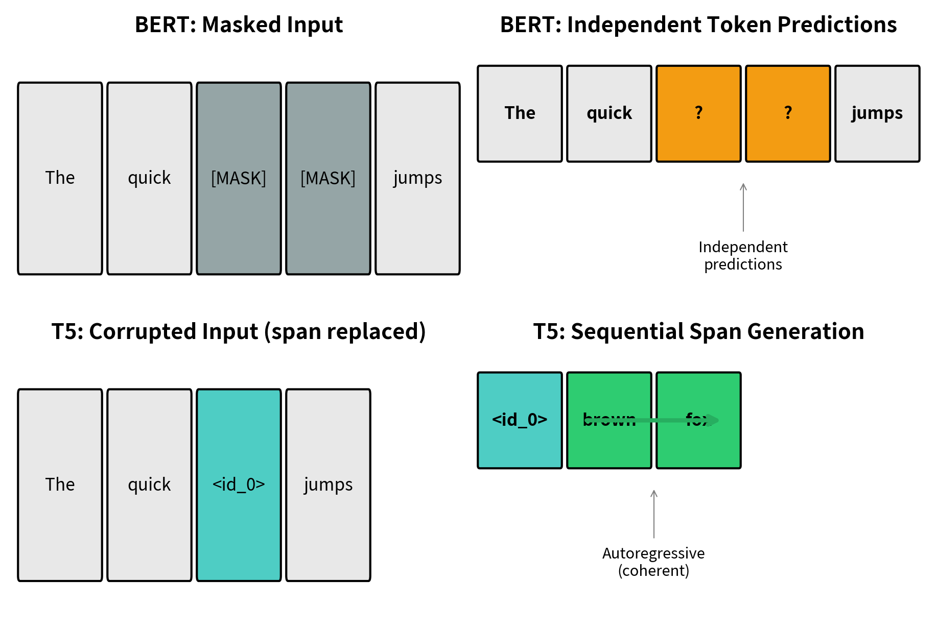
When BERT masks tokens, each masked position is predicted independently using bidirectional context. The model produces a probability distribution over the vocabulary for each masked position, but these predictions don't need to cohere with each other. If "The [MASK] [MASK] jumps" has two masked positions, BERT predicts each independently. It might assign high probability to "brown" for the first position and high probability to "cat" for the second, even though "brown cat" would be unusual in context while "brown fox" would be natural.
Span corruption eliminates this incoherence problem entirely. When the decoder generates "brown fox" to fill a single span, it produces "fox" after having already committed to "brown." The autoregressive generation ensures that multi-token predictions are internally consistent. The model learns not just which words fit each position, but which word sequences form natural phrases.
The key advantages of span corruption include:
- Richer predictions: Generating multiple consecutive tokens requires modeling local coherence, not just fill-in-the-blank vocabulary matching
- Computational efficiency: Replacing spans with single sentinels shortens inputs, allowing larger batch sizes or longer sequences
- Better calibration: The model learns to generate varying-length outputs, preparing it for downstream generation tasks
The corruption rate of 15% with mean span length 3 emerged from extensive testing as an effective balance. Higher corruption rates provide more training signal per example but can make the task too difficult. Lower rates are easier but provide less learning signal. The mean span length of 3 ensures a good mix of single-token, short-phrase, and occasional longer-phrase predictions, exposing the model to reconstruction challenges at multiple scales.
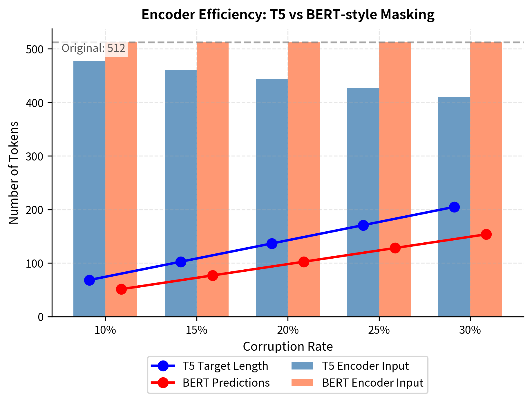
The efficiency benefit is particularly important. Consider a 512-token input with 15% corruption (approximately 77 tokens masked). With BERT-style masking, the input remains 512 tokens, and the model predicts 77 tokens. With T5-style span corruption, assuming approximately 26 spans (77 tokens ÷ 3 mean length), the corrupted input shrinks to roughly 461 tokens (512 - 77 + 26). The encoder processes fewer tokens while the decoder still predicts the same 77 tokens of content. This efficiency compounds across the billions of training examples in pre-training.
Worked Example: Step-by-Step Corruption
Let's walk through the span corruption algorithm in detail, tracing each step to solidify understanding. This worked example will make the abstract procedure concrete, showing exactly how a sentence transforms into a training example. We'll use a simple sentence and trace each step.
Original text: "Machine learning models require large amounts of training data."
Step 1: Tokenization
Before any corruption occurs, the text must be converted to tokens. This step matters because corruption operates at the token level, not the word level. T5 uses SentencePiece tokenization, which might split words into subwords, but for this example we'll use word-level tokenization for clarity.
After tokenization (using T5's SentencePiece tokenizer), we might get:
| Position | 0 | 1 | 2 | 3 | 4 | 5 | 6 | 7 | 8 | 9 |
|---|---|---|---|---|---|---|---|---|---|---|
| Token | Machine | learning | models | require | large | amounts | of | training | data | . |
Each position in this sequence is now a candidate for inclusion in a corrupted span. The algorithm will select some of these positions to mask, group them into spans, and replace those spans with sentinels.
Step 2: Determine corruption budget
With 10 tokens and a 15% corruption rate, we aim to corrupt approximately 1.5 tokens. In practice, the algorithm samples span lengths that sum close to this target. The 15% rate is a target, not an exact requirement. Individual examples may vary slightly while the average across many examples approaches 15%.
In this short example, the low corruption budget means we'll likely corrupt just one short span. Longer sequences would have multiple spans, creating more complex reconstruction tasks.
Step 3: Sample span positions and lengths
The algorithm might sample one span of length 2 starting at position 4. This corrupts "large amounts." The choice of which positions to corrupt is random, ensuring the model sees varied examples. Some training examples might corrupt the beginning of sentences, others the middle or end, and still others might have multiple scattered spans.
Step 4: Apply corruption
Replace positions 4-5 with <extra_id_0>:
| Position | 0 | 1 | 2 | 3 | 4 | 5 | 6 | 7 | 8 |
|---|---|---|---|---|---|---|---|---|---|
| Token | Machine | learning | models | require | <extra_id_0> | of | training | data | . |
Notice that the corrupted sequence is now 9 tokens instead of 10. The two-token span "large amounts" has been replaced by the single token <extra_id_0>, achieving the compression that makes span corruption efficient. The sentinel serves as a placeholder that unambiguously marks where content was removed.
Step 5: Construct target
The target becomes: <extra_id_0> large amounts
The target sequence begins with the sentinel token, followed by the content of the span that sentinel replaced. If there were multiple spans, the target would contain multiple sentinel-content pairs in order: <extra_id_0> first span content <extra_id_1> second span content, and so forth.
Final result:
- Input: "Machine learning models require
<extra_id_0>of training data." - Target: "
<extra_id_0>large amounts"
The model learns that given the context of "models require ___ of training data," the missing span should be "large amounts." To succeed at this task, the model must understand that "require" takes a noun phrase object, that "of training data" suggests the object describes a quantity, and that "large amounts" is a natural phrase that satisfies these constraints. This single example teaches vocabulary, grammar, phrase structure, and world knowledge simultaneously.
Code Implementation
Let's implement span corruption from scratch to understand the mechanics, then see how to use the actual T5 tokenizer. Building the algorithm ourselves reveals the design decisions that make span corruption work, while the practical implementation shows how these ideas integrate with real NLP pipelines.
Building Span Corruption
We'll start by implementing the core span selection logic. This function samples span lengths from a geometric distribution, ensuring we corrupt approximately the target fraction of tokens while respecting the random nature of span lengths:
With 100 tokens, we generated 5 spans of varying lengths that together corrupt 15% of the sequence. Notice how the span lengths vary. We got a mix of short and medium-length spans, exactly what the geometric distribution produces. Now let's implement the full corruption procedure, which must not only sample span lengths but also place them in the sequence without overlapping:
The implementation carefully handles span placement to avoid overlaps. It tracks which positions have already been claimed by earlier spans and only places new spans in the remaining available positions. The final sorting step ensures sentinels appear in reading order, matching T5's expected format.
Let's test our implementation on a real sentence:
The corrupted input is shorter than the original because multi-token spans are replaced by single sentinel tokens. The target contains only the sentinels and their corresponding spans, making it much shorter than the full reconstruction target used in BERT-style approaches. This efficiency, with shorter inputs and focused targets, compounds across millions of training examples to significantly reduce computational costs.
Using the T5 Tokenizer
In practice, you'll use the Hugging Face transformers library which handles tokenization and provides pre-trained models. The library's tokenizer includes all the sentinel tokens and correctly handles the subword tokenization that T5 expects:
T5's tokenizer includes 100 sentinel tokens by default, allowing for up to 100 separate spans to be corrupted in a single example. The token IDs are at the end of the vocabulary, keeping them separate from regular text tokens. This separation is intentional: sentinel tokens should never appear in normal text, so placing them at vocabulary boundaries helps prevent accidental collisions.
Examining Real T5 Tokenization
Let's see how T5's SentencePiece tokenizer handles our example text. SentencePiece tokenization can split words into subwords, which affects how span corruption operates at a fine-grained level:
T5 uses SentencePiece tokenization, which may split words into subword units. The underscore character (▁) indicates the start of a new word in the original text. This subword approach allows T5 to handle rare words and morphological variations gracefully. Even words never seen during training can be represented as combinations of known subwords.
T5 Pre-training Data: The C4 Corpus
T5 was pre-trained on the Colossal Clean Crawled Corpus (C4), a massive dataset created specifically for this research. Understanding C4 helps explain T5's capabilities and limitations.
C4 Construction
C4 was derived from Common Crawl, a publicly available web scrape. The researchers applied aggressive filtering to clean the data:
- Language filtering: Only English text was retained, using a language detection model
- Quality heuristics: Pages were removed if they contained fewer than 5 sentences, had sentences shorter than 3 words, or contained offensive words from a blocklist
- Deduplication: Exact duplicate paragraphs were removed across the entire corpus
- JavaScript/boilerplate removal: Common web artifacts like "Terms of Service" and cookie notices were filtered out
The resulting dataset contains approximately 750 GB of clean text, roughly 156 billion tokens. This scale was unprecedented at the time and enabled training much larger models than previous work.
Quality vs. Quantity Tradeoffs
The T5 paper experimented with different levels of filtering. More aggressive filtering produced higher-quality text but reduced dataset size. The researchers found that:
- Light filtering produced worse downstream performance despite more data
- Heavy filtering (C4) struck a good balance between quality and quantity
- Extremely aggressive filtering reduced the dataset too much, hurting performance
This finding influenced subsequent work on LLM pre-training, emphasizing that data quality often matters more than raw quantity.
T5 Training Scale
The T5 paper introduced models at five different scales, enabling systematic study of how performance varies with model size.
Model Variants
T5 was released in five sizes:
| Model | Parameters | Encoder Layers | Decoder Layers | Hidden Size | Attention Heads |
|---|---|---|---|---|---|
| T5-Small | 60M | 6 | 6 | 512 | 8 |
| T5-Base | 220M | 12 | 12 | 768 | 12 |
| T5-Large | 770M | 24 | 24 | 1024 | 16 |
| T5-3B | 3B | 24 | 24 | 1024 | 32 |
| T5-11B | 11B | 24 | 24 | 1024 | 128 |
As shown in Table t5-variants, the largest model (T5-11B) achieved state-of-the-art results on numerous benchmarks at the time of release. The size progression allowed researchers to study scaling laws and helped establish that larger models consistently perform better when trained appropriately.
Training Configuration
T5 models were trained with the following key hyperparameters:
- Sequence length: 512 tokens for both encoder and decoder
- Batch size: 128 sequences (65,536 tokens per batch for T5-Base)
- Training steps: 1 million steps for the base configuration
- Optimizer: Adafactor, a memory-efficient variant of Adam
- Learning rate: Inverse square root decay schedule
The total compute for T5-11B was substantial, requiring multiple TPU pods running for weeks. This level of investment established a new baseline for what's possible with sufficient resources.
Effective Training Tokens
With 1 million training steps and batch size 128, the model sees:
With 512 tokens per sequence:
This means T5 was trained for less than one epoch over C4, seeing each example on average less than once. This is common in large-scale pre-training: the dataset is so large that even partial coverage provides sufficient training signal.
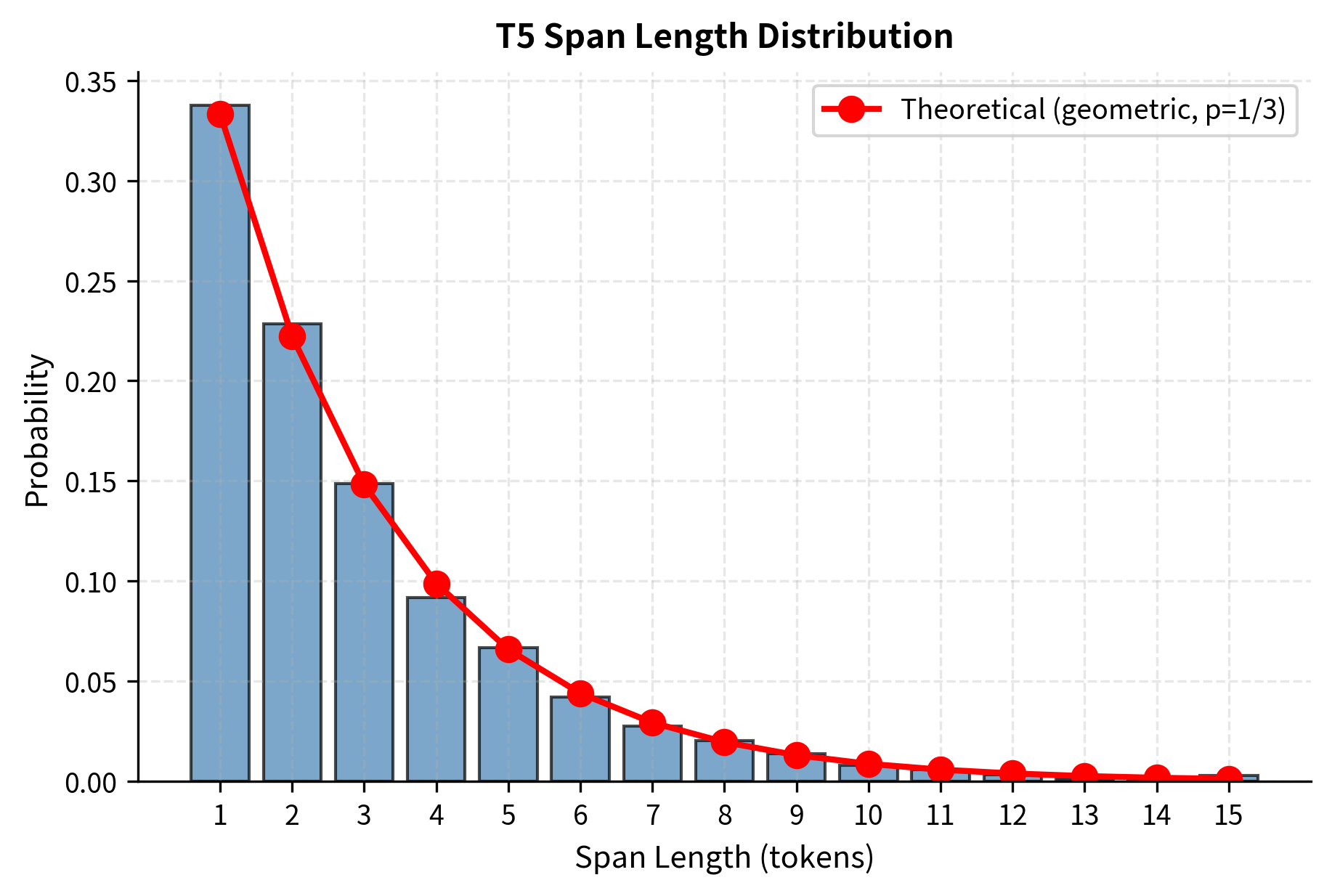
Visualizing Span Corruption Statistics
Let's examine the distribution of span lengths and corruption patterns:
The empirical distribution closely matches the theoretical geometric distribution. About one-third of spans contain just a single token, making span corruption somewhat similar to token-level masking in many cases. However, the longer spans provide valuable training signal for learning longer-range dependencies.
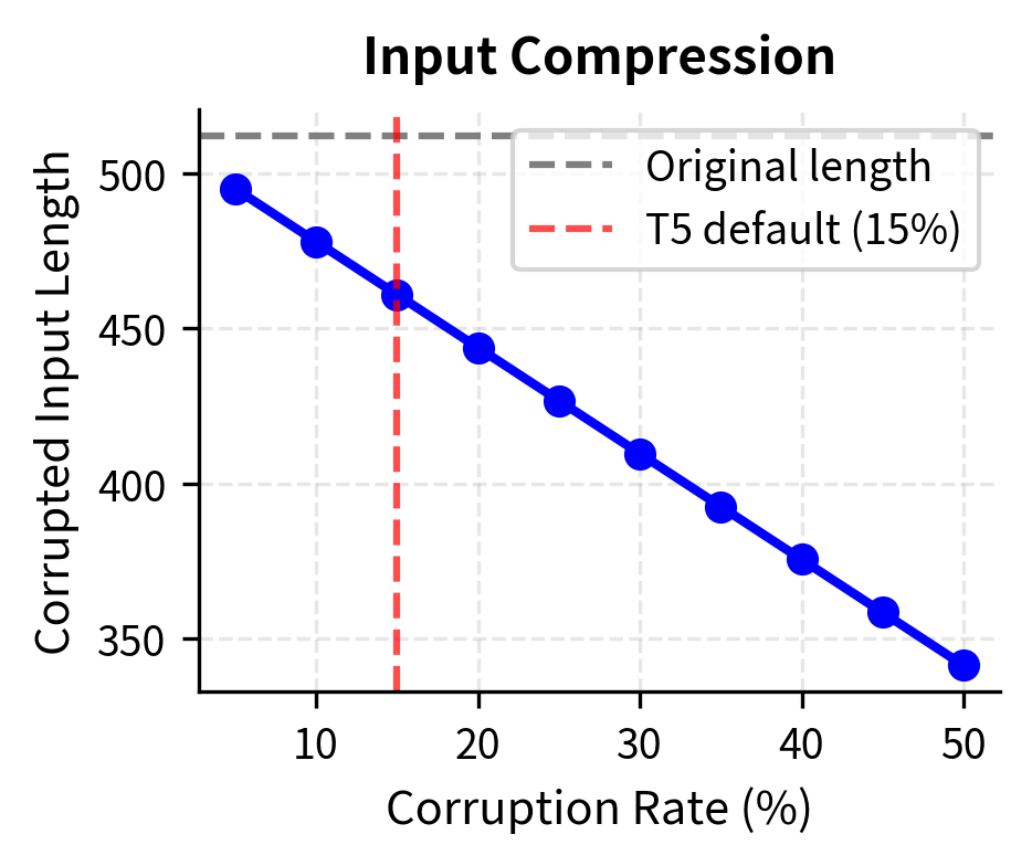
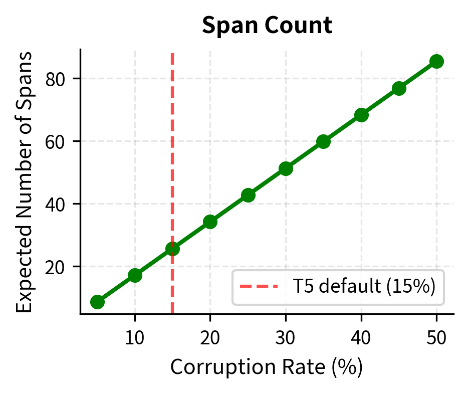
At T5's default 15% corruption rate with mean span length 3, we expect about 25 spans in a 512-token sequence. The input length shrinks to roughly 460 tokens because each multi-token span is replaced by a single sentinel.
Limitations and Impact
T5's pre-training approach, while innovative and effective, has several important limitations and requirements that shaped its adoption and influence on the field.
Computational Requirements
T5's pre-training demands significant resources. Training T5-11B required TPU pods running for extended periods, placing such models out of reach for most researchers. Even inference with the largest models requires specialized hardware. This computational barrier led to a focus on smaller variants (T5-Small, T5-Base) for practical applications.
The span corruption objective itself is efficient, producing targets shorter than the original input. However, the encoder-decoder architecture processes sequences twice (once in the encoder, once in the decoder), making T5 less efficient than decoder-only models for pure generation tasks.
Data Limitations
C4's English-only focus means T5 underperforms on non-English tasks without additional multilingual training. The web-crawled data also contains biases present in internet text, and the quality filtering may have inadvertently removed certain types of legitimate content. Later work addressed some of these issues with mT5 (multilingual T5) and updated versions of the C4 corpus.
What T5 Unlocked
Despite these limitations, T5 had substantial impact on the field:
The text-to-text framework demonstrated that diverse NLP tasks could be unified under a single paradigm. Rather than designing task-specific architectures, researchers could cast any problem as text generation. This simplified both training and deployment, as a single model could handle classification, generation, question answering, and translation.
The systematic empirical study in the T5 paper established methodological standards for LLM research. By testing many design choices in a controlled setting, the authors provided evidence-based guidance that influenced subsequent work. Findings about data quality, model scaling, and training objectives became foundational knowledge.
T5 also demonstrated the continued relevance of encoder-decoder architectures. While GPT-style decoder-only models dominated certain applications, T5 showed that encoders provide advantages for tasks requiring deep understanding of input context before generating output.
Comparison with Other Approaches
Span corruption occupies a middle ground between BERT's masked language modeling and GPT's causal language modeling:
| Approach | Input Processing | Target | Best For |
|---|---|---|---|
| BERT MLM | Bidirectional | Single masked tokens | Classification, NLU |
| T5 Span Corruption | Bidirectional | Corrupted spans | Conditional generation |
| GPT CLM | Causal (left-to-right) | Next token | Open-ended generation |
As shown in Table pretraining-comparison, T5's approach excels when the task has clear input-output structure, such as translation, summarization, or question answering. For open-ended generation without explicit conditioning, decoder-only models tend to be more natural fits.
Summary
T5 pre-training centers on span corruption, a denoising objective that teaches the model to reconstruct corrupted portions of text. The key innovations include:
-
Span-level masking: Rather than individual tokens, T5 masks contiguous spans of text with an average length of 3 tokens. This provides richer training signal than single-token prediction.
-
Sentinel tokens: Each corrupted span is replaced by a unique sentinel token (
<extra_id_0>,<extra_id_1>, etc.), creating a compact input representation. The model learns to map these placeholders back to their original content. -
Efficient targets: The target sequence contains only the corrupted spans, not the full original text. This makes training more computationally efficient while still requiring comprehensive understanding of context.
-
The C4 corpus: T5 introduced a carefully filtered 750 GB dataset derived from Common Crawl, demonstrating that data quality significantly impacts downstream performance.
-
Scale studies: With models ranging from 60 million to 11 billion parameters, T5 established clear scaling relationships and provided the community with models at various resource requirements.
The span corruption objective, combined with the text-to-text framework, produced models that achieved state-of-the-art results across diverse benchmarks. While subsequent decoder-only models have dominated headlines, T5's encoder-decoder architecture and pre-training approach remain highly effective for tasks with clear input-output structure, continuing to influence modern NLP systems.
Quiz
Ready to test your understanding? Take this quick quiz to reinforce what you've learned about T5's span corruption pre-training objective.

Comments