

Learn BART's denoising pre-training approach including text infilling, token masking, sentence permutation, and how corruption schemes enable generation.

This article is part of the free-to-read Language AI Handbook
Choose your expertise level to adjust how many terms are explained. Beginners see more tooltips, experts see fewer to maintain reading flow. Hover over underlined terms for instant definitions.
BART Pre-training
In the previous chapter, we explored BART's bidirectional encoder and autoregressive decoder architecture. Now we turn to what makes BART distinctive: its pre-training strategy. While BERT uses masked language modeling and GPT uses causal language modeling, BART takes a fundamentally different approach by framing pre-training as denoising autoencoding. The model learns to reconstruct original text from deliberately corrupted inputs, and the specific corruption schemes determine what linguistic knowledge BART acquires.
What makes BART's approach powerful is its flexibility. Rather than committing to a single corruption strategy, the researchers experimented with five different noising functions and their combinations. Each corruption type forces the model to learn different aspects of language, from local token patterns to document-level structure. This chapter examines each noising scheme in detail, explores why certain combinations work better than others, and implements the key corruption functions.
The Denoising Framework
BART's pre-training objective is simple: given a corrupted document , reconstruct the original document . This turns the abstract problem of "learning language" into a concrete task: undo the corruption and recover the original text. The approach works because the objective creates rich learning signals based on how we corrupt the input.
The model minimizes negative log-likelihood loss:
where:
- : the loss function to minimize (negative log-likelihood)
- : the original uncorrupted document
- : the number of tokens in the original document
- : the -th token of the original document
- : all tokens before position (the decoder's previous outputs)
- : the corrupted version of the document (encoder input)
- : the probability the model assigns to the correct token
Consider what happens at each decoding step. The model uses two information sources: the corrupted input processed by the encoder, and the previously generated tokens . With these, the model predicts the probability distribution over all possible next tokens. We measure how much probability mass it assigns to the correct token . The logarithm converts multiplicative probabilities into additive quantities. The negative sign changes our goal from maximizing likelihood to minimizing loss, which is standard in optimization.
This is cross-entropy loss over the original tokens, conditioned on both the previously generated tokens and the corrupted input. The encoder processes , and the decoder generates token by token. The summation over all tokens means we get a training signal at every position in the sequence, not just corrupted ones. This dense supervision distinguishes BART from BERT, which only computes loss at masked positions.
A model that learns to reconstruct clean data from corrupted versions. The corruption process is called "noising," and the reconstruction process is "denoising." The model learns robust representations by being forced to fill in missing or corrupted information.
The key design choice is selecting the noising function that transforms into . This function determines what the model learns during pre-training. Different noising functions create different learning signals. Some emphasize local word relationships, others stress document structure, and some require the model to infer the length of missing content. If corruption is too easy to reverse, the model learns little because it can trivially recover the original without developing strong linguistic understanding. If corruption is too difficult or destroys too much structure, the model cannot learn meaningful patterns because there's insufficient signal remaining to guide reconstruction. BART's innovation was systematically exploring this design space to identify corruptions that hit the sweet spot: challenging enough to force learning but structured enough to permit it.
Unlike BERT, which only predicts masked tokens, BART's decoder must generate the entire original sequence. This architectural choice affects training. The model receives a training signal for every token position, not just corrupted ones. Even "easy" positions where the input was not corrupted contribute to learning. The decoder must copy these tokens and position them correctly within the output sequence. Unlike T5, which uses a specific span corruption scheme with sentinel tokens, BART explores a broader range of corruption strategies and reconstructs exact original text rather than just the corrupted spans. This full-sequence reconstruction teaches the model to blend generated content with copied content, a skill relevant to tasks like summarization where the output combines novel phrases with material drawn from the source.
Token Masking
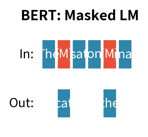
Token masking is the most familiar corruption scheme, directly inherited from BERT's masked language modeling objective. Random tokens are replaced with a special [MASK] token, and the model must predict the original tokens. This approach has proven remarkably effective for learning contextual word representations, and BART includes it as one of its corruption options to benefit from these established strengths.
How It Works
Given a sequence of tokens, we mask each token independently with probability (typically 15%, following BERT). The independence means that each token's fate is determined by its own random draw, without consideration of neighboring tokens:
where:
- : the -th token in the corrupted sequence
- : the -th token in the original sequence
- : the masking probability (typically 0.15)
- : a special token indicating a masked position
This piecewise definition captures a simple stochastic process: for each position , flip a biased coin that lands on "mask" with probability and "keep" with probability . The resulting corrupted sequence has the same length as the original, with [MASK] tokens scattered throughout. The specific positions vary each time we corrupt the same document, providing varied training examples from identical source text.
For example, the sentence "The quick brown fox jumps over the lazy dog" might become "The [MASK] brown fox [MASK] over the lazy [MASK]". Notice that the structure remains intact. We can still see that something describes "brown," that an action connects "fox" to "over," and that some modifier precedes "dog." These structural clues are precisely what the model must learn to exploit.
What the Model Learns
Token masking teaches the model to use bidirectional context for word prediction. To predict "quick," the encoder must understand that something describing "fox" fits between "The" and "brown." The model learns that adjectives typically precede the nouns they modify, that certain adjectives co-occur (quick and brown both describe animals in motion), and that syntactic patterns constrain what words can appear where. This develops strong contextual word representations, the same capability that makes BERT effective for classification and extraction tasks where understanding word meaning in context matters most.
However, token masking has limitations that become apparent when we consider generation tasks. The corruption is always one-to-one: one mask corresponds to exactly one original token. This rigid correspondence means the model never learns to handle situations where the number of output tokens differs from the number of input tokens, an important skill for generation tasks. When summarizing, the model must compress many input tokens into fewer output tokens. When elaborating or explaining, it must expand. Token masking provides no training signal for these variable-length transformations.
With a 30% masking rate (higher than typical for visibility), several tokens are replaced with the [MASK] placeholder. The decoder must generate all original tokens, but the key learning signal comes from correctly predicting the masked positions. The output shows which token indices were masked, allowing us to verify the corruption is working as expected.
Token Deletion
Token deletion takes masking one step further: instead of replacing tokens with a placeholder, we remove them entirely. This seemingly small change has significant implications for what the model must learn. Where masking leaves behind a marker saying "something was here," deletion removes all evidence of the token's existence, forcing the model to infer not just what is missing but also where the gaps are.
How It Works
Random tokens are deleted from the sequence with probability :
where:
- : the corrupted sequence (a subset of the original tokens)
- : the -th token in the original sequence
- : a random value drawn independently for each token
- : each is drawn uniformly from the interval
- : the deletion probability
The notation uses set-builder notation to express "keep only those tokens where the random draw exceeds ." Since each is uniformly distributed between 0 and 1, the probability that is exactly , meaning each token survives with probability . The corrupted sequence is shorter than the original (its expected length is times the original length), and crucially, there's no marker indicating where deletions occurred. The tokens that remain simply adjoin each other, closing the gaps left by deleted content.
For example, "The quick brown fox jumps over the lazy dog" might become "The brown fox over lazy dog" with "quick," "jumps," "the," and possibly other tokens deleted. The resulting sequence reads almost grammatically but contains subtle errors.missing descriptors, absent verbs, dropped articles.that reveal the corruption.
What the Model Learns
Token deletion forces the model to solve two problems simultaneously, which creates a richer learning signal than masking alone:
- Detection: Where were tokens deleted? Without mask tokens to mark positions, the model must infer deletion points from grammatical or semantic inconsistency. This requires understanding what should be present in well-formed text.
- Prediction: What tokens were deleted? Once the model hypothesizes a gap location, it must determine what content is missing based on surrounding context.
This dual challenge is harder than masked language modeling. Consider "The brown fox over lazy dog": the model must recognize that an adjective is missing before "brown," that something is missing between "fox" and "over," and that an article is missing before "lazy."
The detection problem is especially important for generation tasks. A summarization model might receive a document with implicit information gaps (places where the source text assumes background knowledge that isn't stated) and must decide what content to generate and where. Token deletion pre-training provides practice at exactly this skill: identifying where information is missing and filling those gaps appropriately.
With a 30% deletion probability, approximately 3 tokens are removed from the 9-token sentence. Notice the length mismatch: the decoder must generate a longer sequence than the encoder received. This requires the model to learn when to "expand" during generation, inserting tokens that have no corresponding position in the input. This skill is entirely absent from pure masked language modeling, where input and output lengths always match.
Text Infilling
Text infilling is BART's most important corruption scheme and the one that proved most effective in experiments. Instead of corrupting individual tokens, we corrupt contiguous spans of varying lengths. Critically, each span is replaced with a single mask token regardless of how many tokens it originally contained. This creates a challenging reconstruction task that teaches the model key skills for generation: predicting not just what content is missing but also how much content is missing.
How It Works
The infilling process has two steps that together create spans of varying lengths positioned throughout the document:
-
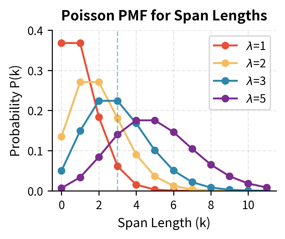
Sample span lengths: Draw span lengths from a Poisson distribution with parameter (typically ). This creates spans of varying sizes: many single-token spans, some two-token spans, fewer three-token spans, and so on. The Poisson distribution provides a natural way to generate this variety with a single parameter controlling the expected length.
-
Sample span positions: Randomly select starting positions for spans until approximately of the total tokens are covered by spans. The sampling continues until the target corruption level is reached, ensuring consistent corruption intensity across documents of different lengths.
Each span, regardless of length, is replaced with exactly one [MASK] token:
where:
- : a contiguous span of tokens starting at position
- : a single mask token that replaces the entire span
- : indicates the replacement operation
This many-to-one mapping is the crucial innovation. A single [MASK] in the input might correspond to zero tokens, one token, three tokens, or even more in the output. The model cannot simply count masks and produce the same number of tokens. It must learn to judge, from context alone, how extensive each gap is.
For example, "The quick brown fox jumps over the lazy dog" might become "The [MASK] fox [MASK] the [MASK] dog" where:
- "[MASK]₁" replaces "quick brown" (2 tokens)
- "[MASK]₂" replaces "jumps over" (2 tokens)
- "[MASK]₃" replaces "lazy" (1 token)
The decoder must figure out that the first mask needs two tokens (an adjective pair), the second needs two (a verb phrase), and the third needs one (a single adjective), all from the contextual clues in "The ... fox ... the ... dog."
The Poisson Distribution for Span Lengths
Why use Poisson? We want span lengths that vary naturally, mostly short spans with occasional longer ones, without needing to set a maximum length. The Poisson distribution is ideal because it models counts of independent events and has a single parameter controlling the average. This is convenient: rather than specifying an entire distribution over possible lengths, we tune one number and get a reasonable distribution automatically.
The Poisson distribution gives the probability of observing exactly events:
where:
- : the probability of observing exactly events (here, a span of tokens)
- : the span length (number of tokens, can be 0, 1, 2, ...)
- : the expected (average) span length, set to 3 in BART
- : the exponential decay factor ensuring probabilities sum to 1
- : factorial of , which appears because ordering doesn't matter within the span count
The formula works as follows: makes longer spans increasingly likely as grows.if the average is higher, we should see more long spans. Meanwhile, in the denominator penalizes very long spans (since factorial grows faster than exponential), preventing the distribution from placing too much mass on extremely long spans that would destroy too much context. The term normalizes everything to sum to 1, ensuring we have a valid probability distribution. Together, these three components create a distribution peaked near with a long tail toward higher values.
With :
- : 5% of spans have length 0 (insertions!)
- : 15% single-token spans
- : 22% two-token spans
- : 22% three-token spans
- : 36% longer spans
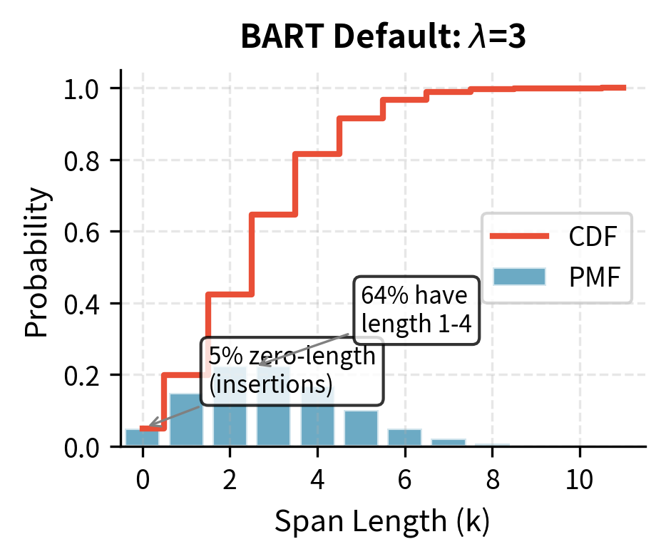
The inclusion of zero-length spans is particularly clever and deserves special attention. A zero-length span means inserting a [MASK] token between two existing tokens without removing anything. The decoder must learn to generate empty content for this mask.to recognize that sometimes a mask is a false alarm requiring no output. This teaches the model that not every mask needs to expand into content, a nuance absent from standard masking approaches where every mask always corresponds to exactly one token.
What the Model Learns
Text infilling develops generation capabilities that transfer directly to downstream tasks:
-
Length prediction: The model must infer how many tokens each mask represents. A single mask might expand to zero, one, five, or more tokens. This requires understanding semantic and syntactic constraints.
-
Coherent multi-token generation: Generating "quick brown" as a unit requires understanding that these words form a coherent phrase modifying "fox." The model cannot generate each token independently.
-
Span boundary detection: The model must determine where masked content ends and original content resumes. When generating tokens for a mask, the model must decide when to stop generating.
This directly addresses a limitation of T5's span corruption. T5 uses sentinel tokens that indicate span boundaries and generates only the corrupted spans with their sentinels. BART must reconstruct the full original text, interleaving generated and copied content smoothly. This trains the model for generation tasks where the output blends novel phrases with material from the input. This is exactly what happens in summarization, paraphrasing, and many other applications.
The corrupted sequence is notably shorter than the original. Each [MASK] might represent multiple tokens, so the decoder must learn to expand these placeholders appropriately. This many-to-one corruption followed by one-to-many generation is central to BART's effectiveness on generative tasks.
Sentence Permutation
Moving from token-level to structural corruption, sentence permutation shuffles the order of sentences within a document. This tests the model's understanding of discourse coherence and document structure.aspects of language that token-level corruptions cannot address. Well-written documents have logical flow: ideas build on each other, references point backward to established concepts, and conclusions follow from premises. Sentence permutation disrupts this flow and asks the model to restore it.
How It Works
The document is first segmented into sentences (typically using punctuation heuristics or a sentence tokenizer, as covered in Part I). These sentences are then randomly permuted:
where:
- : the corrupted document with reordered sentences
- : the original document as a sequence of sentences
- : a random permutation function that reorders the sentences
The shuffle operation creates a random permutation of the sentences, selecting uniformly from all possible orderings. For a three-sentence document, there are possible orderings, and each has equal probability of being selected. For example, a three-sentence document might be reordered from to , placing what was the middle sentence first and the original first sentence last.
What the Model Learns
Sentence permutation teaches document-level coherence in several ways:
-
Discourse relations: How does one sentence logically follow another? Causal relationships ("Because X, therefore Y"), temporal sequences ("First X, then Y"), and elaboration patterns ("X. More specifically, Y") all provide cues for ordering. The model must recognize these implicit connections even when discourse markers are absent.
-
Referential coherence: Pronouns and definite references ("the man," "this idea") typically follow their antecedents. Permuted text disrupts these chains.a sentence might use "he" before the person has been introduced, or mention "this approach" before the approach has been described. The model learns to recognize and restore proper reference chains.
-
Topic flow: Well-organized text develops ideas progressively. Opening sentences introduce topics; middle sentences elaborate; closing sentences conclude or transition. The model learns to recognize these structural roles and restore this flow.
However, sentence permutation alone proved less effective than token-level corruption in BART's experiments. The learning signal is sparse (each training example provides only a few reordering decisions), and many permutations might be equally valid for loosely connected sentences. A document with three independent observations could be reasonably ordered in any sequence, providing ambiguous signal to the model.
The permuted version reads awkwardly.the chronological and logical flow is disrupted. The decoder must restore proper ordering based on discourse cues.
Document Rotation
Document rotation is the most aggressive structural corruption in BART's repertoire. A random token is selected as the new starting point, and the document is rotated so that it begins with that token. Unlike sentence permutation, which at least preserves sentence boundaries, document rotation can split sentences arbitrarily, placing sentence fragments at the beginning or end.
How It Works
Given a document with tokens , we uniformly sample a position and rotate:
where:
- : the rotated (corrupted) document
- : the original document with tokens
- : the randomly chosen rotation point (sampled uniformly from 1 to )
- : tokens from position to the end become the new beginning
- : tokens before position are moved to the end
Think of the document as arranged in a circle. We pick a random position and "cut" the circle there, then lay it out linearly starting from that cut point. All tokens remain in their relative order, but the absolute positions shift. The original beginning might now appear in the middle or at the end.
For example, "The quick brown fox jumps" with becomes "brown fox jumps The quick." The fragment "brown fox jumps" appears first, followed by "The quick".a clear violation of sentence structure that signals something is wrong.
What the Model Learns
Document rotation teaches the model to identify document boundaries, specifically where a coherent document actually begins. This seems like a narrow skill, but it has practical uses:
-
Document structure recognition: Real documents have clear beginnings (titles, topic sentences) and endings (conclusions, sign-offs). The model learns to recognize these structural markers (capitalized first words, sentence-initial positions, opening phrases like "In this paper" or "The purpose of") that distinguish genuine document starts from arbitrary mid-document positions.
-
Global coherence: Unlike sentence permutation, which preserves some local structure, rotation can place mid-sentence fragments at document boundaries. The model must recognize incomplete thoughts, such as a sentence missing its subject or a phrase without context, as evidence of artificial boundaries.
In practice, document rotation was the least effective corruption scheme when used alone. The task is difficult (many rotation points produce plausible-looking starts, especially in long documents where sentence-initial positions are common), and the learning signal is limited to identifying a single boundary per document. The model receives one bit of useful information per training example: where the true start is.
The rotated sequence maintains word order within the two fragments but loses the natural starting point. The decoder must identify "The" as the true document beginning.
Combining Corruption Schemes
BART's key experimental contribution was systematically testing different combinations of these corruption schemes. Not all combinations are equally effective, and some corruptions complement each other while others are redundant. Understanding these interactions helps explain BART's final design choices and provides guidance for future model development.
Experimental Findings
The BART paper evaluated combinations across several downstream tasks. Key findings include:
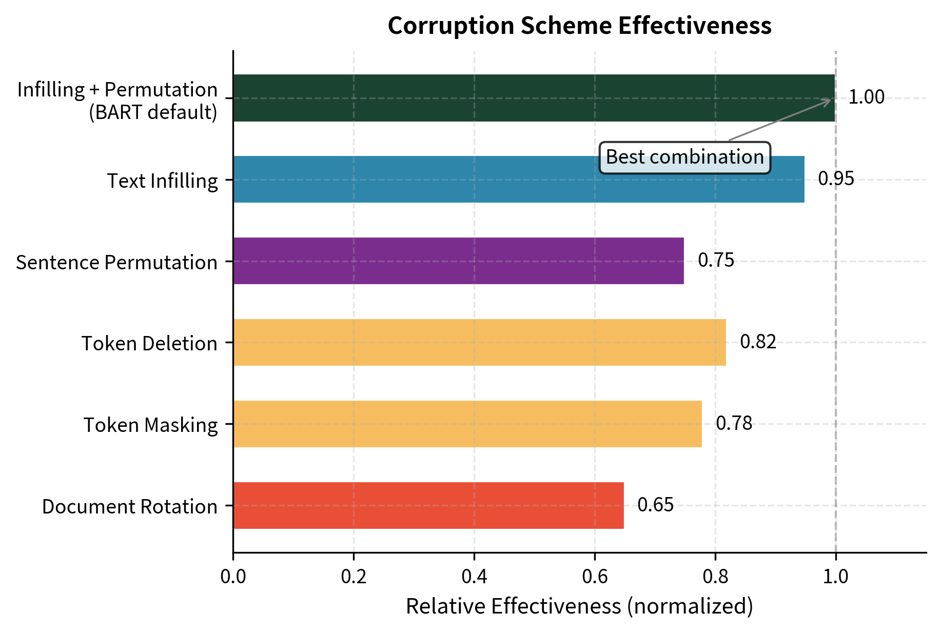
Text infilling dominates. When used alone, text infilling matched or exceeded other single-scheme corruptions across most tasks. The combination of length prediction and span reconstruction provides strong learning signals that transfer effectively to generation tasks.
Sentence permutation adds modest gains. Combining text infilling with sentence permutation slightly improved results on some tasks, particularly those requiring document understanding. However, the gains were small compared to infilling alone.
Token deletion is redundant with infilling. Text infilling subsumes token deletion because zero-length spans in infilling are equivalent to deletions. Combining them provides little benefit.
Document rotation hurts performance. Adding document rotation to other schemes generally degraded results. The task may be too difficult or too different from downstream applications.
Token masking alone is inferior. Pure masking performs worse than infilling because it cannot teach length prediction. Each mask always corresponds to exactly one token.
The Final BART Recipe
Based on these experiments, the standard BART pre-training uses:
- Text infilling with and approximately 30% of tokens in corrupted spans
- Sentence permutation applied to all documents
This combination balances local token prediction with global structure learning while avoiding the problems with rotation and the redundancy of separate deletion.
The combined corruption produces text that is both structurally shuffled and locally corrupted. The decoder faces the full challenge of restoring both sentence order and masked content.
Comparison with Other Pre-training Approaches
Understanding BART's pre-training requires comparing it to related approaches we've covered in earlier chapters.
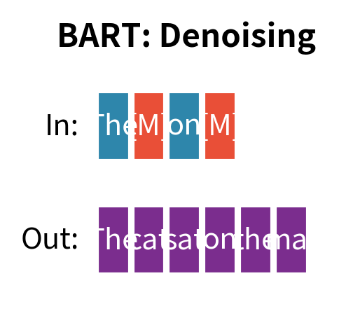
BART vs. BERT
BERT's masked language modeling (covered in Part XVII) masks 15% of tokens and predicts only those positions. Key differences:
| Aspect | BERT | BART |
|---|---|---|
| Architecture | Encoder-only | Encoder-decoder |
| Output | Masked positions only | Full sequence |
| Mask-to-token ratio | 1:1 | Variable (many:many) |
| Position signals | Mask tokens mark positions | No explicit position markers |
| Generation capability | Limited | Native |
BERT performs well at tasks requiring bidirectional understanding, such as classification and extraction, but struggles with generation because it was never trained to produce full sequences. BART maintains BERT's bidirectional encoder benefits while adding generation capability.
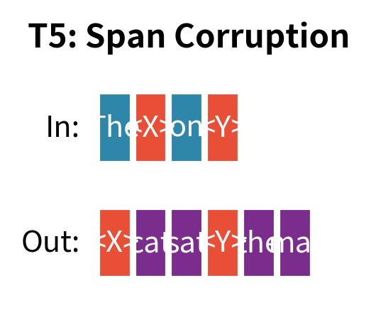
BART vs. T5
T5's span corruption (covered in Part XX, Chapter 2) shares BART's span-based approach but differs in key ways:
| Aspect | T5 | BART |
|---|---|---|
| Corruption output | Replace spans with sentinels | Replace spans with single mask |
| Decoder output | Only corrupted spans | Full original sequence |
| Span identification | Sentinels mark boundaries | No explicit boundaries |
| Training signal | Only corrupted tokens | All tokens |
T5's sentinel-based approach is more efficient, but BART's full-sequence reconstruction provides better signal for tasks requiring exact output control, such as grammatical error correction or style transfer.
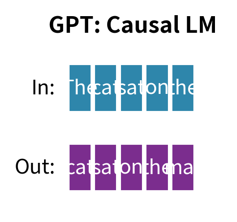
BART vs. GPT
GPT's causal language modeling (Part XVIII) trains the model to predict the next token given all previous tokens. Comparing to BART:
| Aspect | GPT | BART |
|---|---|---|
| Input corruption | None (left context only) | Various noising schemes |
| Attention | Causal (unidirectional) | Encoder bidirectional, decoder causal |
| Learning signal | Next token prediction | Full reconstruction |
| Zero-shot capability | Strong | Moderate |
GPT's unidirectional approach prevents it from using future context during encoding. BART's encoder sees the full corrupted input bidirectionally, which helps for tasks where understanding the complete input matters.
Implementation: Full Pre-training Data Pipeline
Let's implement a complete data pipeline for BART pre-training, showing how to process documents into training batches.
The BARTCorruptor class encapsulates the full corruption pipeline. The source text shows the combined effect of sentence permutation and text infilling: sentences appear in a different order with mask tokens replacing spans of varying lengths. The target remains the original text that the decoder must learn to reconstruct. In a real implementation, you would integrate this with a tokenizer (as covered in Part V) and batch multiple examples together.
Key Parameters
The key parameters for BART pre-training corruption are:
- mask_ratio: Fraction of tokens to corrupt (default 0.30). Higher values create more challenging reconstruction tasks but may remove too much signal.
- poisson_lambda: Mean of the Poisson distribution for span lengths (default 3.0). Controls average span size; higher values create longer spans.
- mask_token: Special token replacing corrupted spans. Must match the tokenizer's mask token.
- apply_sentence_permutation: Whether to shuffle sentence order before infilling. Enables document-level structure learning.
Visualizing Corruption Density
Understanding how different corruption schemes distribute their modifications helps build intuition about what the model learns.
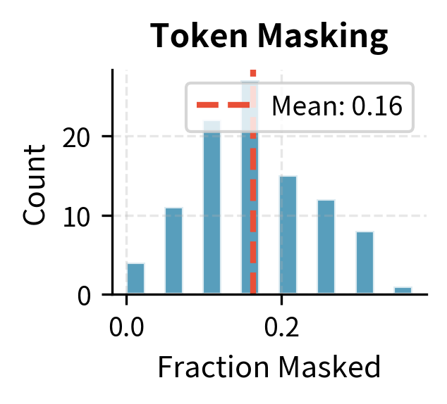
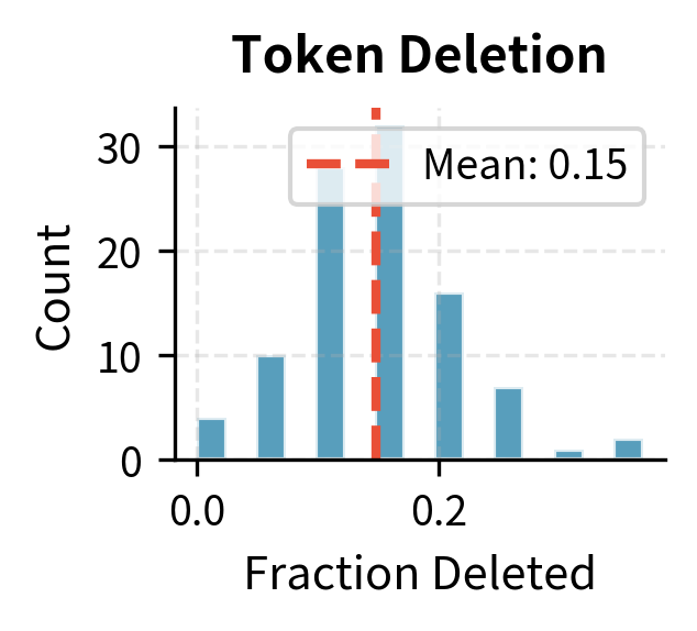
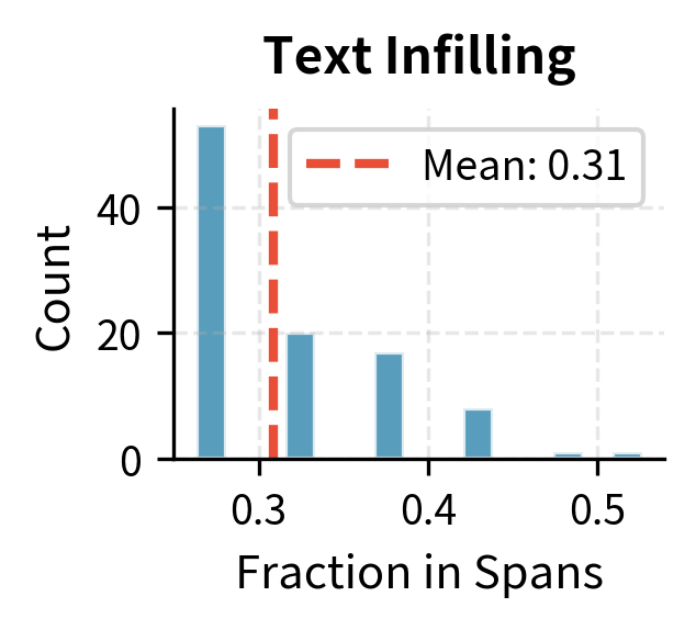
Token masking and deletion show similar distributions centered around their target probability. Text infilling affects more tokens (30% target) and shows higher variance due to the stochastic span lengths.some samples have many short spans while others have fewer long spans.
Training Dynamics
BART's pre-training uses standard practices for large language models, with some choices informed by its architecture:
Optimizer: AdamW with , , weight decay of 0.01. AdamW properly decouples weight decay from the adaptive learning rate.
Learning rate schedule: Linear warmup for the first 10,000 steps, then linear decay. This follows the pattern we saw in BERT pre-training but with a longer warmup suitable for larger models.
Batch size: Large batches (8,000 tokens per batch for BART-Base) improve training stability and allow higher learning rates.
Data: BART was trained on the same data as RoBERTa: 160GB of text including books, Wikipedia, news, and web text. This diverse corpus exposes the model to varied writing styles and domains.
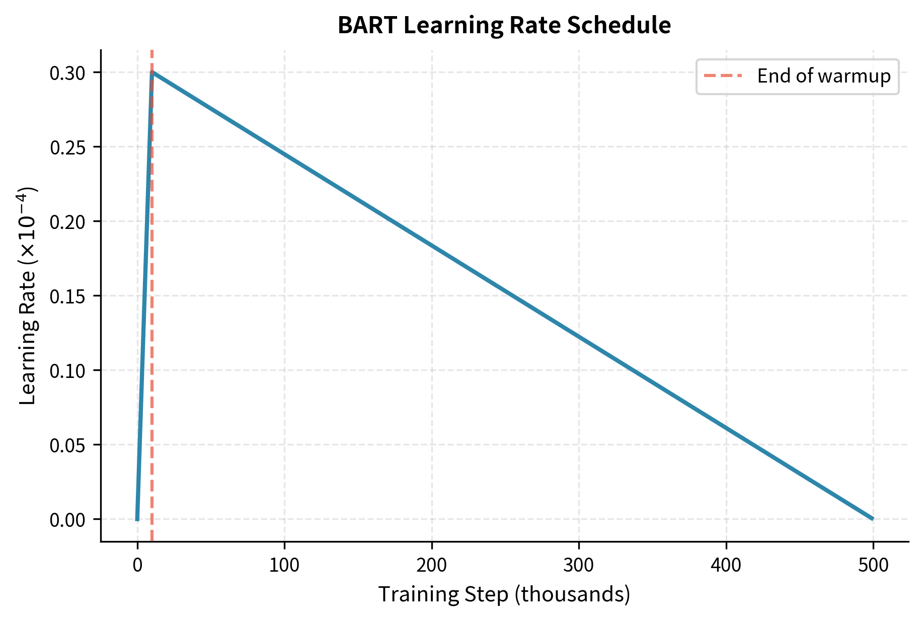
The warmup phase prevents early training instability when gradients are noisy and model weights are randomly initialized. The subsequent decay helps the model converge to a stable minimum.
Limitations and Impact
BART's pre-training approach has limitations that shaped subsequent research.
The full-sequence reconstruction objective is computationally expensive. Unlike T5, which generates only corrupted spans, BART's decoder processes every token of the original sequence. For long documents, this increases training cost significantly. The autoregressive decoder also prevents parallelization during training, unlike the encoder which processes all positions simultaneously.
The fixed corruption scheme may not be optimal for all downstream tasks. BART's text infilling with sentence permutation works well for summarization and generation, but other corruptions might better suit specific applications. More recent work has explored task-adaptive pre-training.
BART's bidirectional encoder limits its effectiveness for pure language modeling tasks. The model cannot directly perform next-token prediction like GPT because its encoder expects to see corrupted versions of complete sequences, not prefixes of text. This makes BART less suitable for applications requiring left-to-right generation from prompts without conditioning input.
Despite these limitations, BART demonstrated that encoder-decoder models could match or exceed BERT and GPT on their respective strengths by using appropriate pre-training corruptions. This finding influenced subsequent work on unified models that handle diverse tasks within a single architecture.
The span-based corruption approach has proven durable. Modern models continue to use variants of span corruption, with innovations focusing on how to select span boundaries, what to replace spans with, and how to balance local and global corruptions. The core idea remains central to pre-training design.
Summary
BART's pre-training strategy frames language model training as denoising autoencoding. By systematically exploring five corruption schemes, the researchers identified effective combinations for learning both local token patterns and global document structure.
Text infilling proved to be the most important individual corruption, teaching the model to predict how many tokens each mask represents and to generate coherent multi-token spans. Sentence permutation adds modest gains for tasks requiring document-level understanding. The final BART recipe combines these two approaches while avoiding less effective corruptions.
The key design choices that distinguish BART from related approaches are:
- Full-sequence reconstruction: Unlike T5, BART generates the complete original text, providing training signal for every position
- Variable-length spans: Unlike BERT's one-to-one masking, BART's infilling teaches length prediction through many-to-one corruption.
- Combined structural and local corruption: Sentence permutation addresses discourse while infilling addresses token-level prediction
These pre-training choices directly enable BART's strong performance on generation tasks such as summarization, translation, and dialogue.

Comments