

Learn BART's encoder-decoder architecture combining BERT and GPT designs. Explore attention patterns, model configurations, and implementation details.

This article is part of the free-to-read Language AI Handbook
Choose your expertise level to adjust how many terms are explained. Beginners see more tooltips, experts see fewer to maintain reading flow. Hover over underlined terms for instant definitions.
BART Architecture
BART (Bidirectional and Auto-Regressive Transformers) combines ideas from two main approaches in language modeling. When Facebook AI Research (now Meta AI) introduced BART in 2019, the NLP landscape was divided between encoder-only models like BERT, which excelled at understanding tasks, and decoder-only models like GPT, which dominated generation. BART asked a simple question: what if we combined the best of both worlds?
The answer turned out to be remarkably effective. BART uses a standard encoder-decoder architecture, based on a key insight: You can pre-train this architecture by corrupting text in arbitrary ways and then learning to reconstruct the original. This denoising approach proved especially powerful for tasks that require both understanding input and generating coherent output, such as summarization, translation, and question answering.
Where T5, which we covered in previous chapters, takes an encoder-decoder approach with a specific span corruption objective, BART uses a more flexible approach. It uses the same architectural building blocks but makes different choices about normalization, activation functions, and how pre-training objectives are structured. These differences matter in practice, leading to distinct strengths for different applications.
The BART Encoder-Decoder Design
BART follows the encoder-decoder framework we discussed in Part IX and Part XIII, but its design philosophy draws explicitly from BERT and GPT. To appreciate this design choice, consider the basic trade-off in language modeling: understanding requires seeing the full context (including what comes before and after a word), while generation must proceed sequentially since you cannot use words you have not yet produced. These two requirements seem contradictory, yet both are essential for tasks like summarization where you must deeply understand a document before producing a coherent condensed version.
BART resolves this tension through architectural separation. The encoder is essentially a BERT-style transformer, using bidirectional self-attention over the input sequence and allowing each token to attend to all other tokens. This bidirectional view means that when the encoder processes the word "bank" in a sentence, it can simultaneously consider both the preceding context ("walked along the") and the following context ("of the river") to determine that we're discussing a riverbank rather than a financial institution. The decoder, in contrast, is essentially a GPT-style transformer, using causal (left-to-right) self-attention to ensure the model can only use previously generated tokens when predicting the next one. This constraint is not a limitation, but a necessity. During generation, future tokens simply don't exist yet.
The architecture can be summarized as:
where:
- : the attention mask matrix of shape
- : the length of the input sequence
- Each entry of 1 indicates that attention is permitted between that query-key pair
This shows that BART's architecture combines two components: an encoder following BERT's bidirectional design, and a decoder following GPT's autoregressive design. The "+" here represents architectural composition rather than mathematical addition. The encoder and decoder are connected through cross-attention, a mechanism that allows the decoder to query the encoder's representations as it generates each token.
This formulation isn't just a metaphor. The BART authors explicitly designed the encoder to match BERT's architecture and the decoder to match GPT's, then connected them with cross-attention. This means BART inherits the bidirectional contextual understanding that made BERT successful for classification and extraction tasks, while also gaining the autoregressive generation capabilities that made GPT successful for text generation. The result is a model that can first build a rich, context-aware representation of the input, then leverage that representation to generate fluent, coherent output.
Encoder Structure
The BART encoder processes the input sequence using standard transformer encoder blocks, transforming raw token embeddings into contextualized representations. These representations capture the meaning of each token within its full surrounding context. Each block contains:
-
Multi-head self-attention with bidirectional (non-causal) masking. This is the mechanism that allows each token to "see" every other token in the input, gathering information from both directions to build context-aware representations.
-
Feed-forward network with GeLU activation. After attention aggregates information across positions, this two-layer neural network transforms each position's representation independently, allowing the model to compute complex non-linear functions of the attended information.
-
Residual connections around both sublayers. These skip connections add the input of each sublayer to its output, creating direct gradient pathways that facilitate training deep networks and allowing the model to learn incremental refinements rather than complete transformations.
-
Layer normalization applied after each sublayer (post-norm). This normalizes the activations to have zero mean and unit variance, stabilizing training by preventing the hidden representations from growing too large or too small as they pass through many layers.
The encoder produces a sequence of hidden states, one for each input token. These states capture rich bidirectional context, as each encoder representation can incorporate information from the entire input sequence. When you pass a sentence through BART's encoder, the representation for each word includes its meaning within the sentence context.
Decoder Structure
The decoder generates output tokens autoregressively, one at a time, using the encoder's representations to understand the input. This process mirrors how a human might write a summary. First, you read and understand the source document, which corresponds to the encoder. Then you compose the summary word by word while referring back to the original. This corresponds to the decoder with cross-attention. Each decoder block contains:
-
Causal self-attention over previously generated tokens. This allows each position to attend only to earlier positions in the output sequence, building up a representation of what has been generated so far. The causal constraint ensures the model cannot "cheat" by looking at tokens it hasn't yet produced.
-
Cross-attention over encoder hidden states. This is the bridge between understanding and generation. It allows the decoder to query the encoder's representations, focusing on different parts of the input as needed for generating each output token.
-
Feed-forward network with GeLU activation. Just as in the encoder, this transforms the combined self-attention and cross-attention information through a non-linear function.
-
Residual connections around all three sublayers. With three sublayers instead of two, the decoder has even more opportunity to benefit from these direct pathways that preserve information and facilitate gradient flow.
-
Layer normalization after each sublayer (post-norm). This maintains training stability across the decoder's deeper structure.
The causal masking in self-attention prevents the decoder from "cheating" by looking at future tokens during training. When training on a target sequence like "The study found significant results," the decoder predicting "found" can see "The" and "study" but not "significant" or "results." Cross-attention allows each decoder position to attend to all encoder positions, enabling the decoder to ground its generation in the input context. When generating "found," it can look back at the relevant parts of the source document.
Key Architectural Choices
BART makes several design decisions that distinguish it from other encoder-decoder models. These choices reflect its heritage from BERT and GPT and affect training dynamics and model behavior.
-
GeLU activation: Unlike T5, which uses ReLU, BART follows BERT and GPT-2 in using the GeLU (Gaussian Error Linear Unit) activation function in feed-forward layers. GeLU provides smoother gradients than ReLU because it doesn't have a sharp transition at zero. Instead, it smoothly interpolates between passing and blocking signals. This smoothness can lead to more stable optimization and has become the preferred activation for many modern language models.
-
Post-layer normalization: BART applies layer normalization after residual connections (known as post-norm), following the original transformer design. T5 uses pre-norm, applying layer normalization before each sublayer. The placement of normalization affects gradient flow. Pre-norm tends to produce more stable gradients at initialization, making it easier to train very deep models. Post-norm can achieve slightly better final performance when training succeeds. This trade-off explains why both conventions persist in practice.
-
Learned positional embeddings: BART uses learned absolute position embeddings, similar to BERT and GPT-2, rather than the relative position encodings used in T5. With learned embeddings, the model maintains a separate embedding vector for each position (1, 2, 3, and so on up to some maximum), and these vectors are learned during training. This approach is simple and effective but creates a hard limit on sequence length. The model has no embedding for position 1025 if it was trained with a maximum of 1024.
-
No parameter sharing: Unlike T5, BART does not tie encoder and decoder embeddings by default. The encoder and decoder maintain separate embedding matrices. This increases parameter count but allows the encoder and decoder to learn specialized representations suited to their different roles (understanding versus generation).
Attention Configuration
BART's attention patterns show how information flows through the model. Attention is the mechanism by which transformers route information between positions, and the pattern of allowed attention, which positions can attend to which other positions, fundamentally shapes what the model can learn and compute. Let's examine each attention mechanism in detail, building intuition for why each pattern exists and how it serves the model's goals.
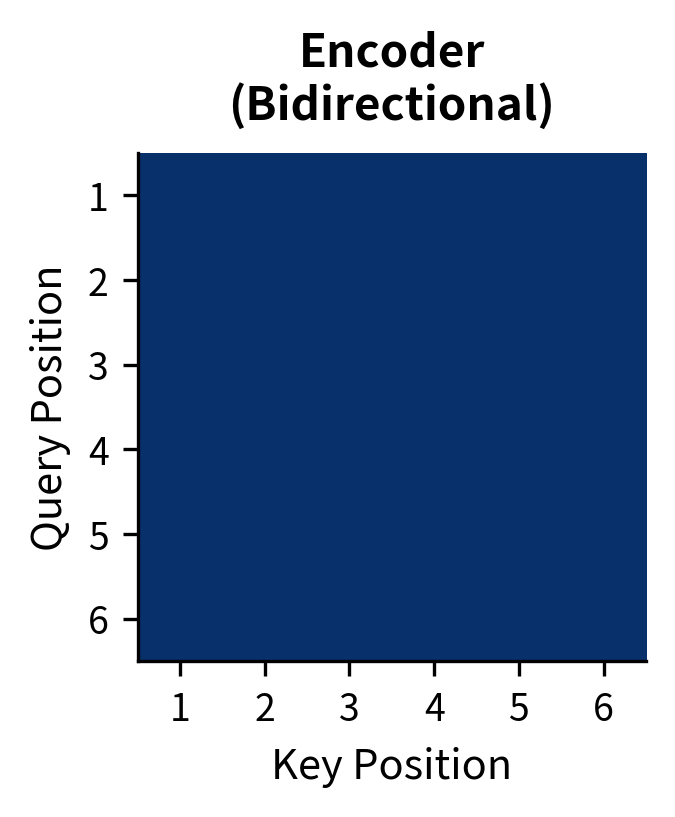
Encoder Self-Attention
In the encoder, every token can attend to every other token. This bidirectional attention gives the encoder the power to build contextual representations, because a word's meaning often depends on context that appears both before and after it. Consider disambiguating "The bank was eroding" versus "The bank was closing"; you need both the subject and the verb to understand which sense of "bank" is intended.
For an input sequence of length , the attention mask is an matrix of ones:
where:
- : the attention mask matrix of shape
- : the length of the input sequence
- Each entry of 1 indicates that attention is permitted between that query-key pair
Reading this matrix, row describes which positions token can attend to: a 1 in column means token can attend to token . Since every entry is 1, every token can attend to every other token, including itself. This complete connectivity allows information to flow freely through the sequence, enabling the encoder to build representations that incorporate arbitrarily distant context.
This bidirectional attention is what gives encoder-only models like BERT their power for understanding tasks. Each token's representation is informed by the complete context, not just preceding tokens. A word at the beginning of a sentence can be influenced by words at the end, and vice versa, enabling the rich contextual representations that make BERT effective for tasks like sentiment analysis and named entity recognition.
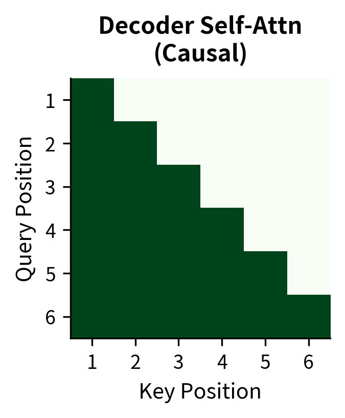
Decoder Causal Self-Attention
The decoder uses causal (or autoregressive) masking in its self-attention layers. The word "causal" refers to the structure of language generation. Each token is caused by (depends on) the tokens that came before it, not those that come after. This constraint isn't artificial. During generation, future tokens don't yet exist.
For a sequence of length , the attention mask is a lower-triangular matrix:
where:
- : the causal attention mask matrix of shape
- : the length of the decoder sequence (tokens generated so far)
- Entry if , meaning position can attend to position , and 0 otherwise
The lower-triangular structure emerges directly from the causality constraint. Position 1 can only attend to position 1 (itself), so the first row has a single 1. Position 2 can attend to positions 1 and 2, giving two 1s. Position can attend to all positions from 1 through , creating the triangular pattern. The zeros above the diagonal represent the blocked attention to future positions, which is information that the model must not use because it won't be available at generation time.
This ensures that when generating token , the model can only attend to tokens at positions . This causal structure makes autoregressive generation possible. During training, we can compute attention for all positions in parallel (the mask handles the constraints), but the model learns to predict each token using only its predecessors, exactly as it will during generation.
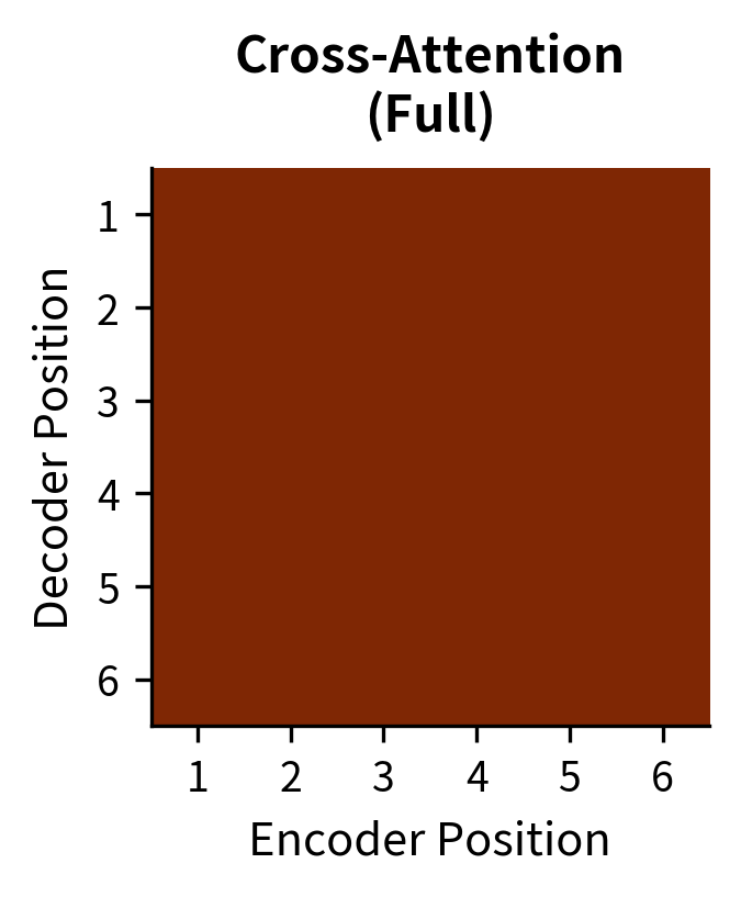
Cross-Attention
Cross-attention connects the decoder to the encoder, bridging the understanding and generation phases. Without cross-attention, the decoder would not know what input to generate output for. It would become an unconditional language model, generating plausible text without grounding in any specific input.
For each decoder position, queries come from the decoder hidden states while keys and values come from the encoder hidden states. This asymmetry is meaningful. The decoder is asking questions (represented as queries) about the input, and the encoder provides the answers (as values) along with ways to determine relevance (through keys). There is no masking in cross-attention; every decoder position can attend to every encoder position:
where:
- : query vectors derived from decoder hidden states, shape . These represent "what the decoder is looking for" at each position.
- : key vectors derived from encoder hidden states, shape . These represent "what information each encoder position offers" and are compared against queries.
- : value vectors derived from encoder hidden states, shape . These contain the actual information that will be retrieved and combined.
- : the dimension of query and key vectors (used for scaling)
- : the dimension of value vectors
- : scaling factor that prevents dot products from growing too large, which would push softmax into regions with vanishing gradients
The computation proceeds in three stages. First, the dot product computes a compatibility score between each decoder position and each encoder position, resulting in an matrix of raw attention scores. Second, the softmax operation converts these scaled scores into attention weights that sum to 1 across encoder positions. This is a proper probability distribution over the input, indicating how much attention each output position pays to each input position. Third, these weights are used to compute a weighted combination of encoder values, where positions with higher attention weights contribute more to the final representation.
This lets the decoder "look at" different parts of the input when generating each output token. When summarizing a document, the decoder might focus on the introduction when generating the first sentence of the summary, then shift attention to specific details when describing particular findings, and attend to the conclusion when wrapping up. This dynamic alignment is what makes encoder-decoder models so effective for conditional generation tasks.
This lets the decoder focus on different parts of the input as it generates each output token, a mechanism we explored thoroughly in our discussion of Bahdanau and Luong attention in Part IX.
Attention Flow Visualization
To understand how information flows through BART, consider processing an input sequence and generating an output. The flow follows a clear two-phase structure that separates understanding from generation while connecting them through cross-attention.
-
Encoder phase: Input tokens are processed through encoder layers. At each layer, bidirectional self-attention allows information to flow freely between all positions. The input might be a long document. By the end of the encoder, each token's representation includes context from the entire document. This phase processes the entire input once, creating a fixed set of representations that the decoder will query.
-
Decoder phase: For each output token, the decoder performs a sequence of operations that integrate three sources of information:
- Causal self-attention integrates information from previously generated tokens, building a representation of the output generated so far
- Cross-attention retrieves relevant information from the encoder, grounding the generation in the input
- The feed-forward network transforms the combined representation, computing complex functions of the attended information
- The output projection produces a probability distribution over the vocabulary, from which the next token is selected
This two-phase structure is efficient for tasks with long inputs and shorter outputs. The expensive encoder computation happens once, and the decoder reuses those representations for every generated token.
BART vs T5 Comparison
BART and T5 were developed around the same time and share the encoder-decoder architecture, but they differ in key ways. Understanding these differences helps you choose the right model and shows the design options of encoder-decoder models more broadly.
Architectural Differences
The table below summarizes the key architectural distinctions:
| Component | BART | T5 |
|---|---|---|
| Activation function | GeLU | ReLU (original) / GeGLU (v1.1) |
| Normalization | Post-norm | Pre-norm |
| Position encoding | Learned absolute | Relative (bucketed) |
| Embedding sharing | Separate | Tied (encoder-decoder) |
| Vocabulary | BPE (GPT-2 tokenizer) | SentencePiece |
Pre-norm versus post-norm affects training stability. As we discussed in Part XII, pre-norm tends to produce more stable gradients at initialization, which can enable training larger models more easily. The key difference is where normalization occurs in the residual pathway. Pre-norm normalizes the input to each sublayer, ensuring that the residual connection adds a well-scaled update. Post-norm normalizes the output, which can lead to larger variations in the residual pathway. However, post-norm models often achieve slightly better final performance when training is successful, creating a trade-off between training ease and final quality.
BART's use of learned absolute position embeddings means it has a fixed maximum sequence length (typically 1024 tokens), while T5's relative position encoding theoretically generalizes to longer sequences. In practice, both models require additional techniques for handling very long contexts, as we covered in Part XV.
Input-Output Formatting
The most noticeable difference is how input and output are structured:
T5 uses a text-to-text format where every task is framed as mapping an input text to an output text. Tasks are specified through prefixes:
summarize: The researchers conducted experiments... → The study found...
translate English to German: Hello world → Hallo Welt
BART treats tasks more naturally. For sequence-to-sequence tasks like summarization, the input goes to the encoder and the output comes from the decoder. For classification tasks, a special token's representation from the decoder is used for prediction. This is closer to how BERT handles classification, where the [CLS] token representation is used.
Pre-training Objectives
While we'll cover BART's pre-training in detail in the next chapter, here are the high-level differences.
-
T5 uses span corruption, replacing random spans of tokens with sentinel tokens and training the model to generate the missing spans.
-
BART explores multiple noise functions: token masking, token deletion, text infilling, sentence permutation, and document rotation. The full document is reconstructed as output.
T5's span corruption is more computationally efficient because the target sequence is much shorter than the input. BART's document reconstruction means the target is the same length as the uncorrupted input, requiring more computation but providing a stronger training signal for generation tasks.
Performance Trade-offs
In benchmarks, both models show strong performance with different strengths:
- Summarization: BART tends to perform better, likely because its pre-training requires generating coherent, full-length text rather than filling in short spans.
- Translation: Performance is similar, with both models achieving strong results when fine-tuned on parallel data.
- Question answering: Both perform well, with specific results depending on the dataset and fine-tuning setup.
- Classification: BART can perform classification by using the decoder's representation of a special token, though encoder-only models remain competitive for pure classification.
The practical difference often comes down to implementation details and fine-tuning approach rather than architecture.
BART Model Sizes
BART was released in two primary sizes, following the naming convention established by BERT:
BART-base
The base model provides a good balance between capability and computational requirements.
- Encoder layers: 6
- Decoder layers: 6
- Hidden dimension: 768
- Attention heads: 12
- Feed-forward dimension: 3072
- Parameters: ~140 million
BART-base works well when computational resources are limited or fast inference is required. It can run on consumer GPUs and provides strong performance on tasks such as summarization and question answering.
BART-large
The large model increases capacity significantly.
- Encoder layers: 12
- Decoder layers: 12
- Hidden dimension: 1024
- Attention heads: 16
- Feed-forward dimension: 4096
- Parameters: ~400 million
BART-large performs better on most benchmarks, particularly for complex generation tasks. It requires more memory and computation, typically requiring a GPU with at least 16GB of memory for fine-tuning.
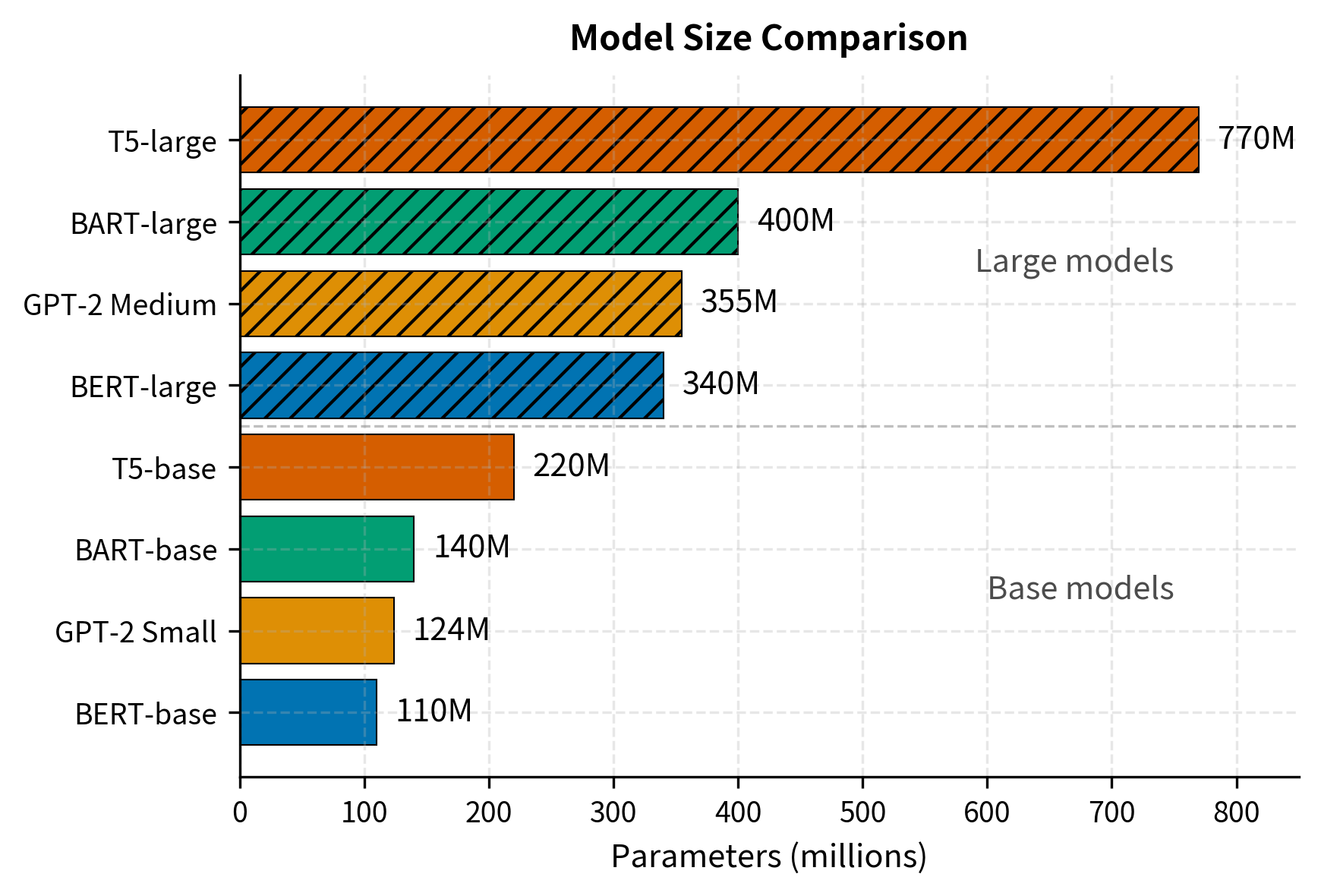
Comparison with Other Models
The following table contextualizes BART's sizes relative to related models:
BART's parameter count is somewhat lower than T5 for the same size label because T5 uses more layers. BART-large with 12+12 layers is closer to T5-base with 12+12 layers in terms of depth, though T5 uses parameter-efficient relative position encodings while BART has separate learned embeddings for each position.
Code Implementation
Let's explore BART's architecture using the Hugging Face Transformers library. We'll examine the model structure, inspect attention patterns, and see how the encoder and decoder interact.
First, let's examine the model configuration to confirm the architectural details we discussed:
The configuration confirms our discussion: 6 encoder and decoder layers, 768-dimensional hidden states, 12 attention heads, and GeLU activation. The maximum position embeddings of 1024 reflects BART's use of learned absolute position encoding, matching the architectural specifications from the BART paper.
Now let's pass an example through the model and examine the outputs:
The output shapes reveal the flow of information. The encoder produces hidden states for each input token, while the decoder produces hidden states for each position in the output sequence (currently just one, for the BOS token).
Let's visualize the attention patterns from the last layer of each component:
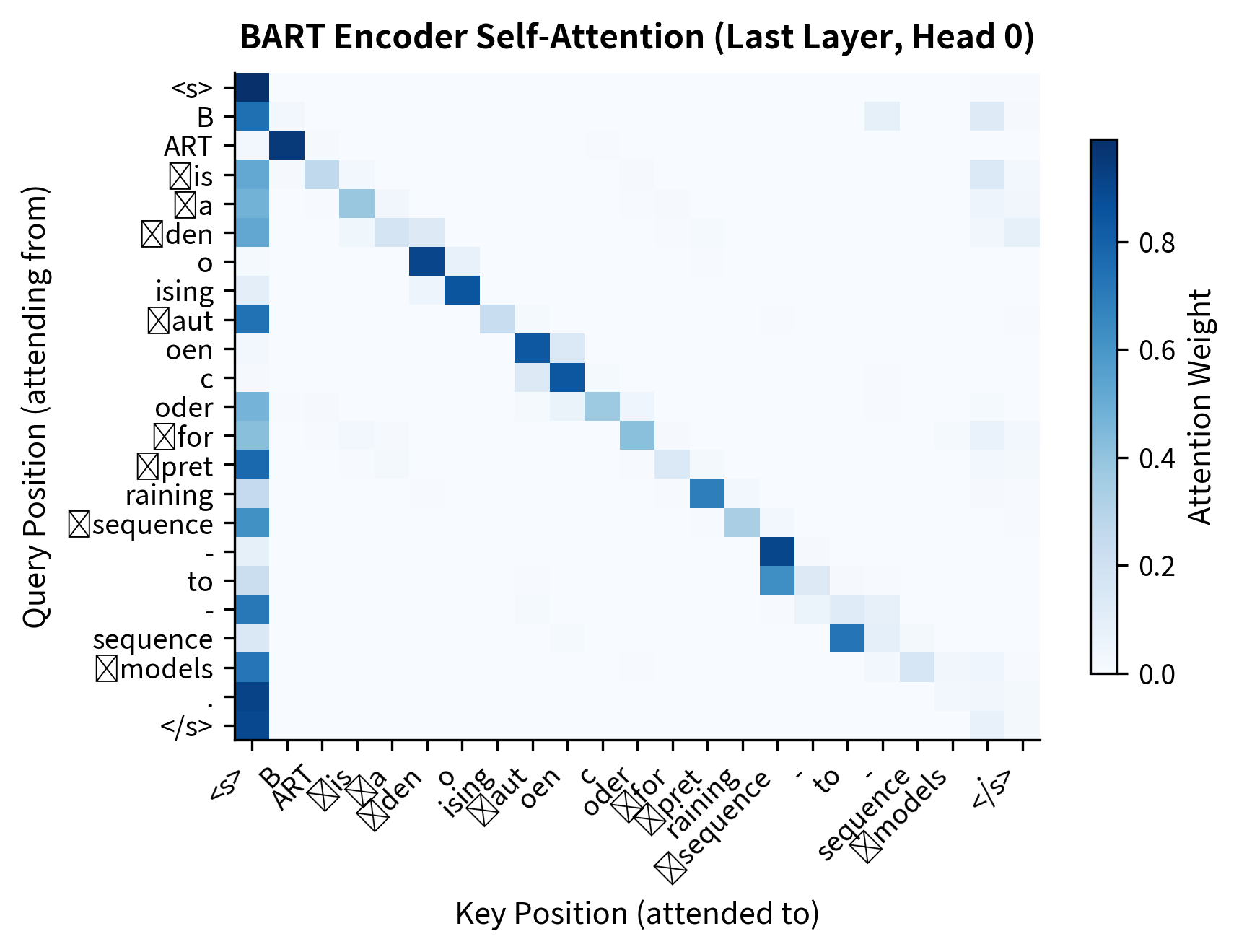
The encoder attention pattern shows the bidirectional nature of BART's encoder. Each token can attend to all other tokens, with the model learning to focus on contextually relevant positions.
Now let's examine cross-attention by generating a longer output sequence:
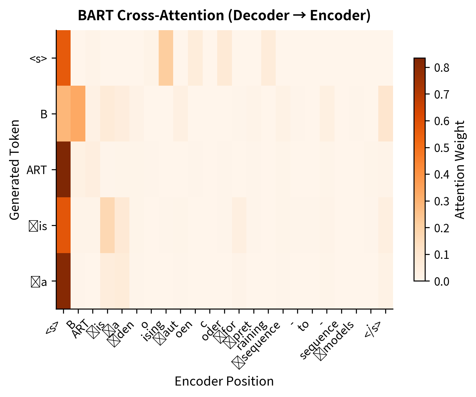
The cross-attention visualization reveals how the decoder grounds its generation in the input. Each row shows which encoder positions a generated token attended to, demonstrating the dynamic alignment between input and output.
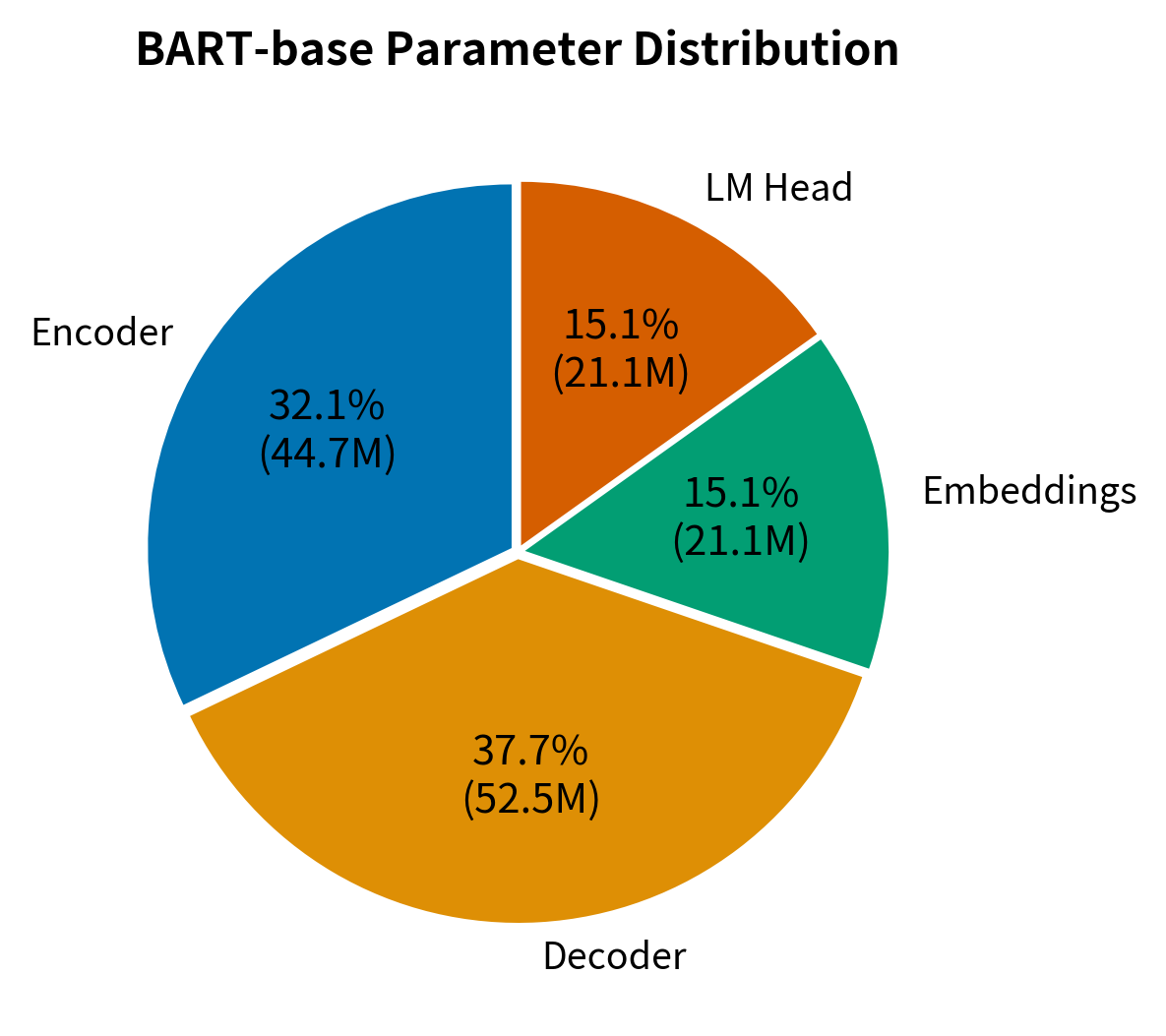
Let's also count parameters to verify the model sizes we discussed:
The parameter count confirms that BART-base has approximately 140 million parameters, split roughly evenly between the encoder and decoder with significant additional parameters in the embedding matrices. This aligns with our earlier discussion of BART model sizes and demonstrates how the encoder-decoder architecture distributes capacity across both components.
Key Parameters
The key parameters for BART's architecture are:
- d_model: The hidden dimension size, which is 768 for base and 1024 for large. Controls the representation capacity of the model.
- encoder_layers / decoder_layers: Number of transformer blocks in each component. More layers increase model capacity but also computational cost.
- encoder_attention_heads: Number of attention heads (12 for base, 16 for large). Multiple heads allow the model to attend to different aspects of the input simultaneously.
- encoder_ffn_dim: Dimension of the feed-forward network, typically 4 times the hidden dimension. Controls the capacity of the non-linear transformations.
- max_position_embeddings: Maximum sequence length the model can process (1024 for BART). Limited by learned absolute position embeddings.
- activation_function: The non-linearity used in feed-forward layers (GeLU for BART).
Limitations and Impact
BART's architecture has trade-offs to consider.
The post-norm design that BART inherited from the original transformer makes training less stable at large scales compared to pre-norm architectures. This is why T5 and most modern LLMs use pre-norm. When scaling BART beyond its original sizes, learning rate schedules and initialization require careful tuning.
The use of learned absolute position embeddings limits BART's ability to generalize to sequence lengths beyond those seen during training. While the model can process longer sequences by extending position embeddings, performance typically degrades. This contrasts with relative position encoding approaches such as those in T5 or the RoPE embeddings we covered in Part XI, which offer better length generalization.
Computationally, BART's pre-training objective requires reconstructing the entire input document, making pre-training more expensive than T5's span corruption approach. For downstream applications, however, this difference disappears since both models fine-tune and generate output tokens autoregressively.
Despite these limitations, BART had a major impact. It demonstrated that combining BERT-style encoding with GPT-style decoding produces a model that handles both understanding and generation well. The denoising pre-training framework opened new directions for exploring different corruption schemes, which we'll examine in the next chapter.
BART also showed that encoder-decoder architectures work well for conditional generation tasks. While decoder-only models like GPT have since dominated many applications due to their simplicity and scalability, encoder-decoder models like BART remain competitive for tasks where the input and output differ structurally, such as in document summarization or data-to-text generation.
Summary
BART combines a BERT-style bidirectional encoder with a GPT-style autoregressive decoder, creating a model for both understanding and generation. The encoder processes input with full bidirectional self-attention, while the decoder uses causal self-attention for generation and cross-attention to condition on the encoder's representations.
Compared to T5, BART makes different architectural choices. These include GeLU activation instead of ReLU, post-norm instead of pre-norm, learned absolute positions instead of relative positions, and separate embedding matrices for encoder and decoder. These differences reflect BART's design philosophy of directly combining proven components from BERT and GPT rather than exploring novel architectural variations.
BART comes in base (140M parameters) and large (400M parameters) configurations. Both use 12 attention heads in each layer and follow the same overall structure, differing only in depth and hidden dimensions.
The next chapter explores BART's pre-training in detail, examining the various noising functions that teach the model to reconstruct corrupted text and how these objectives shape the model's capabilities for downstream tasks.
Quiz
Ready to test your understanding? Take this quick quiz to reinforce what you've learned about BART's encoder-decoder architecture.

Comments