Liquidity Risk Management: Beyond VaR and Market Risk

Throughout Part V, we have focused on risks that can be measured through price movements: market risk captured by VaR and expected shortfall, credit risk modeled through default probabilities and loss given default, and counterparty risk quantified via CVA. These risks, while challenging to measure, share a common feature: they manifest through observable market prices or clearly defined credit events. However, some of the most devastating financial losses stem from risks that our pricing models do not capture well, risks that emerge precisely when our quantitative frameworks are most stressed.

Liquidity risk is perhaps the most insidious of these. It is not about prices moving against you, but about whether you can transact at all, and at what cost. A portfolio might show acceptable VaR under normal conditions, yet face catastrophic losses when the positions cannot be unwound without devastating price impact. The 2008 financial crisis demonstrated this vividly: assets that appeared liquid under normal conditions became nearly impossible to sell, turning paper losses into realized disasters.

Beyond liquidity, financial institutions face operational risks (losses arising from failed processes, systems, or human errors) and model risk, the danger that our quantitative tools themselves contain flaws or rest on invalid assumptions. These risks resist easy quantification, yet they have caused some of the largest losses in financial history. The collapse of Barings Bank from unauthorized trading, the London Whale's multi-billion dollar losses from mispriced derivatives, and the failure of sophisticated models during the subprime crisis all illustrate how non-market risks can overwhelm the careful calibrations of market risk models.

This chapter explores these risks that standard pricing models do not adequately address, examining how to measure what we can, manage what we cannot fully measure, and maintain healthy skepticism about our own quantitative frameworks.

Market liquidity refers to the ability to execute transactions quickly and at prices close to the asset's fundamental value. When liquidity is high, you can buy or sell large positions without significantly moving the market price. When liquidity is low, even modest trades can cause substantial price impact, eroding returns and potentially triggering cascading losses.

To understand why market liquidity matters so profoundly, consider the difference between owning an asset and being able to realize its value. A portfolio statement might show a position worth ten million dollars based on the last traded price, but this figure assumes you can actually sell at or near that price. In reality, the process of selling transforms the abstract concept of "value" into concrete cash, and that transformation is neither free nor instantaneous. Liquidity measures how smoothly and cheaply this transformation occurs.

The most immediately observable measure of liquidity is the bid-ask spread: the difference between the highest price buyers are willing to pay (bid) and the lowest price sellers are willing to accept (ask). This spread represents a direct transaction cost: to enter and immediately exit a position, you would lose the spread.

The intuition behind why the bid-ask spread exists is straightforward. Market makers and other liquidity providers face inventory risk when they accommodate traders. If you want to sell immediately, a market maker must buy from you and hold the inventory until another buyer arrives. During that holding period, the market maker bears the risk that prices will move against them. The spread compensates market makers for this risk, for the cost of maintaining their operations, and for the informational disadvantage they face when trading against potentially better-informed counterparties.

From a practical standpoint, the spread functions as an implicit tax on trading. Every time you enter a position, you pay half the spread (buying at the ask when the "true" price is the midpoint). When you exit, you pay the other half (selling at the bid). For active traders executing many transactions, these costs compound significantly. For long-term investors, the spread represents a one-time friction that diminishes in importance as the holding period lengthens.

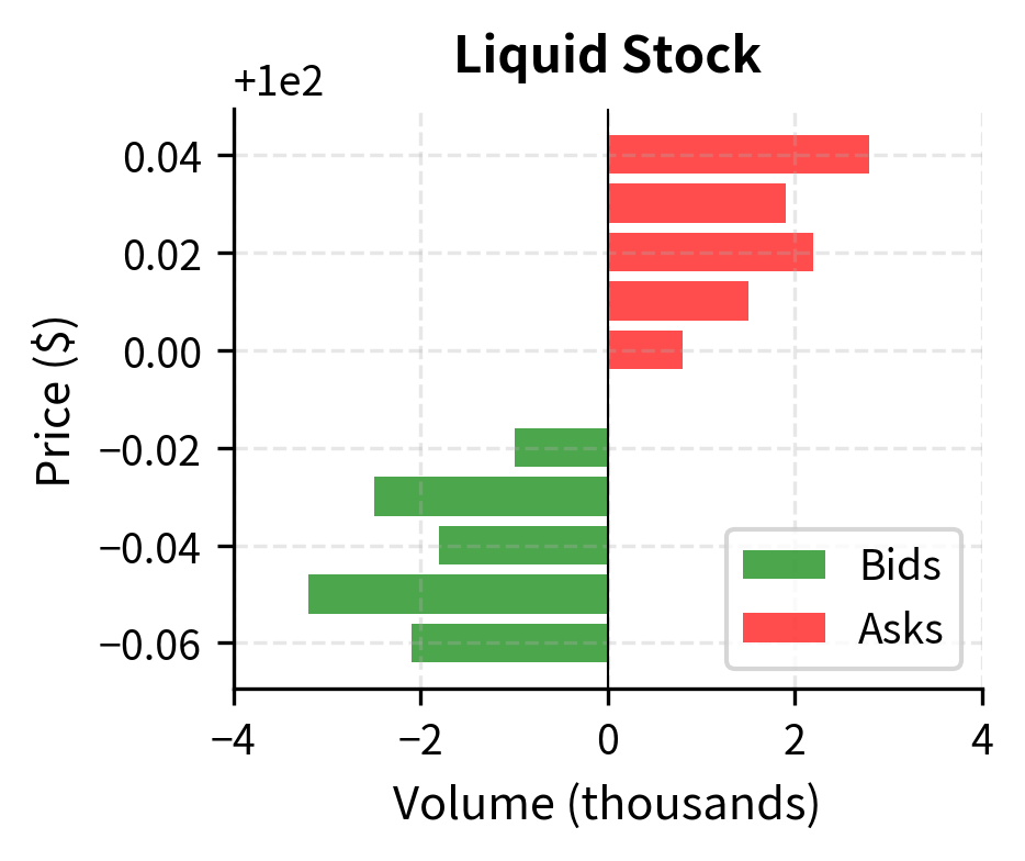
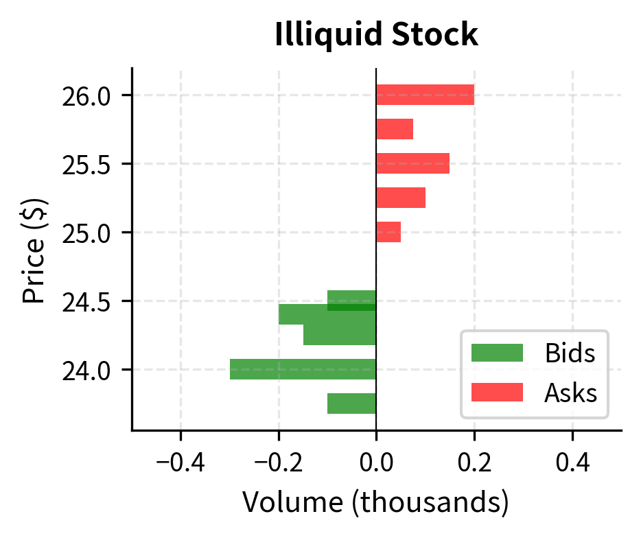
The liquid stock has a spread of just 2 cents (0.02%), while the illiquid stock shows a spread of 50 cents (2%). For a $1 million position, entering and exiting the liquid stock costs approximately $200 in spread costs, while the same round trip in the illiquid stock costs $20,000, a hundred-fold difference that can dramatically affect trading strategy profitability.

This hundred-fold difference in transaction costs has profound implications for portfolio management. A strategy that generates 50 basis points of alpha per trade might be highly profitable in liquid markets but utterly unprofitable in illiquid ones, where the spread alone consumes or exceeds the expected return. This is why quantitative trading strategies often focus exclusively on the most liquid instruments, and why institutional investors demand significant expected returns before venturing into less liquid asset classes.

The bid-ask spread captures only the cost of small trades. For larger orders, we must consider market depth: how much volume exists at each price level. Executing a large order "walks through the book," consuming liquidity at progressively worse prices.

The concept of market depth extends the intuition of the spread to larger transactions. Imagine a limit order book as a series of shelves, each holding a certain quantity of shares available at a particular price. The best bid shelf holds shares that buyers are willing to purchase at the highest price. The next shelf holds buyers at a slightly lower price, and so on. When you want to sell a large quantity, you must empty not just the first shelf but potentially many shelves, each at progressively less favorable prices.

This phenomenon creates what economists call "price impact": the tendency of trades to move prices against you. A large sell order exhausts buyers at high prices and must accept lower prices from buyers further down the book. The resulting average execution price will be worse than the initial quote, and the market price after the trade may remain depressed as the order reveals selling pressure to other market participants.

Understanding market depth requires thinking about both visible and hidden liquidity. The limit order book shows standing orders, but there may also be "iceberg" orders that reveal only a fraction of their true size, algorithmic traders who dynamically provide liquidity in response to market conditions, and potential buyers who would enter the market if prices became attractive. This hidden liquidity means that market depth is partially observable, adding uncertainty to execution cost estimates.

This analysis reveals a critical asymmetry. In the liquid stock, we can execute 10,000 shares with modest price impact. In the illiquid stock, we cannot even fill 1,000 shares from the available order book. We would exhaust visible liquidity and either wait for new orders to arrive or signal our demand through repeated attempts, likely pushing prices even higher.

The inability to execute at any price represents an extreme form of liquidity risk. In the illiquid stock example, if you have an urgent need to buy 1,000 shares, you face an impossible situation based solely on visible liquidity. You must either accept that your order cannot be filled immediately, thereby taking on timing risk, or you must signal your demand more aggressively, potentially attracting predatory trading behavior from others who recognize the urgency of your need.

Empirical research on market microstructure has established a remarkably consistent relationship between order size and price impact. The square-root law, observed across diverse markets and time periods, states that the permanent price impact of a trade scales with the square root of its size relative to typical trading volume.

The mathematical formulation of this relationship provides a practical tool for estimating execution costs before placing trades:

where:

• Impact: estimated price impact of the trade
• \sigma: asset's daily volatility
• Q: trade quantity
• V: average daily trading volume

This relationship implies that doubling your order size increases impact by only about 41%, not 100%, reflecting the market's ability to partially absorb larger orders over time.

To understand why the square-root relationship arises, consider the nature of price discovery in markets. Prices move because traders' demands reveal information about asset values. A large order suggests the trader has strong conviction, either because they possess private information or because they urgently need to transact. However, the information content does not scale linearly with order size. A trade of twice the size does not contain twice the information; rather, the incremental information in each additional share diminishes as the trade grows.

The presence of volatility in the formula reflects an important insight: price impact is fundamentally about how much your trade moves the market relative to how much the market moves on its own. In a highly volatile market where prices routinely swing several percent per day, a trade that moves prices by half a percent may be unremarkable. In a calm market, the same absolute price movement would be striking. The volatility term normalizes impact across different market regimes.

The participation rate, defined as your trade quantity divided by the average daily volume, captures how significant your trade is relative to the overall market activity. Trading 1% of daily volume is routine and unlikely to attract attention. Trading 50% of daily volume signals that something unusual is happening, drawing scrutiny from other participants and potentially triggering adverse selection effects.

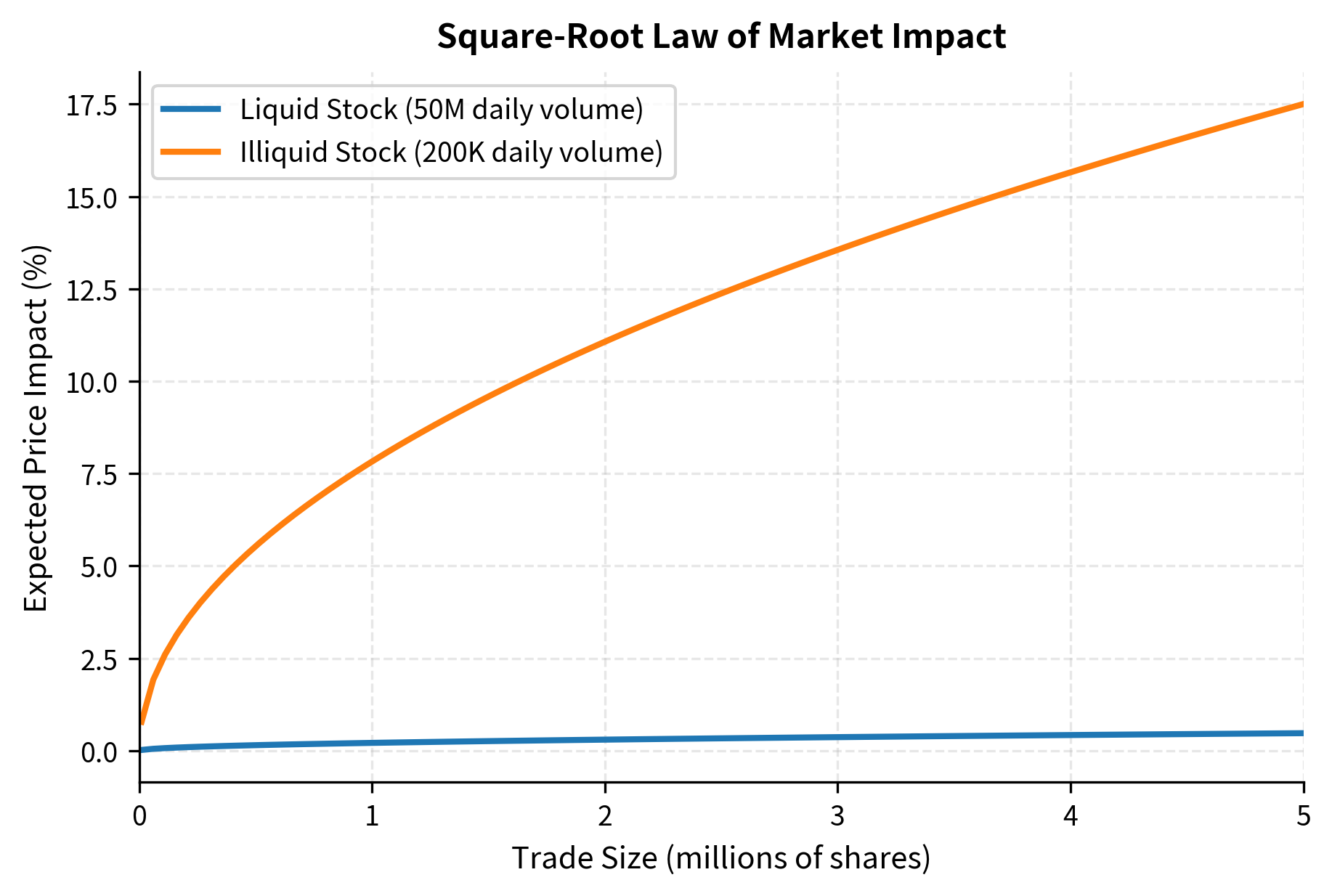
For the liquid stock, trading 1 million shares (2% of daily volume) produces an expected impact of about 0.21%. The same 1 million shares in the illiquid stock represents 500% of daily volume and would generate impact exceeding 7%, if such a trade could even be executed without moving the market further.

The practical implication of the square-root law is that optimal trade execution requires patience. Because impact grows with the square root of trade size, splitting a large order into smaller pieces and executing over time typically reduces total impact cost. If you can spread your trading over four days instead of one, the impact per day falls, and the sum of four days of smaller impacts is less than the single-day impact of trading all at once. This insight underlies the extensive literature on optimal execution algorithms that balance urgency against market impact.

While market liquidity concerns the ability to transact in asset markets, funding liquidity addresses a different question: can you meet your cash obligations as they come due? Funding liquidity risk emerges when you cannot raise cash through normal channels, such as borrowing, selling assets, or collecting receivables, at reasonable cost.

The distinction between market liquidity and funding liquidity is subtle but crucial. Market liquidity is about the ability to transform assets into cash at fair value. Funding liquidity is about the ability to obtain cash when you need it, regardless of the source. You might have excellent market liquidity in your assets but still face a funding crisis if your creditors refuse to roll over short-term debt. Conversely, you might have ample funding from stable, long-term sources but hold illiquid assets that cannot be sold without significant losses.

The danger of funding liquidity risk lies in its self-reinforcing nature. When creditors perceive you as having funding difficulties, they become less willing to lend, which exacerbates the funding difficulties, which further reduces creditor willingness to lend. This feedback loop can transform temporary cash flow mismatches into existential crises within days or even hours.

Funding needs arise from several sources that can coincide during stress periods:

• Margin calls: As positions move against you, derivatives counterparties and prime brokers demand additional collateral. Recall from our discussion of counterparty risk in Chapter 5 that collateral posting is a key mitigation technique, but it creates cash demands precisely when markets are most stressed.

• Debt maturities: Short-term borrowing must be rolled over regularly. If creditors become nervous about your creditworthiness, they may refuse to refinance or demand higher rates.

• Redemption requests: You face withdrawal demands from your investors. During market stress, redemption requests typically spike just as asset values decline.

• Operational cash needs: Payroll, rent, and other fixed obligations continue regardless of market conditions.

Each of these sources presents its own challenges. Margin calls are particularly problematic because they create "wrong-way risk," where the demand for cash increases precisely when your portfolio is performing poorly and your ability to generate cash is most constrained. Debt maturities concentrate refinancing risk at specific dates, creating calendar-based vulnerabilities. Redemptions introduce behavioral dynamics, as investors' decisions to withdraw are influenced by their beliefs about what other investors will do, potentially creating self-fulfilling runs. Operational needs establish a floor below which cash reserves cannot fall without threatening your basic functioning.

The timing correlation among these sources amplifies risk dramatically. During a market crisis, asset prices fall, triggering margin calls, which reduces the collateral available to support borrowing, which makes creditors nervous about refinancing debt, which spreads to investors who begin redeeming, all while operational needs continue unabated. The simultaneous activation of multiple funding demands is what transforms manageable cash needs into funding crises.

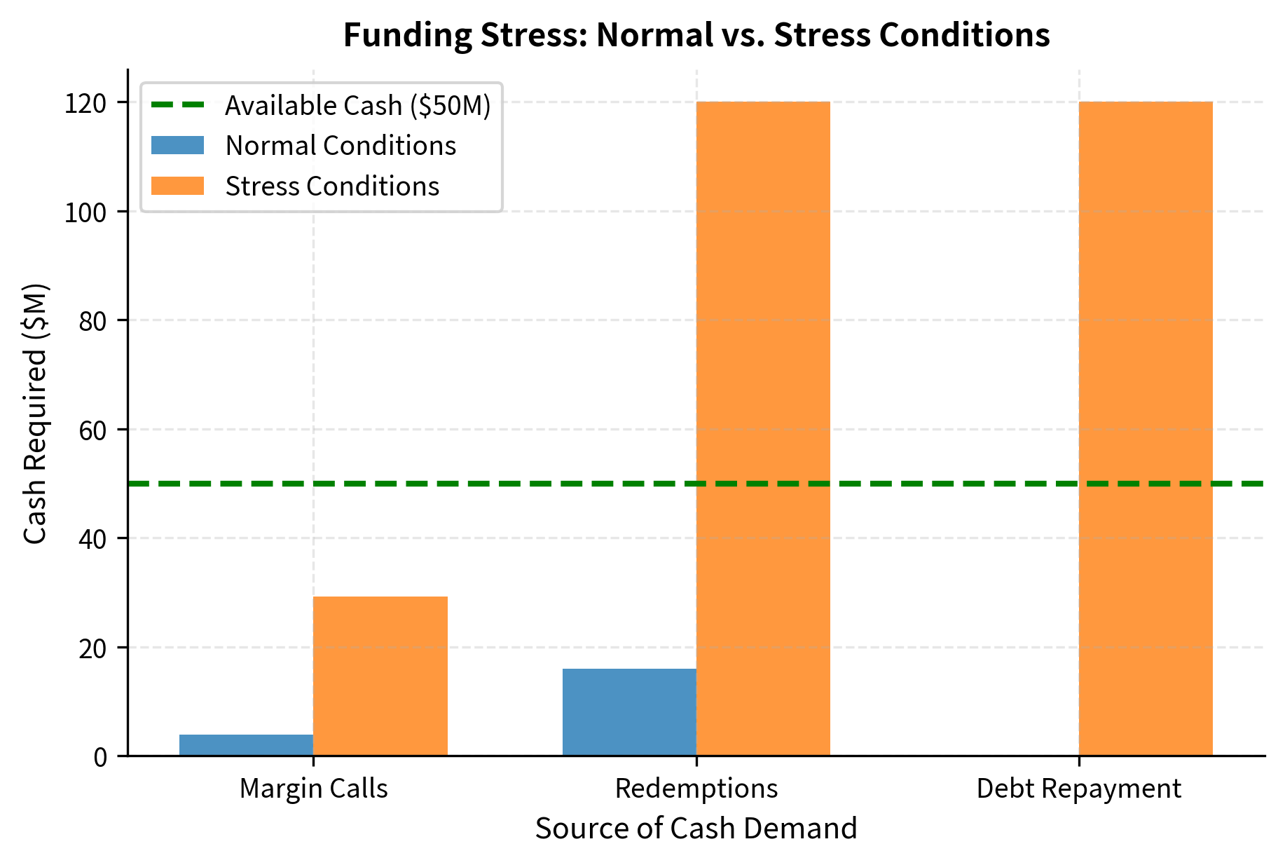
Under normal conditions, the fund's cash reserves easily cover its obligations. Under stress, the simultaneous spike in margin calls, redemptions, and debt repayment creates a shortfall exceeding 20% of assets under management. We must either sell assets, potentially at distressed prices, or default on some obligations.

The stress scenario illustrates why funding liquidity risk requires forward-looking management. Once a funding crisis materializes, options become severely constrained. Assets must be sold at whatever prices the market will bear, potentially crystallizing losses that would have been temporary if we could have weathered the storm. Counterparties who sense weakness may accelerate their demands. The premium for obtaining liquidity, whether through borrowing or asset sales, rises precisely when the need is greatest. Prudent funding risk management therefore focuses on maintaining buffers and access to funding sources before crises occur, not on scrambling to find cash when the shortfall has already materialized.

The most dangerous aspect of liquidity risk is its tendency to amplify market risk through feedback loops. When market prices decline, margin calls force you to sell if you are leveraged. Your selling pressure pushes prices lower, triggering more margin calls. This feedback mechanism can transform modest price declines into market collapses.

The mechanics of this feedback loop deserve careful examination because they explain how localized problems can become systemic crises. The loop begins with an initial price shock, perhaps from new economic information, a change in risk sentiment, or selling by a distressed institution. This initial shock reduces the equity value of your leveraged portfolios, causing your portfolios to fall below their margin requirements.

The margin mechanism then creates forced selling. If you cannot meet margin calls, you must reduce your positions to restore compliance with margin requirements. This forced selling is largely price-insensitive because you must transact regardless of market conditions. The forced selling pushes prices lower, which further reduces portfolio equity, which triggers additional margin calls, which forces more selling. The cycle continues until either prices fall far enough that forced sellers have completely liquidated, prices fall enough that value investors step in to absorb the selling pressure, or external intervention (such as central bank action) breaks the cycle.

Several factors determine how severe the feedback loop becomes. Higher leverage magnifies the effect because small price moves trigger large margin calls. Concentrated positions create greater price impact when liquidated. Correlated portfolios mean that many investors face margin calls simultaneously, overwhelming the market's capacity to absorb selling. Short liquidation horizons force rapid selling, which has greater price impact than gradual liquidation would.

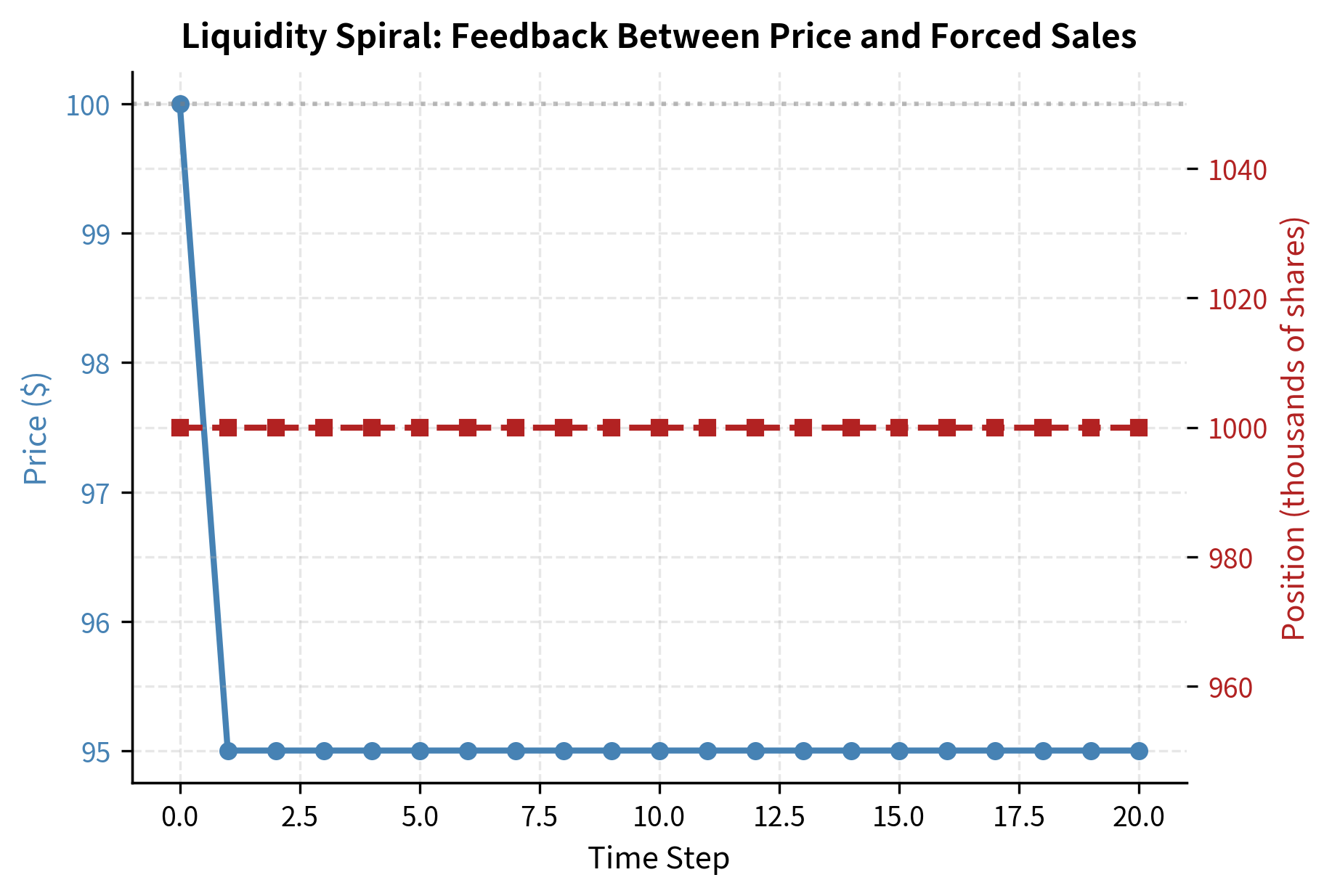
What began as a 5% price shock resulted in a much larger total loss as the feedback loop amplified the initial decline. The fund was forced to sell into falling prices, locking in losses and contributing to further price declines that affected all market participants.

The simulation demonstrates why leverage is sometimes described as a "Faustian bargain." In good times, leverage amplifies returns and allows investors to hold larger positions than their capital would otherwise permit. In bad times, the margin mechanism forces deleveraging at the worst possible moment, transforming paper losses into permanent losses and potentially propagating distress to others who hold similar positions. The feedback loop explains why financial crises often exhibit nonlinear dynamics: small triggers can produce enormous consequences once the loop begins operating.

Understanding liquidity risk requires studying its manifestations in real markets. Several historical episodes illustrate how liquidity can evaporate precisely when it is most needed.

LTCM was a hedge fund that employed highly leveraged convergence trades, betting that spreads between related securities would narrow. With $4 billion in equity supporting $125 billion in assets and off-balance-sheet derivative positions with notional values exceeding $1 trillion, LTCM's leverage ratios were extreme.

When Russia defaulted on its debt in August 1998, global investors fled to safety, widening the spreads LTCM was betting would narrow. As losses mounted, LTCM faced margin calls it could not meet. Worse, the firm's positions were so large that any attempt to unwind would devastate already-stressed markets. Other market participants, aware of LTCM's distress, pulled back liquidity precisely when LTCM needed it most.

The Federal Reserve organized a private-sector bailout, with 14 banks contributing $3.6 billion to prevent a disorderly collapse that could have triggered systemic contagion. LTCM's demise illustrated how leverage, concentrated positions, and liquidity risk can combine catastrophically.

The 2008 crisis demonstrated liquidity risk on a systemic scale. It revealed the dangers of what economists call "liquidity illusion": assets that appear liquid under normal conditions but become impossible to trade during stress.

Mortgage-backed securities and collateralized debt obligations, which had traded with reasonable spreads before the crisis, became essentially untradeable. Banks that had relied on short-term wholesale funding found creditors unwilling to roll over loans. Money market funds, considered safe havens, "broke the buck" when they could not liquidate holdings at par. The Federal Reserve and Treasury intervened with unprecedented programs to provide liquidity that private markets had withdrawn.

When redemption requests exceed available liquidity, funds may suspend redemptions entirely, a practice called "gating." During the 2008 crisis, numerous hedge funds gated investors, preventing withdrawals even as portfolio values plummeted. More recently, several UK property funds suspended redemptions in 2016 following the Brexit referendum, and multiple credit funds gated during the March 2020 COVID-19 market panic.

Gating protects remaining investors from the forced-sale losses that would occur if the fund liquidated holdings at distressed prices. However, it violates investors' liquidity expectations and can trigger panic elsewhere as investors rush to withdraw from similar funds before gates are imposed.

Unlike market risk, where VaR provides a standardized measure, liquidity risk lacks a single dominant metric. We use multiple complementary measures to assess different dimensions of liquidity.

The absence of a single liquidity measure reflects the multifaceted nature of the risk itself. Market liquidity and funding liquidity are distinct phenomena. Liquidity varies across time, across assets, and across market conditions. What matters is not just current liquidity but how liquidity might change under stress. These complexities require a portfolio of metrics rather than a single summary statistic.

The simplest liquidity measures are based on bid-ask spreads. These measures capture the immediate cost of transacting and provide a first-order approximation of market liquidity:

• Absolute spread: Best ask minus best bid
• Relative spread: Spread divided by mid-price (percentage cost)
• Effective spread: The actual cost of execution, which may differ from quoted spreads due to price improvement or slippage

The absolute spread tells you the dollar cost per share of crossing from bid to ask. The relative spread normalizes this cost as a percentage of the asset price, allowing comparison across assets with different price levels. A $0.10 spread on a $10 stock (1%) is very different from a $0.10 spread on a $100 stock (0.1%), and the relative spread captures this distinction.

The effective spread deserves special attention because it measures what traders actually experience rather than what the order book displays at a moment in time. Trades may execute inside the quoted spread if a market maker offers price improvement, or outside the spread if the order is large enough to consume multiple price levels. By comparing actual execution prices to the contemporaneous mid-price, the effective spread reveals true transaction costs.

Volume metrics capture how easily large positions can be traded. While spread-based measures focus on the cost of small transactions, volume-based measures address the capacity dimension of liquidity:

• Average daily volume (ADV): The typical trading volume over a period
• Days to liquidate: Position size divided by a sustainable daily trading rate (typically 10-25% of ADV)
• Participation rate: Your trading volume as a fraction of total market volume

Average daily volume establishes a benchmark for what the market normally absorbs. Trading significantly more than average volume signals to the market that something unusual is occurring and typically triggers adverse price movements. The "days to liquidate" metric translates position sizes into time, revealing how long it would take to exit a position at a sustainable pace.

The participation rate, sometimes called the "footprint," measures how visible your trading is to other market participants. A 5% participation rate means you are contributing one of every twenty trades; you are present but not dominant. A 50% participation rate means you are half of all market activity; you cannot hide, and other participants will adjust their behavior in response to your presence. High participation rates both increase price impact and expose you to predatory trading from others who recognize your need to transact.

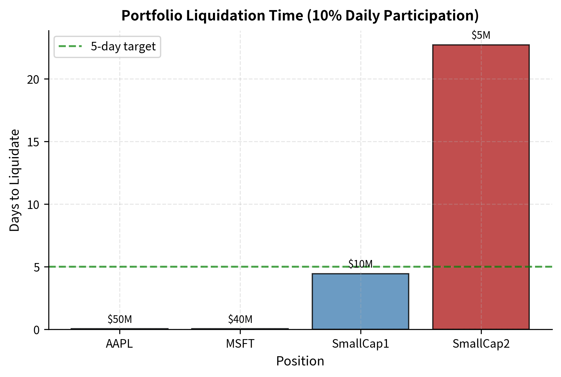
Even though the small-cap positions represent a small fraction of portfolio value, they create a liquidity bottleneck. The entire portfolio cannot be liquidated faster than the least liquid position allows. This is a critical consideration for funds that may face redemption pressure.

The bottleneck effect has important implications for portfolio construction. A portfolio might have an average liquidity profile that appears acceptable, yet contain positions that would take weeks or months to exit. During a redemption event, investors request cash, not proportional slices of each position. If the liquid positions are sold first to meet redemptions, the remaining portfolio becomes increasingly illiquid, potentially trapping remaining investors in positions they cannot exit. Understanding the liquidity distribution across the portfolio, not just the average, is essential for managing this risk.

Standard VaR assumes positions can be liquidated instantaneously at current market prices. Liquidity-adjusted VaR incorporates the time and cost required to actually exit positions.

The gap between standard VaR and the reality of trading in markets represents a significant model risk. VaR answers the question: "How much could you lose if prices move against you over some horizon?" But this question implicitly assumes you can exit at those prices. In reality, the process of exiting, especially in stressed markets when others are also trying to exit, will incur additional costs. LVaR attempts to capture these costs within the VaR framework.

The simplest LVaR adjustment adds the expected liquidation cost to the standard VaR:

where:

• LVaR: Liquidity-adjusted Value at Risk
• VaR: standard Value at Risk (market risk)
• Liquidation Cost: estimated cost to close the position, accounting for spread, price impact, and time to liquidate

This additive approach treats liquidity cost as deterministic, which is a simplification. In reality, liquidity costs are uncertain and often correlate with market stress: spreads widen, market depth evaporates, and price impact increases precisely when VaR losses are being realized. More sophisticated LVaR approaches model the joint distribution of market returns and liquidity costs, recognizing that the worst market losses often coincide with the worst liquidity conditions.

The components of liquidation cost each capture a distinct friction. The spread cost reflects the immediate penalty of crossing the bid-ask spread to execute. The market impact cost reflects the price movement caused by the trade itself. The extended holding risk captures the additional market risk incurred when positions cannot be liquidated within the standard VaR horizon. For illiquid positions that take days or weeks to exit, this extended holding period substantially increases risk exposure.

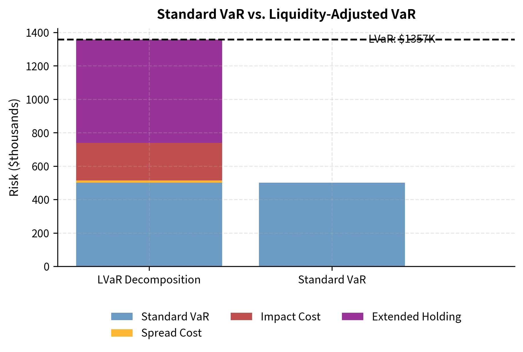
The liquidity adjustment nearly doubles the risk estimate in this example. For portfolios with significant illiquid holdings, the gap between standard VaR and LVaR can be even larger, revealing hidden risks that standard measures miss.

This substantial adjustment illustrates why liquidity risk cannot be treated as a footnote to market risk. For this position, ignoring liquidity risk would understate true risk exposure by nearly half. Risk managers who rely solely on standard VaR may believe they are operating with comfortable risk buffers when in fact their true exposure is much larger. The difference between VaR and LVaR represents a form of "liquidity illusion" that can prove fatal during market stress.

The key parameters for Liquidity-Adjusted VaR (LVaR) are:

• Standard VaR: The baseline market risk measure assuming instantaneous liquidation. This captures the risk from adverse price movements over the VaR horizon and serves as the foundation upon which liquidity adjustments are built.
• Position Value: The total market value of the position to be liquidated. Larger positions face greater liquidity challenges because they require more market capacity to absorb.
• Spread: The bid-ask spread expressed as a percentage. This represents the immediate cost of crossing the spread. In LVaR calculations, typically half the spread is used since you only pay one side when exiting.
• Days to Liquidate: The estimated time required to exit the position without excessive price impact. This is determined by position size, average daily volume, and the maximum acceptable participation rate. Longer liquidation periods increase both the time component of risk and the accumulated impact cost.
• Daily Volatility: The volatility of the asset, used to estimate price impact and risk over the extended liquidation horizon. Higher volatility increases both the expected impact (since impact scales with volatility in the square-root law) and the risk of adverse price movements during the liquidation period.

These parameters interact in important ways. Higher volatility increases both the standard VaR component and the liquidity adjustment. Longer liquidation periods compound the effect of volatility through the square-root scaling of both impact and extended holding risk. Wider spreads are often correlated with longer liquidation times, since illiquid assets typically have both wider spreads and lower trading volumes. Understanding these interactions is essential for properly calibrating LVaR models.

Effective liquidity risk management combines quantitative limits with operational controls and behavioral considerations.

A straightforward approach limits position sizes as a fraction of average trading volume. This ensures you can liquidate positions within acceptable timeframes without excessive market impact.

The logic behind volume-based limits is straightforward. If you want to be able to exit any position within, say, five days at a participation rate of 15% of daily volume, then your maximum position size is five times 15%, or 75% of average daily volume. This calculation can be inverted: given a position size and volume data, compute how long liquidation would take at a prudent participation rate. If the answer exceeds what you can tolerate given your funding structure and redemption terms, the position is too large.

These limits should reflect your specific circumstances. If you have locked-up capital and no leverage, you can tolerate longer liquidation horizons than if you face daily redemptions and margin calls. A proprietary trading desk with minimal external funding pressure has more flexibility than you would as an asset manager meeting client redemptions. The limits should be calibrated to the worst plausible funding scenario, not to normal conditions.

The small-cap positions substantially exceed their liquidity-based limits. We would require these positions to be reduced or require special approval documenting why the liquidity risk is acceptable.

The limit breaches in the small-cap positions highlight a common tension in portfolio management. Small-cap stocks often offer attractive return opportunities precisely because their illiquidity deters other investors. The same illiquidity that creates the opportunity also creates risk. Capturing this opportunity while managing the risk requires explicit acknowledgment of the liquidity constraints and appropriate position sizing. Limits provide the framework for this balancing act.

Beyond position limits, institutions maintain explicit liquidity buffers: cash reserves, credit lines, and unencumbered high-quality liquid assets that can be converted to cash quickly during stress.

The purpose of a liquidity buffer is to provide time. When funding pressure arrives, the buffer absorbs the initial shock, buying time to execute an orderly liquidation of less liquid assets, renegotiate with creditors, or wait for market conditions to improve. Without a buffer, any funding shortfall must be met by immediate asset sales, likely at distressed prices.

The size of the buffer should reflect your funding profile. Key questions include: What is the maximum plausible cash need in a stress scenario? How quickly could that need materialize? What sources of cash would be available? How long would it take to liquidate assets? The buffer should be sufficient to bridge the gap between the arrival of cash needs and the availability of cash from asset sales or alternative funding sources.

Key components of a liquidity buffer include:

• Cash and cash equivalents: Immediately available for margin calls or redemptions
• High-quality liquid assets (HQLA): Government bonds and other securities that can be sold quickly with minimal price impact
• Committed credit facilities: Pre-arranged borrowing capacity that can be drawn during stress
• Repo capacity: Ability to borrow against securities holdings

Banks operating under Basel III regulations must maintain a Liquidity Coverage Ratio (LCR) ensuring you hold sufficient HQLA to cover 30 days of stressed cash outflows:

where:

• LCR: Liquidity Coverage Ratio
• High-Quality Liquid Assets: unencumbered high-quality liquid assets (HQLA)
• Total Net Cash Outflows over 30 days: total expected cash outflows minus total expected cash inflows over the next 30 calendar days

The LCR formula embodies a principle that extends beyond banking regulation. The numerator represents your resources: what you can convert to cash quickly. The denominator represents your requirements: what you might need to pay in a stressed scenario. Maintaining a ratio above 100% ensures you can meet stressed outflows from your liquid reserves alone, without relying on asset sales or new funding that might not be available during stress.

Operational risk encompasses losses arising from inadequate or failed internal processes, people, and systems, or from external events. Unlike market or credit risk, operational risk does not arise from taking positions. It stems from the operational infrastructure that supports all financial activities.

Operational risk is often described as "everything that is not market or credit risk," which hints at both its pervasiveness and its heterogeneity. Every transaction requires operational execution: trades must be entered correctly, settlements must occur on time, accounts must be reconciled, systems must function, and people must perform their roles competently. Each of these activities presents opportunities for error, fraud, or failure.

Operational risk manifests through diverse failure modes:

• Internal fraud: Unauthorized trading, theft, falsified records. Nick Leeson's unauthorized trades that destroyed Barings Bank and the London Whale's concealed losses at JPMorgan Chase both represent internal fraud that evaded risk controls.

• External fraud: Cyber attacks, customer fraud, forgery. Financial institutions face constant attempts at unauthorized access, phishing, and transaction manipulation.

• Employment practices: Discrimination claims, workplace safety, labor disputes. These create legal liability and operational disruption.

• Business disruptions: Technology failures, power outages, natural disasters. The 9/11 attacks destroyed critical infrastructure and forced firms to activate business continuity plans.

• Execution failures: Settlement errors, accounting mistakes, miscommunication with counterparties. Even small execution errors can compound into significant losses.

Operational risk is notoriously difficult to quantify because operational failures are rare, varied, and often reflect unique circumstances. Nevertheless, regulators require banks to hold capital against operational risk, and institutions have developed several approaches.

The fundamental challenge in quantifying operational risk is that the most important events are the rarest and most varied. Market risk can be estimated from daily returns: we have thousands of observations and can fit statistical distributions. Credit risk benefits from large portfolios: even if individual defaults are rare, a bank with thousands of loans can observe enough defaults to estimate default rates. Operational risk offers neither advantage. Major operational failures occur infrequently, each event is often unique in its details, and the most severe losses often stem from scenarios that had never previously occurred.

This data scarcity creates a modeling paradox. The loss events we most need to understand, meaning the extreme events that threaten institutional solvency, are precisely the events for which we have the least data. Any distribution fitted to operational loss data will be heavily influenced by the one or two largest historical losses, making the resulting capital estimate highly sensitive to accidents of history.

The Basic Indicator Approach under Basel regulations sets operational risk capital as a fixed percentage of gross income:

where:

• OpRisk Capital: regulatory capital charge for operational risk
• \alpha: fixed percentage factor (typically 15%)
• Average Gross Income: average annual gross income over the preceding three years

This simple approach requires no loss modeling but provides no discrimination between institutions with strong versus weak operational controls.

The appeal of the Basic Indicator Approach lies in its simplicity and objectivity. Gross income is readily available from financial statements, and the calculation is straightforward. However, the approach implicitly assumes that operational risk scales linearly with business volume and that all institutions face similar operational risk per dollar of revenue. Neither assumption is particularly accurate. A well-controlled firm may have lower operational risk than a poorly controlled one of the same size. Certain business lines may have inherently higher operational risk than others. The Basic Indicator Approach ignores these distinctions.

More sophisticated approaches use internal loss data, external loss databases, scenario analysis, and business environment factors to estimate operational risk distributions. However, the heavy-tailed nature of operational losses, where a single event can dwarf years of routine losses, makes distribution fitting challenging.

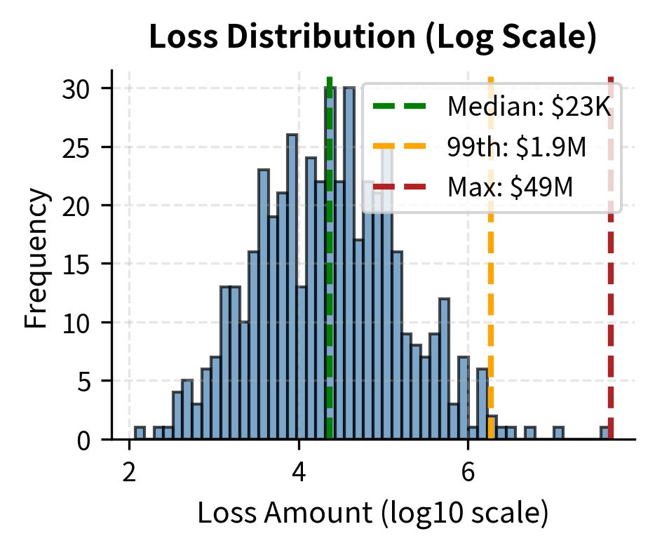
The simulation illustrates the heavy-tailed nature of operational risk: the maximum single loss is many times larger than the typical event. This characteristic makes operational risk capital calculations highly sensitive to assumptions about tail behavior.

The enormous ratio between the maximum loss and the median event captures a fundamental truth about operational risk: the typical event is nearly irrelevant for capital purposes. A firm might experience fifty small operational losses per year, each costing tens of thousands of dollars. These are annoying but manageable. The danger lies in the rare event that costs millions or billions, potentially threatening the firm's existence. Operational risk management must therefore focus disproportionately on preventing catastrophic failures, not on reducing the frequency of routine errors.

Model risk is the risk of loss arising from decisions based on incorrect or misused models. In quantitative finance, where models drive trading, hedging, pricing, and risk management decisions, model risk is both pervasive and potentially catastrophic.

Models occupy a peculiar position in finance. They are indispensable tools for understanding complex instruments and market dynamics, yet they are also systematic sources of error. Every model simplifies reality, and every simplification carries the risk that some omitted factor will prove important. The danger is magnified by the confidence that quantitative methods can inspire: a precise numerical output may appear more reliable than it actually is, leading you to underestimate the uncertainty inherent in model-based analysis.

Model risk emerges from several distinct failure modes:

Incorrect model specification occurs when the model's mathematical structure fails to capture the true data-generating process. The Black-Scholes model assumes constant volatility, but as we discussed in the chapter on implied volatility and the volatility smile, this assumption is violated empirically. Using Black-Scholes for exotic options or during volatility regimes different from those assumed can produce systematically biased prices.

The challenge with specification error is that it can be invisible in normal times yet catastrophic in stress. A model calibrated to benign market conditions may fit historical data well, pass backtests, and produce reasonable-looking outputs for an extended period. The flaws only become apparent when conditions shift beyond the model's domain of validity. By then, positions may have been sized based on the model's optimistic risk estimates, and the true risks may be far larger than believed.

Calibration errors arise when model parameters are estimated incorrectly or from inappropriate data. A volatility estimate calibrated to a calm period will understate risk during turbulent markets. The Gaussian copula models used for CDO pricing, which we covered in the chapter on structured credit products, were often calibrated to short historical periods that did not include credit stress, leading to dramatic underestimation of correlation risk.

Calibration error highlights the importance of the data used to estimate model parameters. Parameters estimated from two years of data may not reflect the dynamics that emerge over longer cycles. Parameters estimated from one market regime may not apply in another. The model may be mathematically correct but rendered dangerous by parameters that do not reflect current or future conditions.

Implementation errors occur when the mathematical model is translated incorrectly into code. A misplaced decimal point, incorrect sign, or boundary condition error can cause a correctly specified model to produce wrong outputs. Such bugs may go undetected for extended periods if results appear plausible.

Implementation errors are insidious because they can produce outputs that look reasonable superficially. A pricing model with a sign error might produce prices that are in the right general range, pass cursory sanity checks, and only reveal the problem through systematic P&L discrepancies that accumulate over time. The more complex the model, the more opportunities for implementation error and the harder the error is to detect.

Inappropriate application happens when a model designed for one purpose is used for another. A model calibrated for liquid exchange-traded options may perform poorly for illiquid over-the-counter structures. Using overnight VaR for positions that take weeks to liquidate understates risk.

Every model has a domain of applicability: the conditions under which its assumptions approximately hold and its outputs can be trusted. Using a model outside its domain is a form of model risk that arises from your behavior rather than model construction. It often reflects organizational pressures: a model exists and produces a number, so the number gets used even when the model is not appropriate for the situation at hand.

The London Whale episode at JPMorgan Chase in 2012 illustrates how model risk can enable massive losses. The bank's Chief Investment Office had accumulated large positions in credit derivatives. When the positions moved against the bank, the risk models used by the CIO, which differed from those used by the bank's central risk function, showed lower VaR than alternative approaches would have indicated.

The CIO's VaR model was modified mid-crisis in ways that reduced reported risk, masking the true exposure. By the time the positions were unwound, losses exceeded $6 billion. The incident revealed failures in model governance, approval processes, and the independence of model validation from business units that benefited from favorable model outputs.

The London Whale case illustrates several model risk pathologies. The business unit had latitude to choose its own risk model, creating an incentive to select or modify the model to produce favorable numbers. Model changes were made during a period of stress without adequate scrutiny. The disconnect between the CIO's reported risk and the central risk function's assessment was not escalated effectively. Each of these failures represents a breakdown in model risk governance that allowed the model to become a tool for concealing rather than revealing risk.

Robust model risk management requires multiple layers of defense:

Independent model validation ensures models are reviewed by teams separate from those who build or use them. Validators test model assumptions, check implementations, and assess model performance against out-of-sample data.

The independence of validation is crucial because those who build or use models have incentives that may not align with accurate risk assessment. Traders want models that support their positions. Structurers want models that help sell products. Risk managers who built a model may be reluctant to acknowledge its flaws. Independent validators, with no stake in the model's outputs, can provide objective assessment.

Model inventory and tiering documents all models in use and classifies them by materiality. Higher-tier models receive more intensive validation and oversight.

Not all models warrant the same attention. A model used to price a single small position should not require the same validation effort as a model used to price a large and complex portfolio. Tiering ensures that validation resources are allocated according to the potential impact of model failure.

Ongoing monitoring tracks model performance over time. When model predictions diverge systematically from realized outcomes, the model may require recalibration or replacement.

Models can degrade over time even without any change to their structure. Market dynamics evolve, parameter estimates become stale, and relationships that held historically may break down. Ongoing monitoring detects this degradation before it causes significant losses.

Limitations documentation explicitly records known model limitations and the conditions under which the model may perform poorly. You must understand these limitations before relying on model outputs.

Every model has limitations, and hiding those limitations creates risk. Explicit documentation forces acknowledgment of what the model cannot do and alerts users to conditions where extra caution is warranted.

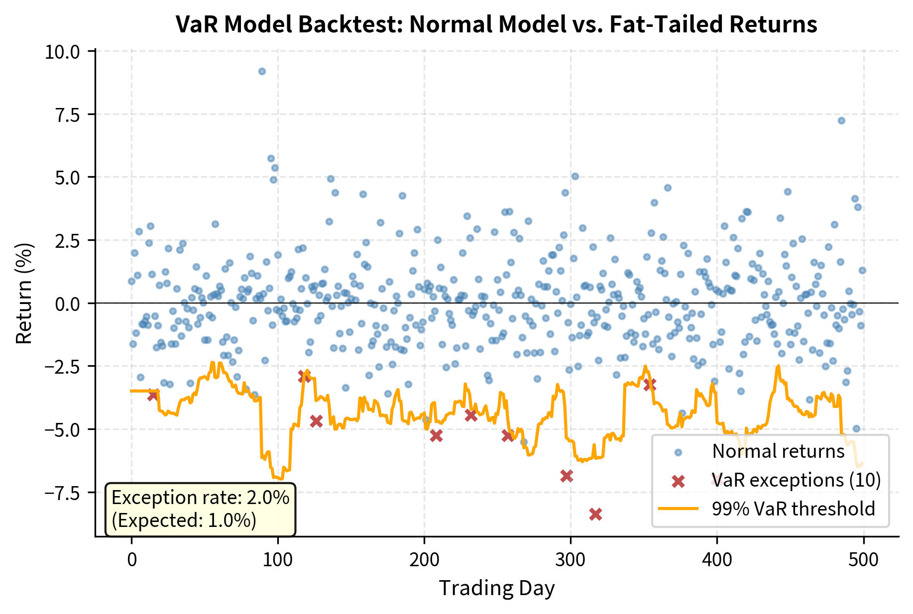
The normal distribution-based VaR model underestimates tail risk when true returns have fat tails. The backtest reveals more exceptions than expected, indicating the model needs revision. Such backtesting is essential for ongoing model validation.

The backtest results demonstrate how specification error manifests in practice. The normal distribution assumption underestimates the probability of extreme returns, causing VaR to be exceeded more often than the model predicts. The ratio of actual to expected exceptions quantifies the degree of underestimation. A ratio significantly above one is a warning sign that should trigger model review.

Not all risks can be reduced to numbers. Effective risk management requires qualitative assessment alongside quantitative measures, particularly for risks that are rare, complex, or poorly understood.

Scenario analysis explores how portfolios and institutions would perform under specific hypothetical or historical stress conditions. Unlike VaR, which provides a statistical summary, scenarios tell stories: what if interest rates rise 300 basis points while credit spreads widen and equity markets fall 30%? What if a major counterparty fails? What if our primary clearing bank experiences operational disruption?

The value of scenario analysis lies not in precise probability estimates (extreme scenarios are inherently difficult to assign probabilities) but in revealing vulnerabilities and stimulating contingency planning. A scenario revealing that the firm could not meet margin calls in a particular stress environment should prompt action regardless of whether that scenario has a 1% or 0.1% probability.

Quantitative models are built on explicit assumptions, but the choice of which risks to model and how to model them requires expert judgment. Risk identification workshops, control self-assessments, and structured interviews with business unit managers help surface risks that may not appear in historical data or standard risk categories.

Questions to probe include:

• What has changed since our risk models were last calibrated?
• What new products, markets, or strategies have we entered?
• What near-misses or small losses occurred that could have been much worse?
• What are our key dependencies on third parties, technology, or specific individuals?
• What is different about the current environment compared to historical stress periods?

Ultimately, risk management effectiveness depends on organizational culture and incentives. A firm where risk managers are respected, where concerns can be raised without retaliation, and where compensation structures don't reward excessive risk-taking will manage risks better than one where risk management is seen as a bureaucratic obstacle to profit.

Regulators increasingly focus on risk culture, recognizing that no amount of quantitative sophistication can substitute for an organization where people at all levels understand and respect risk limits. The failures that led to major losses, from Barings to Enron to the mortgage crisis, typically involved cultural factors: pressure to meet targets, dismissal of warnings, and incentive structures that rewarded short-term profits over long-term stability.

The most effective risk management frameworks integrate quantitative measures with qualitative assessments, recognizing the strengths and limitations of each approach.

The dashboard presents quantitative risk measures alongside qualitative concerns, preventing false precision while maintaining rigor. The model risk buffer acknowledges uncertainty in quantitative estimates, while the qualitative assessment ensures human judgment informs decision-making.

This chapter has explored the risks that operate beyond traditional market risk measures, revealing vulnerabilities that quantitative models often miss.

Market liquidity risk arises from the inability to transact without significant price impact. Bid-ask spreads, market depth, and the square-root law of market impact provide frameworks for understanding and measuring liquidity costs. Position limits based on average daily volume help ensure portfolios can be liquidated within acceptable timeframes.

Funding liquidity risk concerns the ability to meet cash obligations. Margin calls, redemptions, and debt rollovers can create simultaneous cash demands precisely when asset markets are stressed. The feedback loop between funding and market liquidity can transform modest market declines into full-scale crises, as demonstrated during LTCM's collapse and the 2008 financial crisis.

Operational risk encompasses losses from process failures, human error, systems breakdowns, and external events. While difficult to quantify due to the heterogeneous and heavy-tailed nature of operational losses, frameworks exist for estimating operational risk capital and, more importantly, for identifying and mitigating operational vulnerabilities.

Model risk emerges from the quantitative frameworks we use to measure other risks. Incorrect specifications, calibration errors, implementation bugs, and inappropriate applications can cause models to fail precisely when they are most needed. Independent validation, ongoing backtesting, and explicit documentation of model limitations provide defenses against model risk.

Qualitative assessment complements quantitative measures for risks that resist easy quantification. Scenario analysis explores vulnerabilities that historical data may not reveal. Expert judgment identifies emerging risks before they appear in loss data. Risk culture ensures that organizational incentives align with prudent risk-taking.

The next chapter examines how these risk measures and assessments are integrated into coherent risk management policies and practices at the institutional level, addressing governance structures, limit frameworks, and the practical challenges of implementing risk management in complex organizations.

Ready to test your understanding? Take this quick quiz to reinforce what you've learned about liquidity risk and other non-market risks.