

Master Credit Valuation Adjustment for derivatives pricing. Learn exposure profiles, default probability modeling, and the complete XVA framework.
Choose your expertise level to adjust how many terms are explained. Beginners see more tooltips, experts see fewer to maintain reading flow. Hover over underlined terms for instant definitions.
Counterparty Risk and CVA
When you enter into a derivative contract with another party, you face a risk that goes beyond market movements: the risk that your counterparty might default before fulfilling their obligations. This counterparty credit risk became painfully apparent during the 2008 financial crisis when the collapse of Lehman Brothers left thousands of derivative counterparties with enormous unexpected losses. The event transformed how financial institutions think about and price derivatives, leading to a fundamental shift in valuation practices.
Credit Valuation Adjustment (CVA) emerged as the industry standard for quantifying this risk. Unlike traditional credit risk on loans where the exposure is the principal amount, derivative exposures fluctuate with market conditions and can swing from positive to negative over the contract's life. This creates a unique challenge: you need to project future exposure profiles, estimate default probabilities, and integrate these over time to arrive at a fair price for counterparty risk.
In this chapter, we develop the theoretical framework for measuring counterparty risk and calculating CVA. We build exposure profiles using simulation techniques from Part III, connect default probabilities to CDS spreads as covered in Chapter 13 of Part II, and implement practical CVA calculations. We also examine how CVA desks manage this risk and briefly introduce the broader family of valuation adjustments that modern derivatives pricing requires.
Counterparty Credit Risk Fundamentals
Counterparty credit risk is the risk that the counterparty to a financial transaction will default before the final settlement of the transaction's cash flows. To understand why this risk requires special treatment, we must recognize how it differs fundamentally from the credit risk encountered in traditional lending. When a bank makes a loan, the exposure is straightforward: the lender has a fixed claim on the borrower for the principal and interest owed. The borrower, by contrast, has no corresponding credit exposure to the bank. In derivative contracts, however, the situation is far more complex, and several distinguishing characteristics emerge:
- Bilateral exposure: Unlike a loan where only the lender faces risk, derivative contracts can have positive or negative value for either party, creating two-way risk
- Time-varying exposure: The amount at risk changes throughout the contract's life as market conditions evolve
- Netting and collateral: Legal agreements can reduce exposure through netting sets and margin posting.
These characteristics mean that counterparty credit risk cannot be measured with a single number determined at contract inception. Instead, we must develop dynamic measures that capture how exposure evolves through time and across different market scenarios. This fundamental insight drives everything that follows in our treatment of CVA.
Counterparty credit risk covers default before settlement, while settlement risk (also called Herstatt risk) addresses the risk of default during the settlement process itself, when one party has already delivered but the other has not yet paid.
When Counterparty Risk Materializes
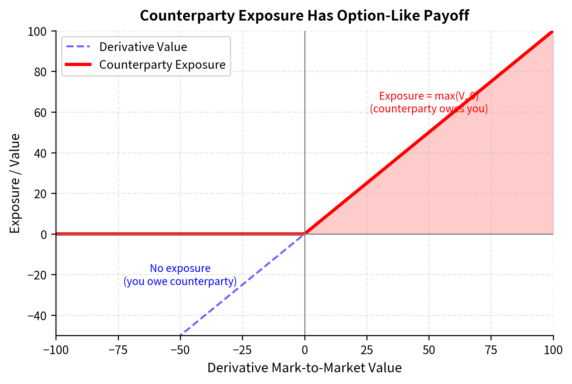
A key insight, one that shapes the entire mathematical framework for CVA, is that counterparty default only creates a loss when the derivative has positive value to you at the time of default. This observation may seem obvious at first, but its implications are significant. If your counterparty defaults when you owe them money, you actually benefit (though this raises its own accounting questions we address later with DVA). This asymmetry means counterparty risk has an option-like character: you lose if the contract is in your favor when default occurs.
To develop intuition for this asymmetry, consider what happens economically when a counterparty defaults. In most jurisdictions, derivative contracts are terminated upon default, and the non-defaulting party has a claim against the defaulting party's estate for the contract's mark-to-market value if positive. If the contract has negative value to you (meaning you owe the counterparty money), you still owe that amount to the bankruptcy estate. You do not get to walk away from your obligations simply because the other party has defaulted.
Consider an interest rate swap where you pay fixed and receive floating. If rates rise significantly, the swap becomes valuable to you; your counterparty owes you net payments. If they default in this state, you lose that value. Conversely, if rates fall, you owe them money, and their default doesn't harm you directly. This one-sided nature of the loss, where you are exposed only when the derivative has positive value, is mathematically equivalent to holding an option. Specifically, your loss upon counterparty default is the positive part of the derivative's value, which we can write as . This is the payoff of a call option on the derivative value with a strike price of zero.
Exposure Metrics
To quantify counterparty risk in a precise and actionable way, we need carefully defined metrics that capture different aspects of the exposure. Building on the credit risk concepts from Chapter 3, we introduce derivative-specific exposure measures. Each metric answers a different question that risk managers and regulators care about, and together they provide a complete picture of the counterparty risk profile.
-
Current Exposure (CE): The current mark-to-market value of the derivative if positive, zero otherwise. This represents what you would lose if default happened right now.
-
Potential Future Exposure (PFE): A high-confidence estimate (typically 95% or 99%) of exposure at a future date. This captures the potential growth in exposure due to market movements.
-
Expected Exposure (EE): The average exposure at a future date, considering all possible market scenarios weighted by their probabilities.
-
Expected Positive Exposure (EPE): The time-weighted average of expected exposures over the contract's life. Regulators often use this for capital calculations.
Let us examine each of these metrics in greater detail to understand what they measure and why each is useful. Current Exposure tells us the immediate loss we would suffer if default occurred right now. It is directly observable from today's mark-to-market value and requires no simulation or forecasting. However, current exposure alone is insufficient for risk management because it tells us nothing about how exposure might evolve in the future.
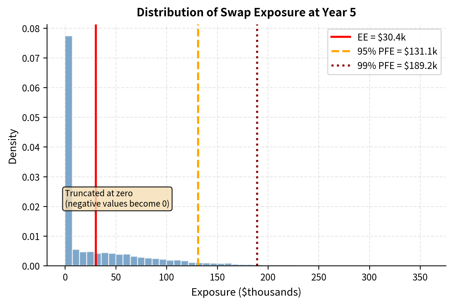
Potential Future Exposure addresses this limitation by providing a worst-case measure at each future date. When you say the PFE at year three is $5 million at the 99th percentile, you mean that in 99% of simulated scenarios, the exposure at year three is below $5 million. This metric is particularly useful for setting credit limits, as it captures tail risk rather than average outcomes.
Expected Exposure, by contrast, provides the average outcome across all scenarios. This is the appropriate measure for pricing counterparty risk because, from an expected value perspective, we should charge for the average loss rather than the worst-case loss. Expected Exposure forms the foundation of the CVA calculation we develop in subsequent sections.
Mathematically, if represents the derivative's mark-to-market value at time , the exposure metrics are defined as:
where:
- : current exposure at time , representing immediate loss upon default
- : expected exposure at time , averaging across all market scenarios
- : expected positive exposure, the time-weighted average over the contract life
- : mark-to-market value of the derivative at time
- : expectation operator under the risk-neutral measure
- : total life of the contract
The expected value is taken under the risk-neutral measure, consistent with the derivative pricing framework from Part III, Chapter 4. This choice ensures that our CVA calculation is consistent with the broader derivatives pricing methodology. Under the risk-neutral measure, we use risk-free rates for discounting, and the drift of underlying assets equals the risk-free rate minus any dividend yield. This framework allows CVA to be incorporated seamlessly into derivative valuations without arbitrage violations.
Exposure Profiles by Product Type
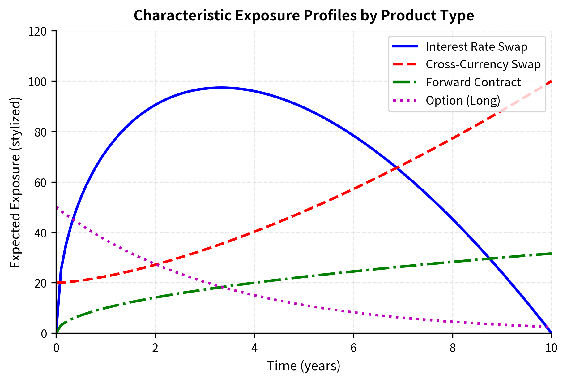
Different derivative products exhibit characteristic exposure profiles that reflect their cash flow structures. Understanding these patterns helps in CVA calculation and risk management. By examining how exposure evolves for different product types, we can develop intuition for which trades consume more counterparty credit and how to structure portfolios to manage this risk effectively.
Interest Rate Swaps
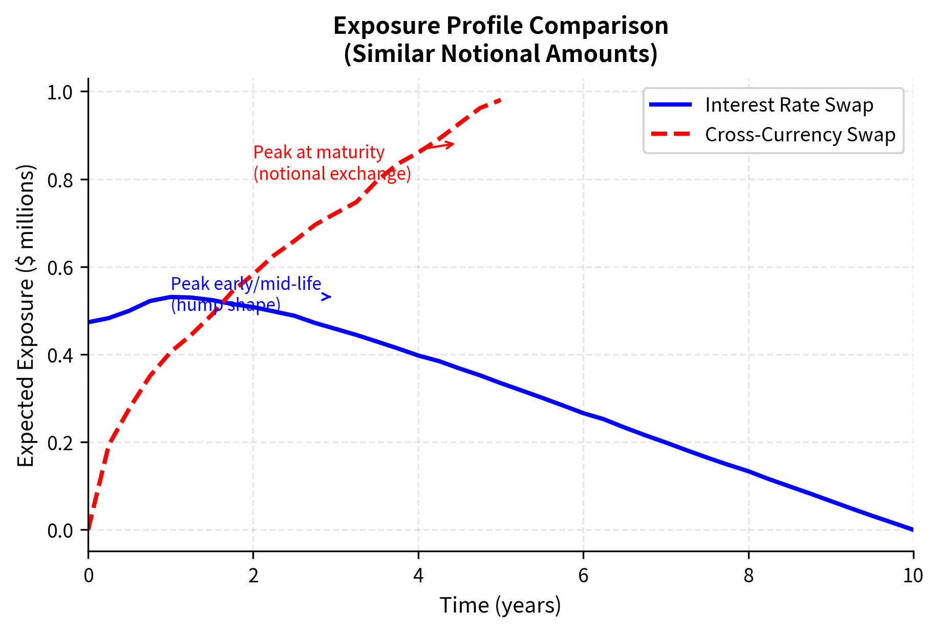
Interest rate swaps have a distinctive exposure profile that initially rises, peaks around one-third to one-half of the swap's life, then declines toward maturity. This "hump-shaped" profile arises because two opposing forces are at work:
- Early in the swap's life, there's substantial time for rates to move, creating potential exposure
- As the swap ages, fewer cash flows remain, reducing the maximum possible exposure
- Near maturity, the remaining value approaches zero regardless of rate movements
The expected exposure for a receiver swap (receive fixed, pay floating) can be approximated by considering the distribution of forward rates and their impact on the swap's present value. In the early years, rates have not had much time to deviate from their initial values, so exposure is modest. As time progresses, the cumulative effect of rate movements can create significant exposure. Eventually, however, the decreasing number of remaining payments dominates, and exposure declines as the swap approaches maturity.
Options
Option exposure is more straightforward for the buyer: the maximum loss is the premium paid, which occurs if the counterparty defaults before exercise. This creates a simple, front-loaded exposure profile that declines as the option approaches expiration and the remaining time value erodes. For the seller, exposure depends on the option's current intrinsic and time value, which can be substantial for deep in-the-money options. Sold options create contingent exposure that can spike dramatically if the option moves into the money, making counterparty risk particularly important for option sellers dealing with less creditworthy counterparties.
Cross-Currency Swaps
Cross-currency swaps typically show increasing exposure profiles because they involve the exchange of notional amounts at maturity. Unlike interest rate swaps, the notional exchange creates significant exposure near the end of the contract's life, particularly if exchange rates have moved substantially. This back-loaded exposure profile presents distinct risk management challenges. The counterparty relationship must remain healthy for many years before the largest exposures materialize, and the potential for exchange rate moves over long horizons can create very large potential future exposures.
Forward Contracts
Forwards show linearly increasing exposure profiles on average, as the potential deviation between the forward price and the spot price tends to grow with time due to random walk behavior. A forward contract locks in a price for future delivery, and as time passes, the spot price can drift further from the locked-in forward price. This drift occurs in both directions with equal probability under risk-neutral pricing, but the exposure metric captures only the positive deviations, creating a steadily increasing expected exposure profile.
The CVA Formula
Credit Valuation Adjustment represents the expected loss due to counterparty default, incorporated as an adjustment to the derivative's risk-free value. The intuition behind CVA is straightforward: if there is some probability that your counterparty will default and fail to make payments owed to you, then the derivative is worth less than its risk-free value. CVA quantifies exactly how much less the derivative is worth, providing a fair price for counterparty credit risk.
To develop the CVA formula, we need to think about what happens at each possible default time. If the counterparty defaults at time , and the derivative has positive value at that moment, you will lose a fraction of that value determined by the Loss Given Default. We must consider all possible default times, weight each by its probability, and sum to find the total expected loss.
The fundamental CVA formula is:
where:
- : Loss Given Default, the fraction of exposure lost if default occurs
- : Expected Exposure at time
- : probability of default occurring in the infinitesimal interval around time
- : maturity of the contract
The formula calculates the total expected loss by integrating over the life of the contract. At any moment , the expected loss conditional on default is . We weight this by the probability that default happens exactly at that moment, and sum these potential losses across all times from 0 to .
This continuous formula captures the essence of CVA, but continuous integration is not practical for implementation. In the real world, we observe exposure at discrete time points and must work with discrete default probabilities. The continuous formula is therefore typically discretized for practical computation:
where:
- : marginal probability of default between times and
- : expected exposure at time
- : Loss Given Default
- : discrete time points where exposure is calculated
- : number of time steps in the simulation
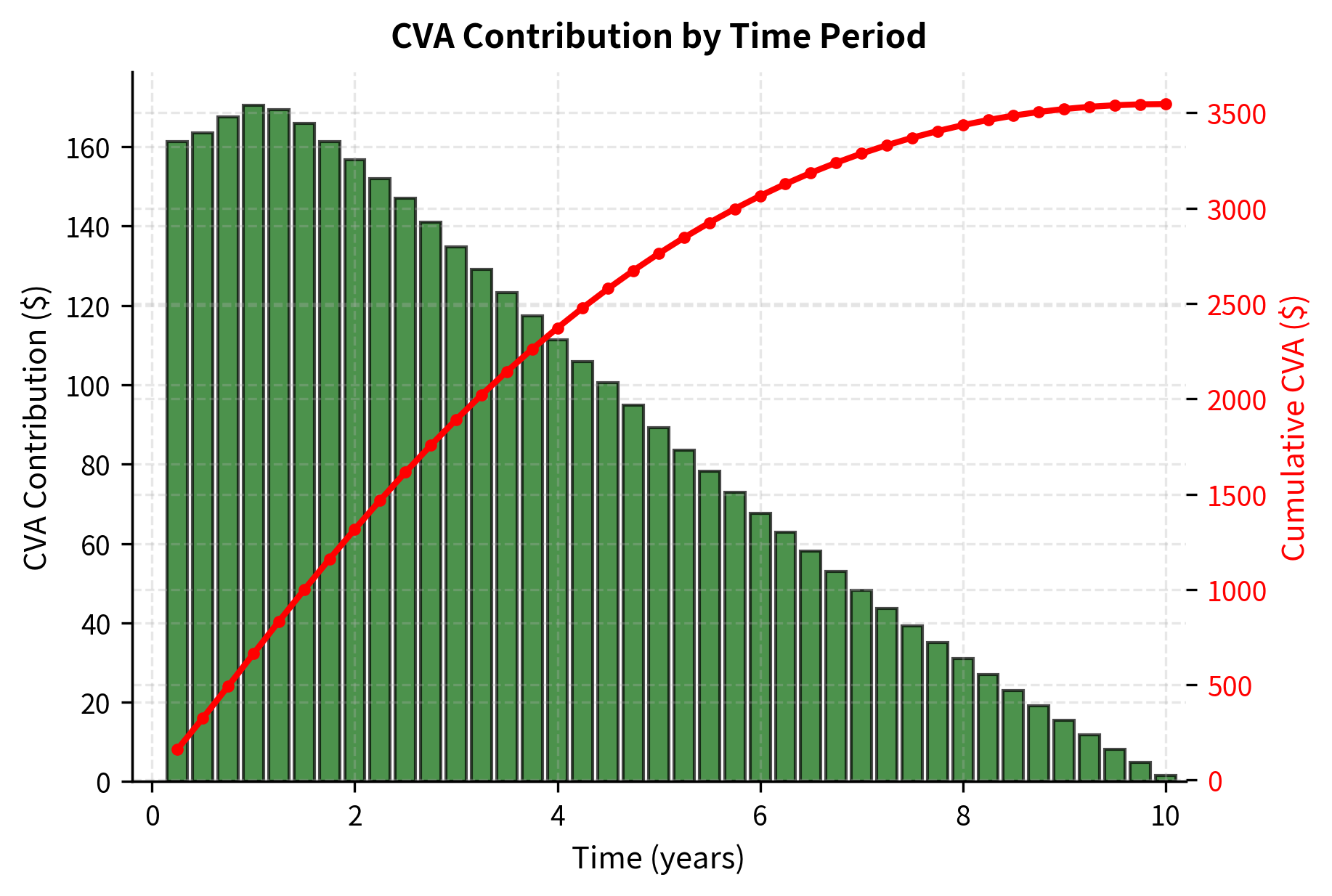
The discrete formula partitions the contract life into intervals and computes the contribution to CVA from each interval. For interval , the contribution equals the expected loss if default occurs in that interval, multiplied by the probability of default in that interval. Summing across all intervals gives the total CVA.
Connecting to CDS Spreads
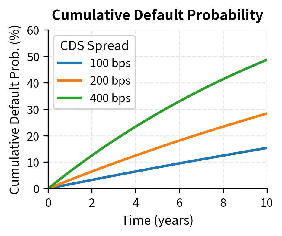
As we discussed in Part II, Chapter 13, CDS spreads provide market-implied default probabilities. This connection is crucial because it allows us to use observable market prices to inform our CVA calculations, rather than relying solely on historical default rates or credit rating agency estimates. For a counterparty with CDS spread and recovery rate , we can extract hazard rates and default probabilities that are consistent with market prices.
The hazard rate (also called the default intensity) represents the instantaneous probability of default conditional on survival to that point. Under a constant hazard rate assumption, the survival probability to time is:
where:
- : probability that the counterparty survives (does not default) until time
- : constant hazard rate (default intensity)
This exponential form arises naturally from the definition of the hazard rate. If the probability of surviving an infinitesimal interval is , then the probability of surviving to time is the product of surviving all the small intervals from 0 to . Taking the continuous limit of this product yields the exponential survival function.
The hazard rate relates to the CDS spread approximately as:
where:
- : hazard rate (default intensity)
- : CDS spread (premium paid for protection)
- : recovery rate (fraction of face value recovered upon default)
This relationship emerges from the economics of a CDS contract, where the premium payments must compensate the protection seller for expected losses. We can derive this approximation by equating the expected cash flows of the two legs of a CDS contract over a short interval :
- Premium Leg: The protection buyer pays spread on the notional amount (set to 1). If survival probability is high (), the payment is approximately .
- Protection Leg: The protection seller pays the loss given default if a default occurs. The probability of default is approximately , so the expected payment is .
Equating the two legs to find the fair spread:
This derivation shows that the CDS spread is approximately equal to the hazard rate multiplied by the loss given default. Intuitively, the protection buyer pays for the expected loss rate, which is the product of how often defaults occur (the hazard rate) and how much is lost when they do (the LGD).
The marginal default probability between and is:
where:
- : probability of default occurring specifically in the interval
- : cumulative survival probability to time
This formula follows directly from the definition of survival probability. The probability of defaulting in a specific interval equals the probability of surviving to the start of the interval minus the probability of surviving to the end. This gives us the probability mass for default in that interval, which is exactly what we need for the discrete CVA formula.
Discounted Expected Exposure
A more precise formulation incorporates discounting, as the loss occurs at the time of default and must be expressed in present value terms:
where:
- : risk-free discount factor from time to
- : expected exposure at time
- : marginal default probability for the interval
- : Loss Given Default
This formulation aggregates the present value of expected losses across all time steps. The logic proceeds as follows: for each time period , we compute the expected loss that would occur if default happens at that time, then discount that loss back to today and weight by the probability of default in that period. Specifically:
- is the expected loss amount if default occurs at
- is the probability of default happening in this specific interval
- discounts that future loss back to today's dollars
Summing these discounted components gives the total upfront price of counterparty risk. This is the amount that should be charged at trade inception to compensate for expected counterparty losses over the life of the contract.
Computing Expected Exposure via Monte Carlo
Calculating expected exposure profiles requires projecting the derivative's value across many future scenarios. This is a forward-looking exercise that demands simulation because, unlike current exposure, future exposure depends on how market conditions might evolve. Monte Carlo simulation, which we covered in Part III, Chapter 10, is the standard approach for this task.
The process involves simulating the underlying risk factors, calculating the derivative's value on each path at each time step, and taking the expected value of positive exposures. This approach is flexible enough to handle complex derivatives and can accommodate multiple risk factors, path dependencies, and optionality. Let's implement this for an interest rate swap.
The Vasicek model, covered in Part III, Chapter 14, provides analytically tractable short-rate dynamics suitable for swap valuation. Each path represents a possible evolution of interest rates over the swap's life. The model's mean-reverting property ensures that simulated rates remain economically plausible over long horizons, neither exploding to infinity nor becoming deeply negative (though negative rates are possible in this model, reflecting the reality of modern interest rate markets).
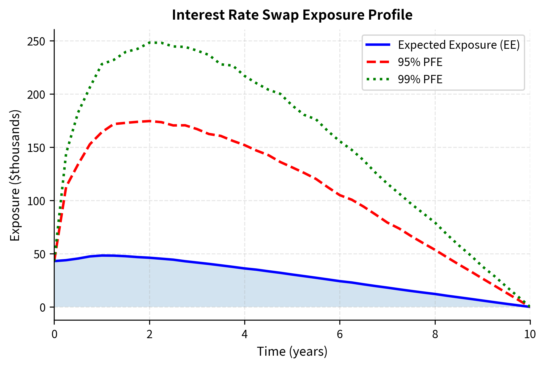
For each simulation path and time step, we compute the swap's mark-to-market value and record the positive part as the exposure. This builds our exposure distribution at each future date. Note that we take the maximum of the swap value and zero, reflecting the fundamental insight that counterparty risk only materializes when the derivative has positive value to us.
The exposure profile displays the characteristic hump shape for interest rate swaps. Early in the swap's life, exposure grows as rates can deviate from their initial values, creating potential gains on the position. Later, exposure declines as fewer payments remain, reducing the maximum possible value regardless of rate movements. The difference between EE and PFE reflects the uncertainty in future exposures; under adverse scenarios (high PFE), the counterparty could owe substantially more than the average. This gap between expected and potential exposure is crucial for credit limit setting, where worst-case scenarios matter more than averages.
CVA Calculation Implementation
With exposure profiles computed, we now calculate CVA by combining expected exposures with default probabilities derived from CDS spreads. This implementation brings together the theoretical framework we developed earlier with practical computation.
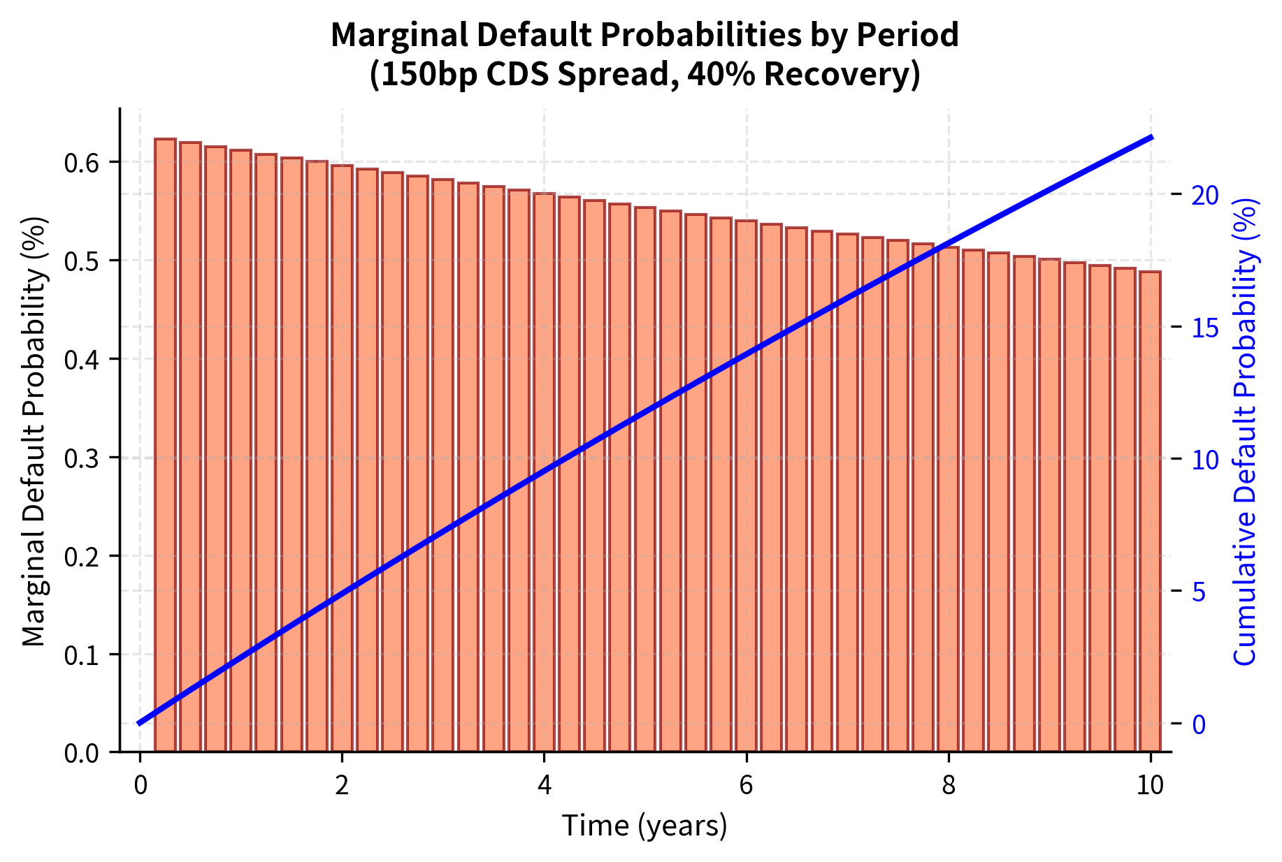
The hazard rate extracted from the CDS spread reflects the market's assessment of the counterparty's creditworthiness. A 150 basis point CDS spread for a counterparty with 40% recovery implies a hazard rate of approximately 2.5% per year. This hazard rate means that, conditional on surviving to any given moment, there is roughly a 2.5% annual probability of defaulting in the next year. The exponential survival function then translates this instantaneous rate into cumulative survival and default probabilities at each future date.
The CVA of approximately 0.25% of notional represents the upfront price of counterparty credit risk for this swap. This amount should be charged to the counterparty or reserved against potential losses. For our portfolio of derivatives, CVA can become a substantial adjustment to firm-wide valuations. A large dealer with hundreds of billions of dollars in derivative notional can have aggregate CVA in the billions, making it a material component of the firm's balance sheet.
Key Parameters
The key parameters for the CVA model are essential to understand because each one significantly influences the final CVA calculation:
- EE: Expected Exposure. The projected future value of the derivative (if positive) averaged across simulation paths. This captures the average amount at risk if default occurs.
- PD: Marginal Probability of Default. The probability of counterparty default occurring within a specific time interval. Higher default probabilities directly increase CVA.
- LGD: Loss Given Default. The portion of the exposure lost upon default, calculated as (1 - Recovery Rate). This represents what fraction of the exposure is actually lost rather than recovered through bankruptcy proceedings.
- D: Discount Factor. The value of a future dollar in today's terms, used to discount expected losses. Losses that might occur far in the future are less costly in present value terms.
- Spread: CDS Spread. The market-observed cost of credit protection, used to infer hazard rates. This is the primary market input for counterparty credit quality.
CVA Sensitivity Analysis
CVA is sensitive to three main drivers: credit quality (CDS spread), exposure profile (driven by market parameters), and recovery assumptions. Understanding these sensitivities is essential for risk management because they tell us which factors matter most for a given position and how CVA might change as market conditions evolve.
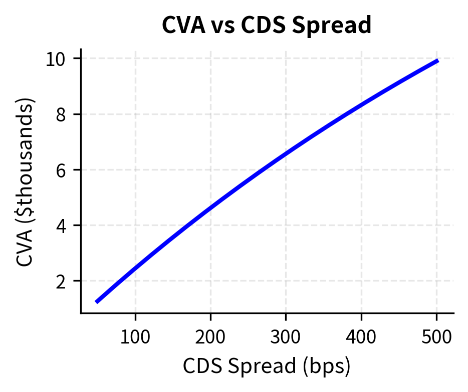
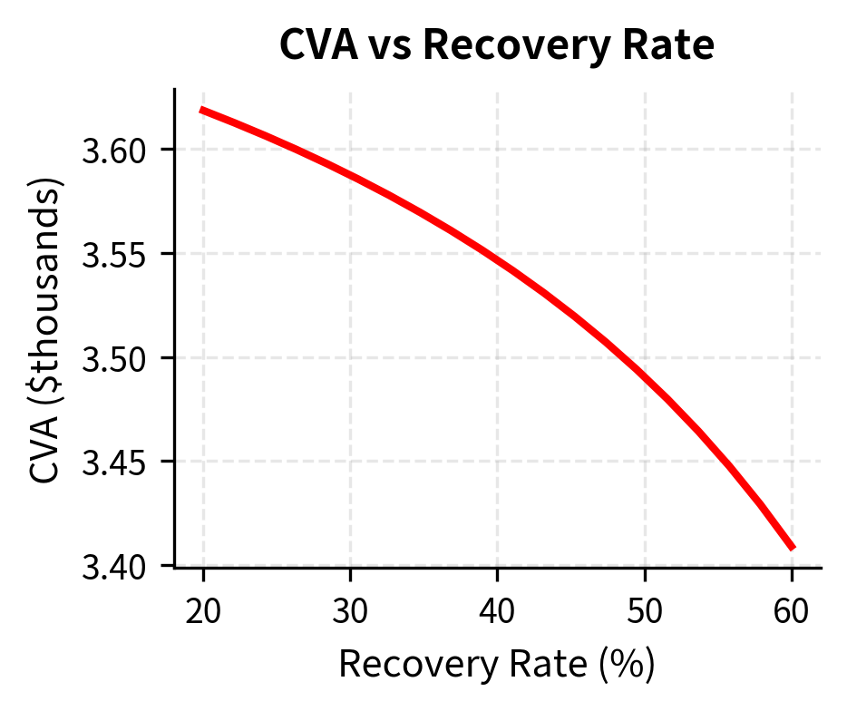
The near-linear relationship between CVA and CDS spread reflects the first-order approximation in the CVA formula. Since default probability is approximately proportional to the hazard rate, and the hazard rate is proportional to the CDS spread, CVA increases roughly linearly with spread. This relationship is extremely useful for hedging, as it suggests that a simple CDS position can offset most of the credit spread risk in CVA.
The recovery rate sensitivity shows a less intuitive pattern: while higher recovery reduces LGD, it also implies lower hazard rates for the same CDS spread, creating offsetting effects. When recovery is high, each default is less costly (lower LGD), but the implied hazard rate from the CDS market is also higher (since the same spread must compensate for smaller expected losses per default, there must be more defaults). These two effects partially cancel, making CVA less sensitive to recovery assumptions than one might initially expect.
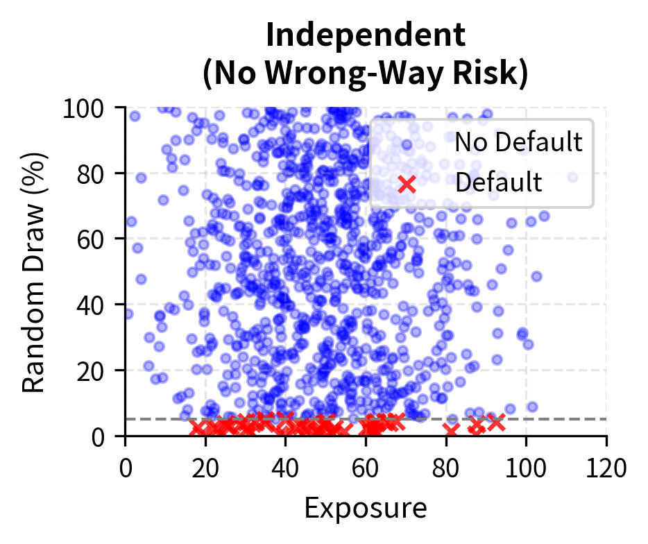
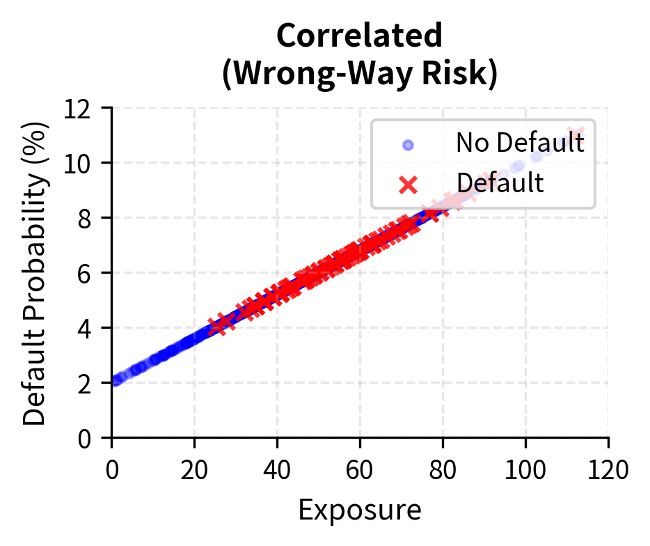
Wrong-Way Risk
A critical complication in CVA modeling is wrong-way risk: the correlation between counterparty default probability and exposure. When these are positively correlated, CVA increases beyond what independent assumptions would suggest. Wrong-way risk can dramatically amplify losses because defaults cluster precisely when exposures are largest.
Wrong-way risk occurs when exposure to a counterparty increases at the same time as their probability of default rises. For example, a commodity producer who sells forward contracts may be more likely to default precisely when commodity prices fall, which is the same scenario where your exposure is highest.
Wrong-way risk comes in two forms, each requiring different modeling approaches:
General wrong-way risk arises from the correlation between macro factors (interest rates, equity markets) and counterparty credit quality. During market stress, many counterparties become more likely to default while derivative exposures increase. For example, in a market crisis, corporate credit spreads widen across the board while equity prices fall. A bank with equity derivatives on multiple corporate counterparties faces both increasing exposure (as equity positions move in their favor) and increasing default probability (as counterparty credit deteriorates).
Specific wrong-way risk occurs when the exposure is directly linked to the counterparty's creditworthiness. The classic example is purchasing put options on a counterparty's stock; the option becomes most valuable exactly when the counterparty is most stressed. Another example is a cross-currency swap with a foreign bank where the bank's creditworthiness is tied to their home country's currency. If the currency weakens significantly, both the swap exposure and the counterparty's default probability increase together.
Modeling wrong-way risk requires joint simulation of market factors and credit events, typically using copula-based approaches to capture the dependence structure. This adds substantial complexity to CVA calculations but is essential for accurate risk measurement. Without wrong-way risk adjustment, CVA can significantly understate the true expected loss, as was demonstrated painfully during the 2008 financial crisis when many assumed-independent risks materialized simultaneously.
Netting and Collateral
Legal documentation significantly affects counterparty exposure through netting agreements and collateral arrangements. These risk mitigation techniques are essential components of modern derivative trading and can reduce CVA by 70% or more in many cases.
Netting
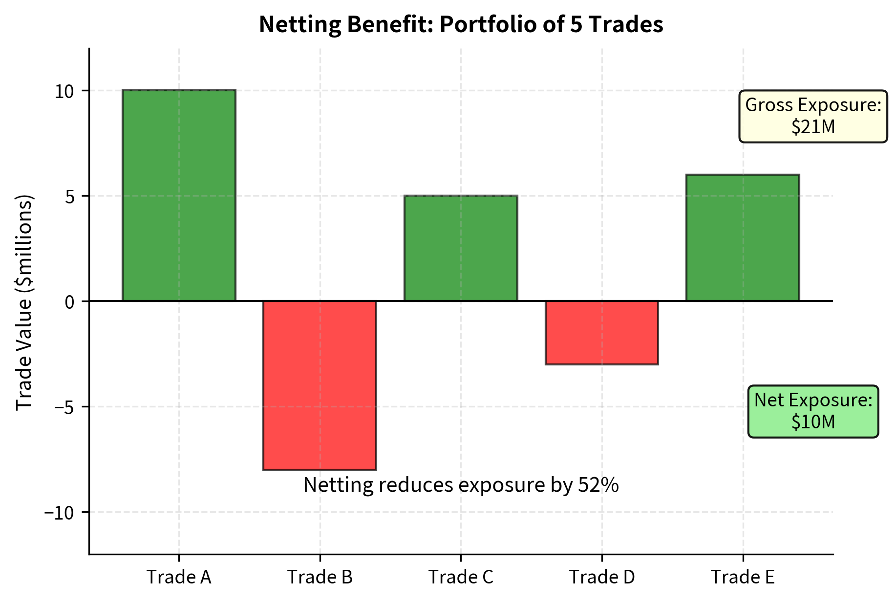
An ISDA Master Agreement typically includes a netting provision that allows offsetting positive and negative positions with the same counterparty. Without netting, you face exposure on all positive-value trades while still owing on negative-value trades. With netting, you can offset these, dramatically reducing net exposure.
To understand the power of netting, consider a simple example. Suppose you have two trades with a counterparty: Trade A has a value of +$10 million (they owe you), and Trade B has a value of -$8 million (you owe them). Without netting, your exposure is $10 million on Trade A, and you still must pay the $8 million on Trade B even if the counterparty defaults. With netting, your net exposure is only \$2 million as the positive and negative values offset.
Mathematically, the comparison is:
compared to:
where:
- : mark-to-market value of the -th trade in the netting set
- : total value of the portfolio allowing for offsets
Netting can dramatically reduce exposure, especially for portfolios with offsetting positions. A dealer with thousands of trades facing a single counterparty might have gross exposure of billions of dollars but net exposure of only millions, representing a reduction of 90% or more.
Collateral and Margining
Credit Support Annexes (CSAs) govern collateral posting. A typical CSA specifies the rules by which counterparties exchange collateral to mitigate credit exposure:
- Threshold: The exposure level above which collateral must be posted
- Minimum Transfer Amount: The smallest collateral transfer required
- Eligible Collateral: Usually cash or high-quality government securities
- Haircuts: Adjustments to collateral value for non-cash securities
Under perfect collateralization with daily margin calls and zero threshold, exposure is limited to one day's potential movement, dramatically reducing CVA. However, during the period between default and closeout (often 10-20 days), exposure can grow, creating residual risk even with collateral. This "margin period of risk" represents the time needed to recognize the default, value the portfolio, liquidate hedges, and close out positions. During this period, the collateral held may become insufficient if market conditions move adversely.
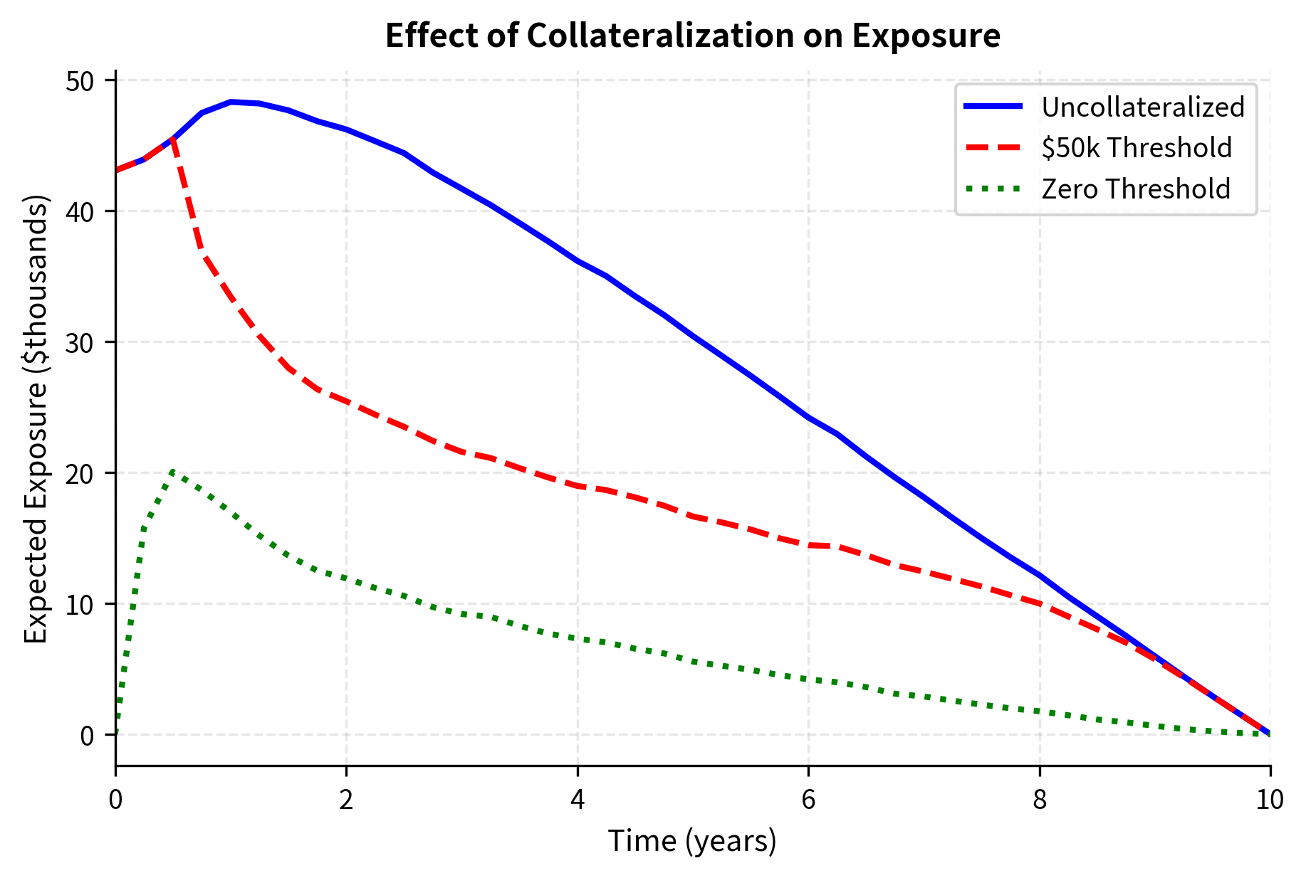
Collateralization substantially reduces exposure, and consequently CVA. This explains why post-crisis regulation pushed for central clearing and mandatory margining of OTC derivatives. The dramatic reduction in exposure under collateralization represents a genuine risk reduction that benefits both counterparties and the financial system as a whole.
The zero-threshold collateralization eliminates most of the CVA, leaving only the risk associated with the margin period of risk. The \$50k threshold introduces a small uncollateralized exposure buffer, resulting in slightly higher CVA, but still achieving a massive reduction compared to the uncollateralized case. These results demonstrate why collateralization has become the norm for interbank derivative trading.
CVA Desk Operations and Hedging
Major banks run dedicated CVA desks that centralize counterparty risk management across the institution. These desks serve several functions and represent one of the most significant organizational innovations in risk management following the 2008 crisis.
Pricing and charging: The CVA desk calculates the CVA for new trades and charges business units accordingly. This ensures that you internalize the cost of counterparty risk when pricing deals. Without this internal charging mechanism, you would have incentive to undercut competitors by ignoring credit risk, ultimately accumulating dangerous exposures.
Hedging: CVA can be hedged using credit default swaps on counterparties. By buying CDS protection, we offset losses from counterparty default. However, hedging is imperfect because:
- CDS may not be liquid for all counterparties
- Wrong-way risk creates correlation that CDS doesn't capture
- Market risk in the exposure profile requires additional hedging
P&L explanation: Changes in CVA flow through the income statement. The CVA desk must explain and manage this volatility, which can be substantial during credit market stress. When counterparty credit spreads widen, CVA increases, creating mark-to-market losses even though no default has occurred.
CVA Hedging Strategy
The sensitivity of CVA to CDS spreads (credit delta) can be hedged by trading CDS. The key insight is that CVA behaves approximately like a portfolio of CDS positions, one for each counterparty, with notional amounts proportional to expected exposure.
where:
- : change in CVA with respect to the credit spread
- : credit spread (hazard rate proxy)
This approximation relies on the linear relationship between CVA and credit spreads: since the default probability is roughly proportional to the spread, CVA scales linearly with . Dividing CVA by the spread gives the sensitivity to spread changes.
For our example swap:
The credit spread sensitivity tells the CVA desk how much CDS protection to purchase. As CDS spreads widen, CVA increases, but the CDS protection pays off, creating an offset. The goal is to match the CS01 of the CVA with the CS01 of the CDS hedge, so that credit spread movements have minimal impact on the combined position.
Regulatory Capital for CVA
Basel III introduced specific capital charges for CVA risk, recognizing that many bank losses during the 2008 crisis came from CVA movements rather than actual defaults. You must hold capital against:
- Credit spread risk: The risk that changes in counterparty credit spreads will move CVA
- Market risk in exposures: The risk that underlying market movements will change exposure profiles
The standardized approach uses a formula based on notional amounts and credit quality, while internal model approaches allow banks to use their own CVA VaR models subject to regulatory approval. The regulatory framework ensures that banks maintain adequate capital buffers against CVA volatility, reducing the risk of capital shortfalls during credit market stress.
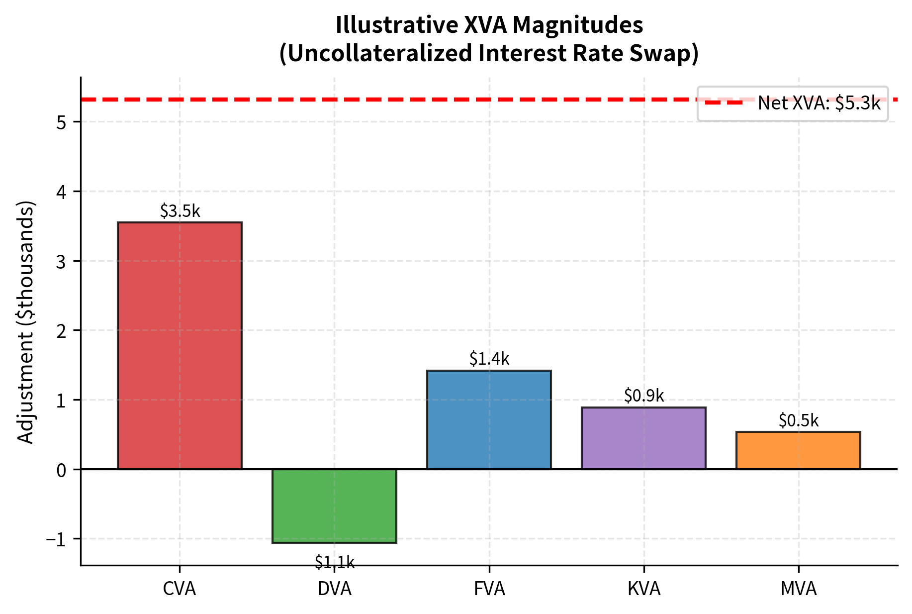
Other Valuation Adjustments (XVA)
CVA was the first of many valuation adjustments that have transformed derivative pricing. The full family of "XVAs" includes several additional adjustments that capture costs and benefits beyond counterparty credit risk.
Debit Valuation Adjustment (DVA)
DVA is the mirror image of CVA; it represents the benefit to you if you default on your obligations. When your own credit spreads widen, your liabilities are worth less in present value terms. While controversial (you benefit from your own deteriorating credit), DVA is required under accounting standards and creates symmetric treatment of bilateral credit risk.
where:
- : your own Loss Given Default
- : Expected Negative Exposure at time (value to counterparty)
- : your own marginal default probability
- : discount factor
The formula mirrors CVA: it aggregates the present value of the debt relief () you would receive if you defaulted, weighted by the probability of your own default in each period. This creates the paradox that a deterioration in your own credit quality increases DVA, improving your P&L, a feature that many find counterintuitive and has sparked ongoing debate in accounting and risk management circles.
Funding Valuation Adjustment (FVA)
FVA reflects the cost of funding uncollateralized derivative positions. If you have a positive exposure to a counterparty without collateral, you must fund that asset at your borrowing rate, which exceeds the risk-free rate. FVA captures this funding cost:
where:
- : funding spread above risk-free rates
- : length of time interval
- : expected exposure requiring funding
- : discount factor
FVA recognizes that uncollateralized derivatives tie up capital that could otherwise be deployed elsewhere. The funding spread represents the premium you pay to borrow unsecured funds, and FVA accumulates this cost over the expected exposure profile of the trade.
Capital Valuation Adjustment (KVA)
KVA accounts for the cost of regulatory capital required to support derivative positions. Regulators require banks to hold capital against potential losses, and this capital has an opportunity cost:
where:
- : required regulatory capital at time
- : cost of capital (hurdle rate)
- : discount factor
- : length of time interval
For each period, the term represents the cost of holding the required regulatory capital. Summing the discounted values of these periodic costs yields the total KVA. This adjustment ensures that trades are priced to deliver adequate returns on the capital they consume.
Margin Valuation Adjustment (MVA)
For cleared trades and bilateral trades under new margin rules, initial margin must be posted. This margin has a funding cost captured by MVA, similar in structure to FVA but applied to margin requirements rather than exposure. Initial margin, unlike variation margin, does not offset exposure dollar for dollar; instead, it provides an additional buffer against potential losses during the closeout period. The funding cost of posting this margin must be incorporated into trade pricing.
The various XVAs interact in complex ways and may involve circular dependencies (e.g., FVA affects pricing, which affects exposure, which affects CVA). Banks have invested heavily in XVA infrastructure, making it one of the most computationally demanding areas of quantitative finance.
Worked Example: Complete CVA Calculation
Let's work through a comprehensive example that brings together all the concepts we have developed. This example demonstrates the complete CVA calculation workflow for a more complex product: a cross-currency swap. Consider a 5-year cross-currency swap where you receive EUR fixed at 2% and pay USD floating (SOFR) on €10 million notional.
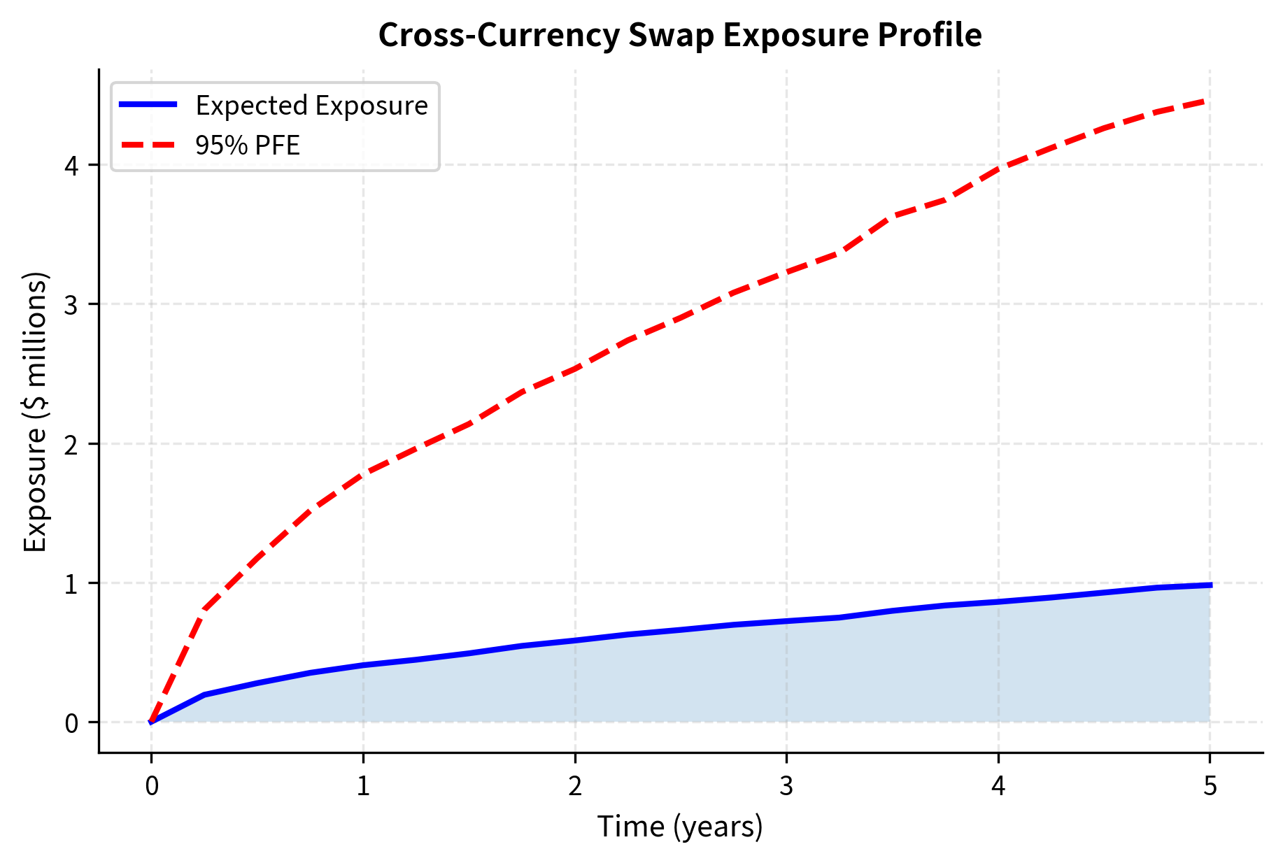
The cross-currency swap shows an exposure profile that increases toward maturity, opposite to the interest rate swap pattern. This reflects the notional exchange at maturity: if EUR/USD moves significantly over five years, the notional exchange creates substantial exposure. The longer the time horizon, the more opportunity there is for the exchange rate to drift from its initial value, and the resulting exposure accumulates until the large final exchange at maturity.
The CVA for this cross-currency swap is substantially higher than for the interest rate swap of similar notional, reflecting both the higher counterparty credit risk (200bp vs 150bp) and the fundamentally different exposure profile with concentration near maturity. This example illustrates why cross-currency swaps receive special attention in counterparty risk management: their exposure profiles are back-loaded, meaning the largest exposures occur precisely when survival probability is lowest.
Key Parameters
The key parameters for the cross-currency swap CVA model are:
- Notional: Principal amount exchanged at maturity. The large final exchange drives exposure.
- Initial FX: The starting exchange rate. Changes in FX rate drive the mark-to-market value.
- : FX volatility. Higher volatility increases potential future exposure and CVA.
- Spread: CDS spread of the counterparty. A higher spread implies higher default probability.
- : USD risk-free rate used for discounting future exposure.
Limitations and Impact
CVA methodology, while now standard across the industry, has important limitations that you must understand. These limitations do not invalidate the approach but rather highlight areas requiring judgment and ongoing research.
Model Risk
CVA calculations depend heavily on models for exposure simulation, default probability estimation, and recovery rate assumptions. The Monte Carlo simulation requires models for underlying risk factors (interest rates, FX, equity prices) that may not capture tail events or regime changes. During the 2008 crisis, many models underestimated correlations during stress, leading to actual losses exceeding CVA provisions. Additionally, the assumption of constant hazard rates extracted from CDS spreads may not hold during credit deterioration, when hazard rates can spike suddenly.
Wrong-Way Risk Challenges
Despite its importance, wrong-way risk remains difficult to model accurately. The correlation between exposure and default probability often manifests only during stress periods that have limited historical data. General wrong-way risk requires macro-economic models that link market stress to credit deterioration, while specific wrong-way risk demands detailed analysis of counterparty-specific exposures. Most industry CVA models incorporate only rough adjustments for wrong-way risk rather than rigorous joint simulation.
Computational Demands
Full CVA calculation for a bank's derivative portfolio requires simulating thousands of counterparties, each with potentially hundreds of trades, across trades, across multiple risk factors and time steps. This creates enormous computational demands, typically addressed through GPU computing, approximation methods, and sensible aggregation. Real-time CVA for trading decisions often uses simplified exposure models rather than full Monte Carlo simulation.
Transformative Impact
Despite these limitations, the development of CVA fundamentally changed derivative markets. Before the 2008 crisis, counterparty risk was often ignored or addressed through ad hoc credit limits. The recognition that CVA represents a real cost has led to several market-wide changes:
- Central clearing: The push for central counterparty clearing of standardized derivatives eliminates bilateral counterparty risk through novation and margin requirements
- Margin reform: New rules require initial and variation margin for uncleared derivatives, substantially reducing exposure
- Pricing transparency: CVA charges are now explicit components of derivative pricing, creating proper incentives for credit risk management
- XVA infrastructure: Banks have invested billions in CVA/XVA systems, creating new specialized roles for quantitative analysts
These changes have made the derivative market more resilient, though at the cost of increased complexity and reduced liquidity for some customized products.
Summary
This chapter covered counterparty credit risk and Credit Valuation Adjustment, essential concepts for anyone working with OTC derivatives.
The key takeaways are:
- Counterparty risk has option-like character: You face losses only when derivatives have positive value at default, creating asymmetric exposure that must be modeled through expected positive exposure
- CVA integrates exposure, default probability, and loss given default: The fundamental formula combines simulated exposure profiles with credit information from CDS markets to produce a fair price for counterparty risk
- Exposure profiles differ by product: Interest rate swaps show hump-shaped profiles, while cross-currency swaps concentrate exposure near maturity; understanding these patterns is crucial for risk management
- Netting and collateral dramatically reduce exposure: Legal documentation through ISDA Master Agreements and CSAs can reduce CVA by 70-90%, explaining the post-crisis push for margining
- CVA desks centralize counterparty risk management: Banks hedge CVA using CDS and manage the P&L volatility from credit spread movements
- The XVA family extends beyond credit: DVA, FVA, KVA, and MVA capture other costs and benefits that affect derivative valuations
CVA calculation remains one of the most computationally intensive areas of quantitative finance, requiring sophisticated simulation techniques and careful modeling of dependencies. As we'll see in the next chapter on liquidity risk, the crisis-era reforms that CVA helped motivate continue to reshape how financial institutions measure and manage risk.
Quiz
Ready to test your understanding? Take this quick quiz to reinforce what you've learned about counterparty credit risk and Credit Valuation Adjustment.

Comments