

Learn Vasicek and CIR short-rate models for interest rate dynamics. Master mean reversion, bond pricing formulas, and derivative valuation techniques.
Choose your expertise level to adjust how many terms are explained. Beginners see more tooltips, experts see fewer to maintain reading flow. Hover over underlined terms for instant definitions.
Short-Rate Interest Rate Models
In Part II, we studied the term structure of interest rates and learned how to extract discount factors and forward rates from observed bond prices. That analysis treated the yield curve as a static object, a snapshot of rates at a single point in time. But interest rates change constantly. The 10-year Treasury yield that was 4.2% yesterday might be 4.3% today and 3.9% next month. To price interest rate derivatives, manage bond portfolio risk, or forecast future rate scenarios, we need models that capture how interest rates evolve through time.
Short-rate models address this need by specifying a stochastic process for the instantaneous interest rate. Building on the Brownian motion and stochastic calculus framework from earlier chapters, these models describe rate dynamics with a combination of deterministic drift and random shocks. The key insight of short-rate models is that once you specify how the instantaneous rate evolves, the entire yield curve at any future time follows from no-arbitrage arguments.
This chapter introduces the two foundational short-rate models: the Vasicek model and the Cox-Ingersoll-Ross (CIR) model. Both incorporate mean reversion, the empirically observed tendency of interest rates to gravitate toward a long-run average level. We'll derive their dynamics, understand their parameters, simulate rate paths, and see how they produce closed-form bond prices. These models laid the groundwork for all subsequent interest rate modeling and remain essential tools for understanding rate dynamics.
The Short Rate and Why We Model It
The short rate is the instantaneous interest rate at time , the rate earned over an infinitesimally small time interval . It represents the continuously compounded rate for borrowing or lending over the next instant.
The short rate is a theoretical construct that serves as the fundamental building block of interest rate modeling. You cannot observe it directly in markets because no instrument has an instantaneous maturity. The closest observable proxies are overnight rates like the federal funds rate or overnight repo rates, but even these apply to discrete time periods rather than true instants. Despite its abstract nature, the short rate serves as a powerful modeling device because it provides a parsimonious way to describe the entire yield curve with a single state variable.
Short rates are fundamental because of their connection to bond prices. If we know how evolves from now until some future time , we can compute the discount factor from the fundamental relationship:
This equation encapsulates the pricing framework. Let's examine each component:
- price at time of a zero-coupon bond paying a face value of 1 at time
- : expectation taken under the risk-neutral measure
- : instantaneous short rate at time
The integral accumulates the short rate over the entire period from to . This accumulated rate, when exponentiated with a negative sign, produces the discount factor. The expectation operator is necessary because is random: we do not know today what the short rate will be at future times . By taking the risk-neutral expectation, we obtain a price consistent with no-arbitrage principles.
This formula, which follows from the risk-neutral valuation framework we developed in Chapter 4 of this Part, tells us that the bond price equals the expected value of the discount factor, where discounting occurs at the random path of short rates. This approach generalizes: once we specify a stochastic process for , we can price any interest rate derivative by computing appropriate expectations of payoffs discounted at this random rate.
A single stochastic differential equation (SDE) for determines the term structure. Different short-rate models make different assumptions about this SDE, leading to different yield curve shapes and dynamics. The choice of SDE reflects your beliefs about how interest rates behave: whether they exhibit mean reversion, how their volatility changes with the rate level, and whether they can become negative.
The Vasicek Model
Model Specification
Oldřich Vašíček's 1977 model established the foundation for modern interest rate modeling. Before this, there was no standard framework for relating interest rate dynamics to bond prices. The Vasicek model assumes the short rate follows an Ornstein-Uhlenbeck process, a continuous-time stochastic process originally developed by physicists to model the velocity of particles subject to friction:
This equation captures key economic behaviors through terms that govern rate evolution:
- speed of mean reversion, controlling how quickly rates return to the long-run mean
- : long-run mean level toward which the process gravitates
- : instantaneous short rate at time
- : volatility of the short rate
- : standard Brownian motion under the risk-neutral measure
The drift term provides mean reversion, the model's defining characteristic. To understand this mechanism, consider what happens in different scenarios. When , the current rate exceeds the long-run mean, making the term negative. Multiplied by the positive constant , this produces a negative drift, pushing rates down toward . Conversely, when , the drift becomes positive, pulling rates up. This self-correcting behavior ensures that rates oscillate around rather than wandering off to arbitrarily high or low values.
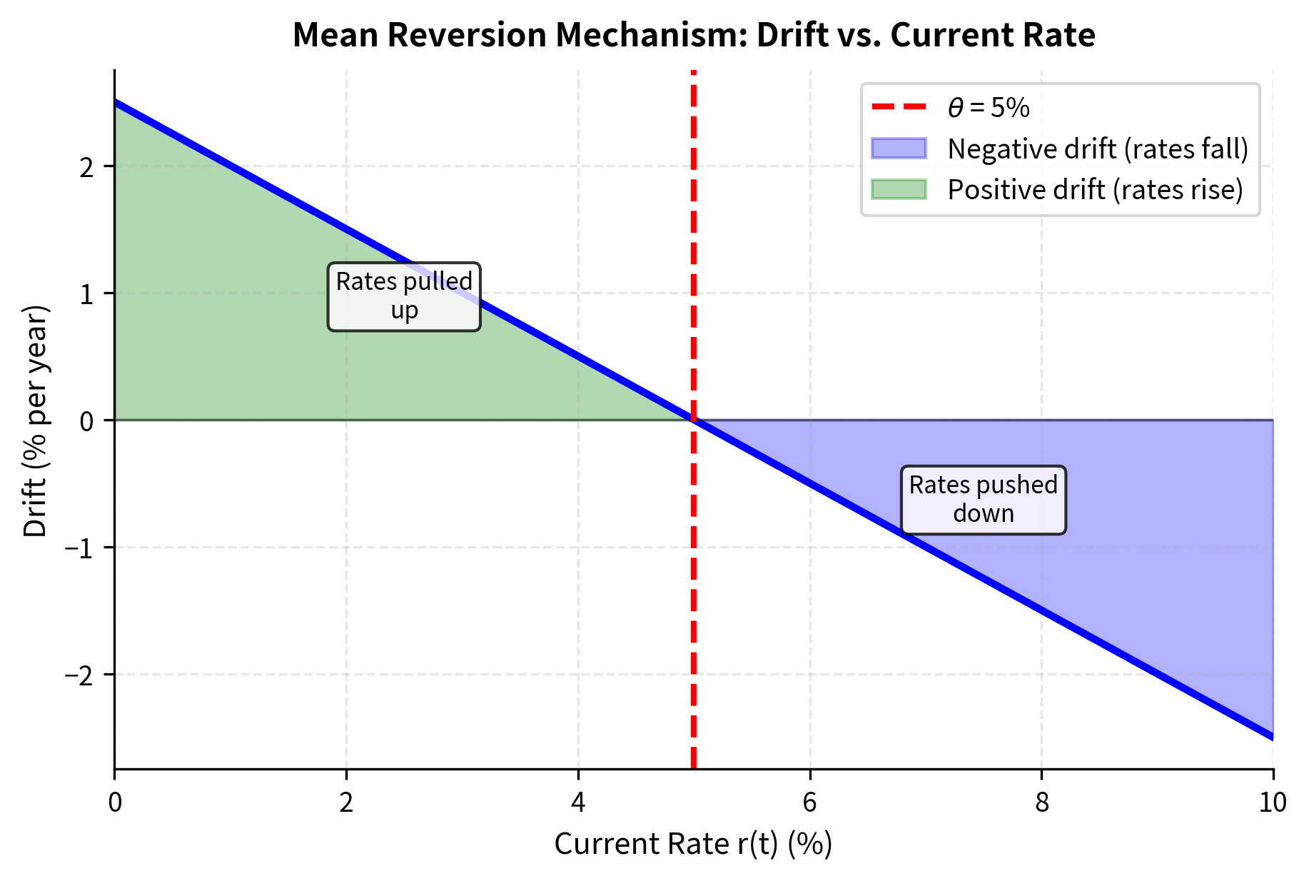
The parameter controls the strength of this gravitational pull. A large means rates snap back quickly after any displacement from , while a small allows rates to deviate from the long-run mean for extended periods. Empirically, interest rates do exhibit mean reversion: extremely high rates tend to fall as central banks loosen policy to stimulate growth, while very low rates eventually rise as economies recover. The Vasicek model captures this economic reality through its mathematical structure.
Solving the SDE
The Vasicek SDE is linear and has an explicit solution, making it useful for practical applications. We solve this using the integrating factor method, a technique familiar from ordinary differential equations. The key insight is to transform the equation into one that can be integrated directly.
Consider the transformation . This choice is motivated by the observation that if we can eliminate the term from the right-hand side, integration becomes straightforward. Applying Itô's Lemma to this transformation, we obtain:
The term from the original drift cancels with the term arising from differentiating the exponential, which is the purpose of this transformation. The resulting expression contains only the deterministic term and the stochastic term , both of which can be integrated directly.
Integrating from to :
The first integral on the right-hand side is a standard calculus integral that evaluates to . The second integral is a stochastic integral against Brownian motion. Multiplying both sides by and rearranging yields the explicit solution:
Each component of this solution has an intuitive interpretation:
- short rate at future time
- : current short rate at time
- : speed of mean reversion
- : long-run mean level
- : volatility of the short rate
- : standard Brownian motion
The first two terms are deterministic, showing how the initial rate decays exponentially toward . The term represents the "memory" of the initial condition, which fades exponentially over time. The term is the complementary contribution from the long-run mean, which grows as the initial condition fades. As becomes large, the first term approaches zero and the second approaches , so the expected future rate converges to the long-run mean regardless of where it started.
The stochastic integral represents accumulated random shocks, with exponential weighting that gives more influence to recent shocks. Shocks that occurred long ago have been "forgotten" due to the mean-reverting drift, while recent shocks still influence the current rate. This weighting function is largest when (equal to 1) and decays for earlier times.
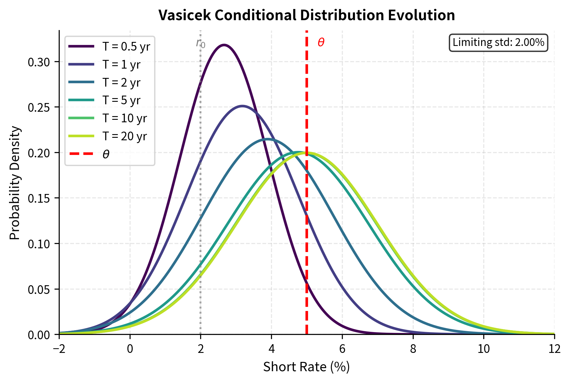
Since the stochastic integral of a deterministic function against Brownian motion is normally distributed (a fundamental property of Itô integrals), conditional on follows a normal distribution:
The conditional mean and variance can be computed explicitly:
These expressions reveal the long-run behavior of the process:
- conditional mean of given
- : conditional variance of given
- : long-run variance of the short rate
- : current short rate
- : mean reversion speed
- : long-run mean
- : volatility
- : time horizon
As the horizon grows large, the conditional mean approaches regardless of the starting point . Similarly, the conditional variance approaches the limiting value , which represents the steady-state variance of the rate process. This limiting variance decreases with stronger mean reversion (larger ) because the process is pulled back toward more frequently, reducing dispersion.
Bond Pricing
The Vasicek model yields analytical formulas for bond prices. The Vasicek model belongs to the class of affine term structure models. This means bond prices have the exponential-affine form
This structure is powerful because the bond price depends on the current short rate in a very specific way: exponentially, with a coefficient that depends only on the time to maturity and model parameters. The components of this expression are:
- price of a zero-coupon bond maturing at
- : deterministic functions of time depending on model parameters
- : current short rate
To derive the specific forms of and , we substitute the assumed form into the fundamental partial differential equation governing bond prices and match coefficients. For the Vasicek model, this procedure yields:
Understanding what these functions represent helps build intuition for bond pricing under mean reversion:
- deterministic functions determining the bond price structure
- : Vasicek model parameters
- : time to maturity
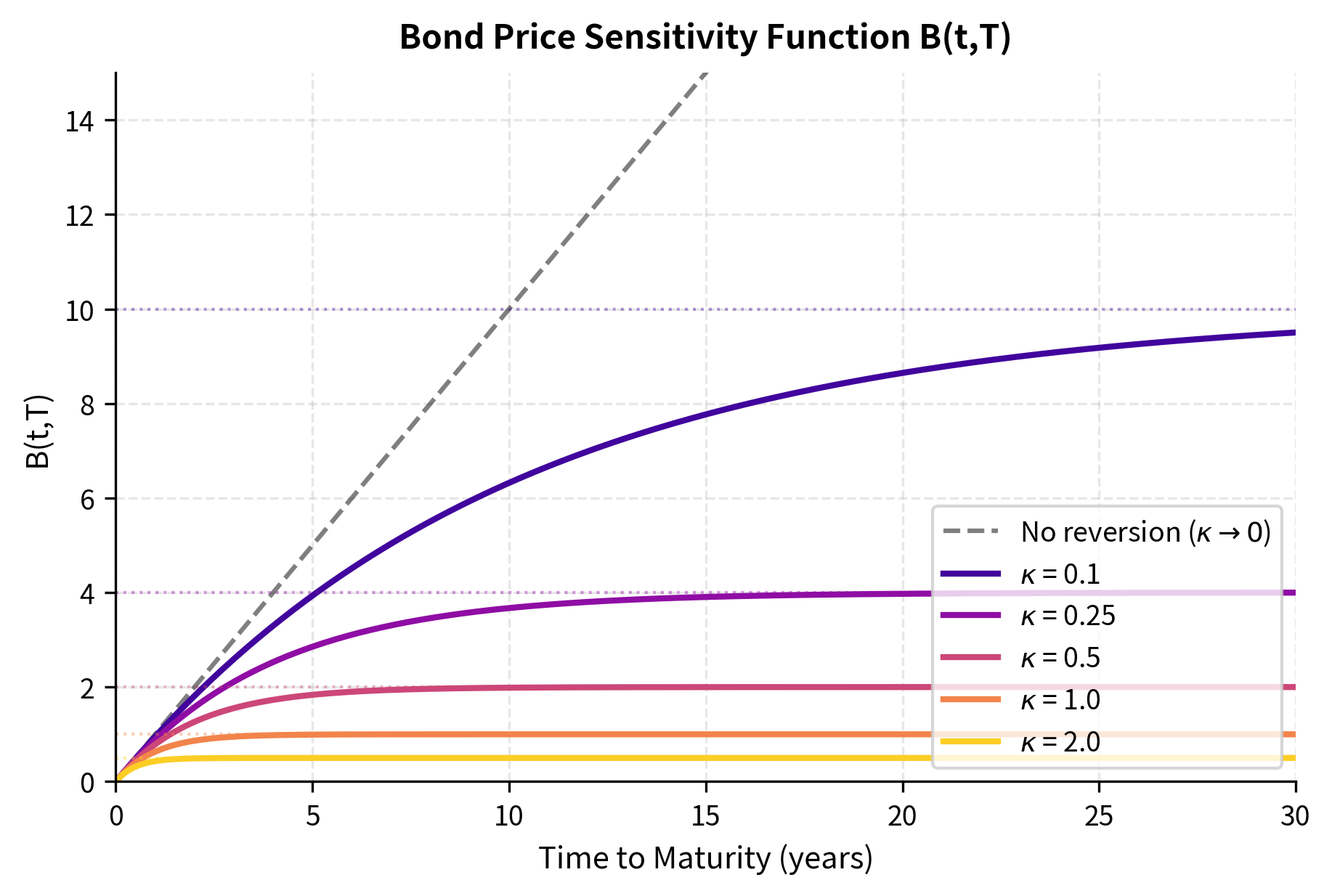
The function measures the sensitivity of the bond price to the short rate, which is closely related to the bond's duration. When is small, approaches , and bond price sensitivity grows linearly with maturity. When is large, the mean reversion prevents long-term rate changes from persisting, so sensitivity saturates at for very long maturities.
The function captures two effects. First, it incorporates the effect of the mean-reverting drift toward . Second, it includes a convexity adjustment arising from volatility. This adjustment reflects the fact that bondholders benefit from interest rate volatility due to the convex relationship between rates and prices: when rates fall, prices rise more than they fall when rates rise by the same amount.
These closed-form expressions make the Vasicek model computationally tractable. Given parameters and the current short rate , you can instantly compute the price of any zero-coupon bond and therefore construct the entire yield curve. This stands in contrast to models without analytical solutions, which require time-consuming numerical methods.
The continuously compounded yield for maturity follows directly from the bond price:
This expression shows that the yield is an affine (linear plus constant) function of the short rate:
- continuously compounded yield for maturity
- : zero-coupon bond price
- : Vasicek model functions defined above
- : time to maturity
- : current short rate
The affine structure extends to yields, which is why this class of models is called "affine term structure models." The linearity of yields in the short rate has important implications: parallel shifts in the short rate produce parallel shifts in the yield curve, scaled by the maturity-dependent factor .
The Negative Rate Problem
A critical feature of the Vasicek model is that is normally distributed, which means it can take negative values with positive probability. For decades, this was considered a significant drawback of the model. How could interest rates be negative? The reasoning went that if deposit rates were negative, banks would pay you to borrow money, which seemed economically absurd. Rational agents would simply hold cash rather than accept negative returns.
Then came the post-2008 financial crisis era. Central banks in Europe, Japan, and Switzerland pushed policy rates below zero in an effort to stimulate lending and economic activity. Suddenly, negative rates were not just theoretically possible but empirically observed. Banks charged depositors for holding their money, and some government bonds traded at negative yields.
The Vasicek model's ability to generate negative rates transformed from a bug to a feature for modeling modern interest rate environments. While the model was not designed with negative rates in mind, its mathematical structure accommodates this reality naturally. This historical reversal illustrates an important principle: model properties that seem problematic under one economic regime may become valuable under different circumstances.
The Cox-Ingersoll-Ross Model
Model Specification
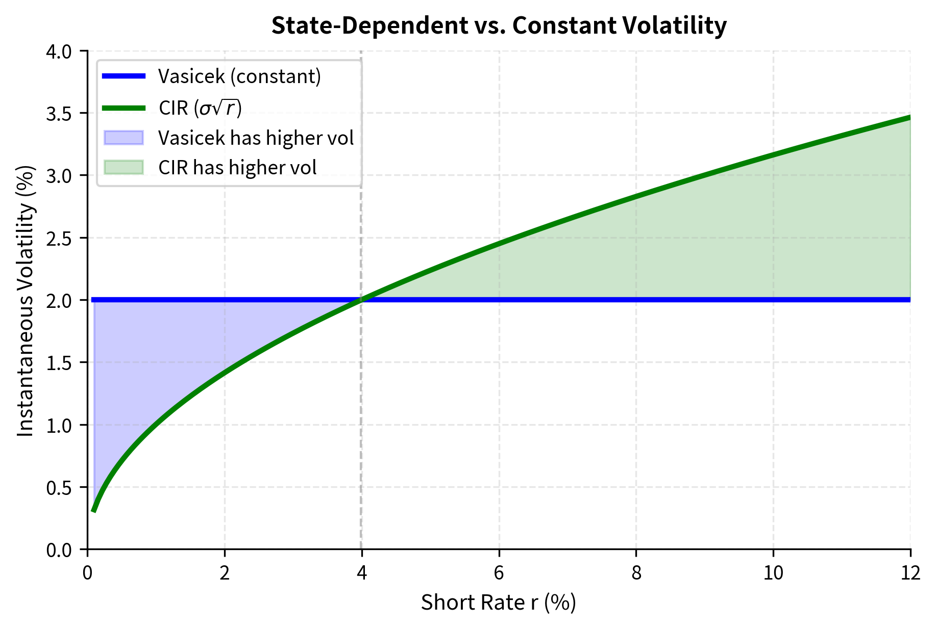
John Cox, Jonathan Ingersoll, and Stephen Ross developed their model in 1985 as part of a general equilibrium framework for asset pricing. Unlike Vasicek, who specified the rate dynamics directly, Cox, Ingersoll, and Ross derived their model from underlying assumptions about technology, preferences, and market equilibrium. The CIR model modifies the Vasicek specification by making volatility proportional to the square root of the rate:
The drift term is identical to Vasicek, preserving the mean-reverting structure. The key innovation lies in the diffusion term:
- mean reversion speed and long-run mean
- : volatility coefficient
- : state-dependent volatility scaling factor
- : Brownian increment
The parameters , , and have the same interpretations as in Vasicek: mean-reversion speed, long-run mean, and volatility coefficient respectively. The crucial difference is the term multiplying the Brownian shock.
This square-root diffusion has profound implications for the behavior of the process. When is close to zero, the volatility term becomes small, reducing the chance of large negative shocks that could push rates below zero. The process essentially "quiets down" as it approaches zero. When is larger, volatility increases proportionally, matching the empirical observation that rate volatility tends to be higher during high-rate environments. Historical data shows that volatility depends on the rate level.
The economic intuition behind the square-root specification connects to the general equilibrium derivation. In the Cox-Ingersoll-Ross framework, the interest rate is linked to the marginal product of capital in the economy. When rates are low, the economy is in a depressed state with limited investment opportunities, and uncertainty about future rates is also low. When rates are high, the economy is more active, and there is greater uncertainty about the path of future rates.
The Feller Condition
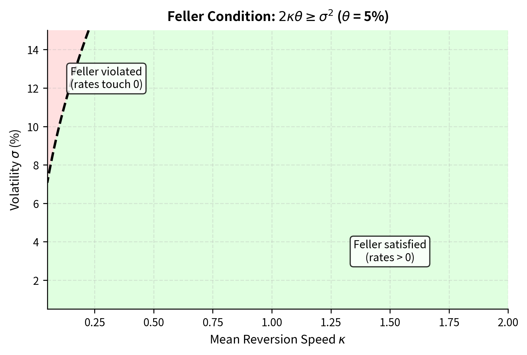
The CIR model keeps rates non-negative under certain parameter restrictions. The Feller condition states:
This inequality places a constraint on the relationship between model parameters:
- mean reversion speed
- : long-run mean
- : volatility parameter
When this condition holds, the rate will never hit zero. If it is violated, rates can touch zero but will immediately bounce back; they cannot become negative. This distinction matters for certain theoretical analyses but has limited practical impact, as rates near zero behave similarly in both cases.
The Feller condition ensures the short rate in the CIR model remains strictly positive. It requires that the mean-reversion drift toward is strong enough relative to volatility to prevent rates from reaching zero.
The intuition behind the Feller condition is straightforward when viewed as a balance of forces. The condition compares two quantities: the deterministic pull toward (captured by , which represents how fast the drift pushes rates up when they are near zero) and the random shocks (captured by , which measures the magnitude of random fluctuations). If volatility is too high relative to the mean-reversion strength, the random shocks can overwhelm the upward drift near zero, potentially pushing the process to zero despite the drift trying to keep it positive.
The factor of 2 in the condition arises from the mathematical properties of the square-root process. When is small, the drift is approximately (since is negligible), while the variance of shocks is approximately . For the drift to dominate near zero, we need to exceed the standard deviation of shocks, which leads to the Feller condition after careful analysis.
Distribution of Future Rates
Unlike the Vasicek model, the CIR process does not yield normally distributed rates. The square-root diffusion produces a fundamentally different distribution. Specifically, conditional on follows a non-central chi-squared distribution, a probability distribution that arises naturally in statistics when summing squares of normal random variables:
The non-central chi-squared distribution is characterized by two parameters:
- non-central chi-squared random variable
- : degrees of freedom
- : non-centrality parameter
For the CIR model, these parameters are:
The degrees of freedom depends only on the model parameters and is constant over time. Notice that when the Feller condition holds exactly (with equality), . The non-centrality parameter depends on the current rate and decreases as the horizon increases, reflecting the fading influence of the initial condition. The remaining notation:
- CIR model parameters
- : current short rate
- : time horizon
The conditional mean and variance can be computed from the properties of the non-central chi-squared distribution:
These formulas reveal an important relationship between the Vasicek and CIR models:
- conditional expected value of the rate
- : conditional variance of the rate
- : current short rate
Notice that the conditional mean formula is identical to the Vasicek model; both processes have the same expected path. The mean reversion operates identically in both cases, pulling rates toward at speed . The difference lies in the variance structure and the shape of the distribution. The CIR variance has two terms: one proportional to (reflecting the state-dependent volatility) and one proportional to (the contribution from shocks accumulated as the process approaches its steady state).
The non-central chi-squared distribution is positively skewed, unlike the symmetric normal distribution of Vasicek. This skewness becomes more pronounced when rates are low, as the distribution is bounded below by zero but can extend to high values. When rates are high, the distribution becomes more symmetric and approaches normality, consistent with the central limit theorem as the non-centrality parameter grows.
Bond Pricing
The CIR model is also affine, with bond prices taking the form . The derivation follows the same approach as Vasicek: substitute the assumed form into the bond pricing PDE and solve for the coefficients. The resulting functions are:
The auxiliary parameter that appears in these formulas combines the model parameters in a specific way:
- deterministic functions for the CIR bond price
- : auxiliary parameter
- : CIR model parameters
The parameter can be interpreted as an "adjusted" mean-reversion speed that accounts for the risk premium embedded in bond prices. It is always larger than , reflecting that bonds are priced as if rates reverted faster than they actually do under the physical measure.
While more complex than the Vasicek formulas, these expressions remain analytically tractable and enable rapid bond pricing without numerical integration. As in the Vasicek model, measures the bond's sensitivity to the short rate (duration), while captures the effects of mean reversion and the convexity adjustment. The CIR formulas reduce to the Vasicek formulas in the limit as the square-root term becomes approximately constant (which occurs when rate levels are high relative to their volatility).
Comparing Vasicek and CIR
The table below summarizes the key differences between the two models:
| Feature | Vasicek | CIR |
|---|---|---|
| Diffusion | Constant () | State-dependent () |
| Rate distribution | Normal | Non-central chi-squared |
| Negative rates | Possible | Not possible (with Feller condition) |
| Volatility behavior | Constant | Higher when rates are high |
| Analytical tractability | Simpler formulas | More complex but still closed-form |
Both models share the same mean-reversion structure, producing similar expected rate paths. The primary differences concern:
-
Distributional assumptions Vasicek assumes normal shocks regardless of rate level; CIR assumes volatility scales with rate level.
-
Positivity: CIR guarantees non-negative rates when the Feller condition holds; Vasicek does not.
-
Empirical fit: CIR's state-dependent volatility often better matches observed rate dynamics, where volatility tends to be higher during high-rate periods.
Simulation of Short-Rate Paths
Let's implement both models and visualize their behavior. We'll start by simulating multiple paths to understand how mean reversion shapes rate dynamics.
Vasicek Simulation
The Vasicek model admits two approaches to simulation. The simpler approach uses Euler-Maruyama discretization which approximates the continuous-time SDE with discrete time steps. The discretization follows the general pattern of replacing with , with , and with where is standard normal:
The components of this discrete recursion are:
- rate at the next time step
- : time step size
- : standard normal random variable,
- : current rate
- : Vasicek parameters
Since the Vasicek model has an exact solution, we can also simulate using the exact transition density. This approach is superior because it produces samples from exactly the correct distribution regardless of time step size, eliminating discretization error. The implementation below uses this exact simulation method.
CIR Simulation
For the CIR model, exact simulation is more complex due to the non-central chi-squared transition distribution. While exact methods exist (involving transformations to chi-squared random variables), practitioners often use the Euler-Maruyama scheme with a reflection or truncation to handle potential negative values:
Each term in this discretization corresponds to its continuous-time counterpart:
- standard normal random variable
- : diffusion term dependent on current rate level
- : rate at next step
- : current rate
- : CIR parameters
- : time step size
The challenge with this discretization is that the right-hand side can become negative even though the continuous-time process stays positive. This occurs because the discrete approximation does not perfectly capture the behavior of the square-root diffusion near zero. We apply a full truncation scheme where we take before computing the square root, and again after adding the shock. This is one of several approaches in the literature; alternatives include reflection schemes and implicit methods.
The Feller condition is satisfied with these parameters, so the CIR model should keep rates strictly positive.
Visualizing Path Behavior
Let's plot sample paths from both models to see mean reversion in action.
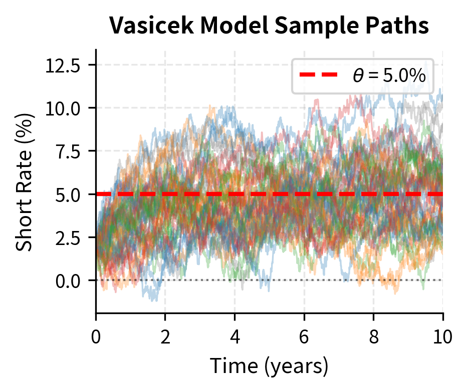
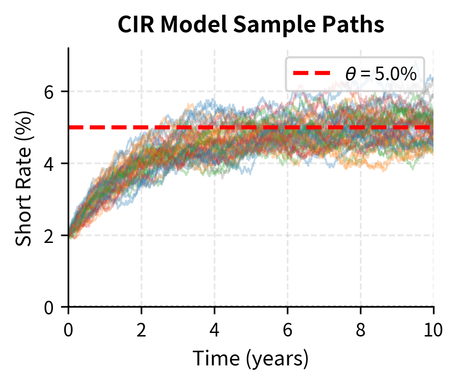
The models show clear mean reversion. Paths starting at 2% tend to drift upward toward the 5% long-run mean. The key visual difference is that some Vasicek paths dip below zero, while CIR paths remain positive throughout.
Distribution Analysis
Let's examine the distribution of rates at the 10-year horizon.
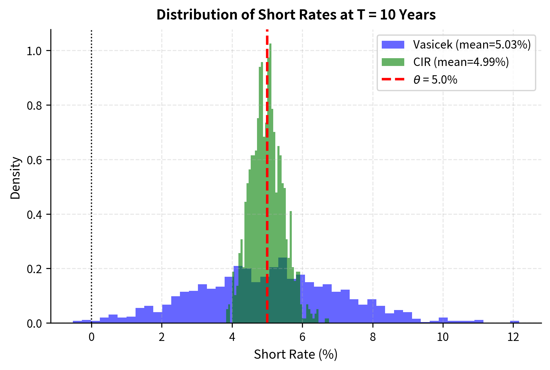
Both models converge toward the theoretical mean of approximately 5%, as expected from the mean-reversion dynamics. The Vasicek distribution is symmetric and normal, while the CIR distribution shows slight right-skewness and is bounded below by zero.
Bond Pricing with Short-Rate Models
Vasicek and CIR models provide closed-form bond pricing formulas. Let's implement these and construct yield curves.
Yield Curve Construction
Let's generate yield curves for different initial short rates.
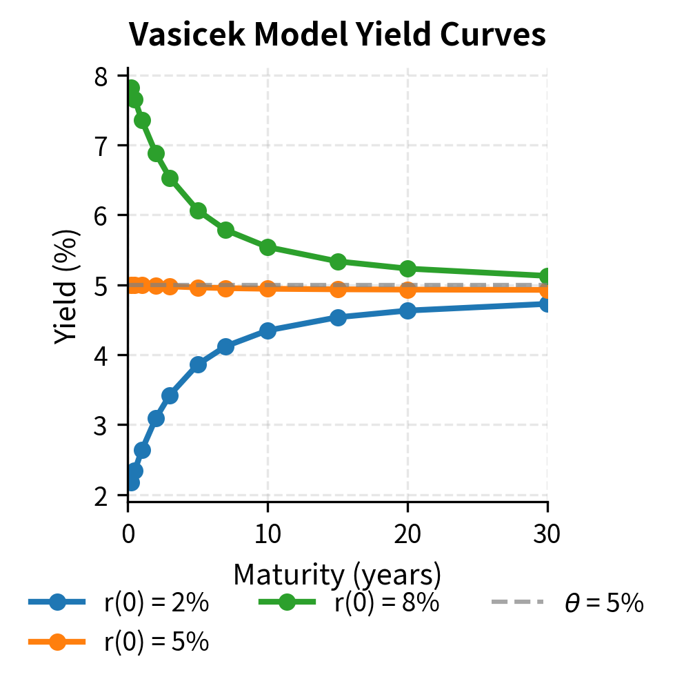
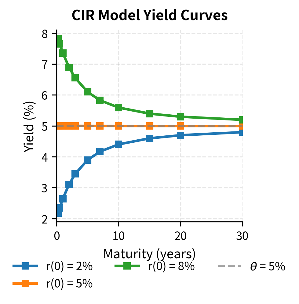
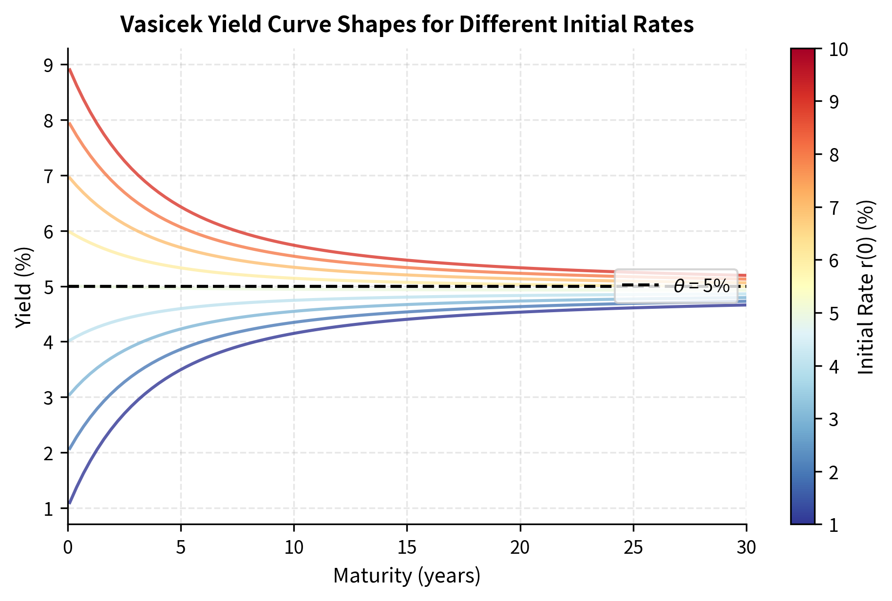
The yield curves demonstrate several important features of mean-reverting short-rate models:
-
Convergence: All curves converge toward a common long-term yield regardless of the initial rate. This reflects the mean-reversion property, where expected rates eventually gravitate toward .
-
Curve shape flexibility: When , the yield curve is upward-sloping (normal). When , the curve is downward-sloping (inverted). When , the curve is relatively flat but shows a slight convexity effect.
-
Risk premium implicit in long yields: Long-term yields don't equal exactly due to the interaction between mean reversion and interest rate volatility, which creates a convexity adjustment in bond prices.
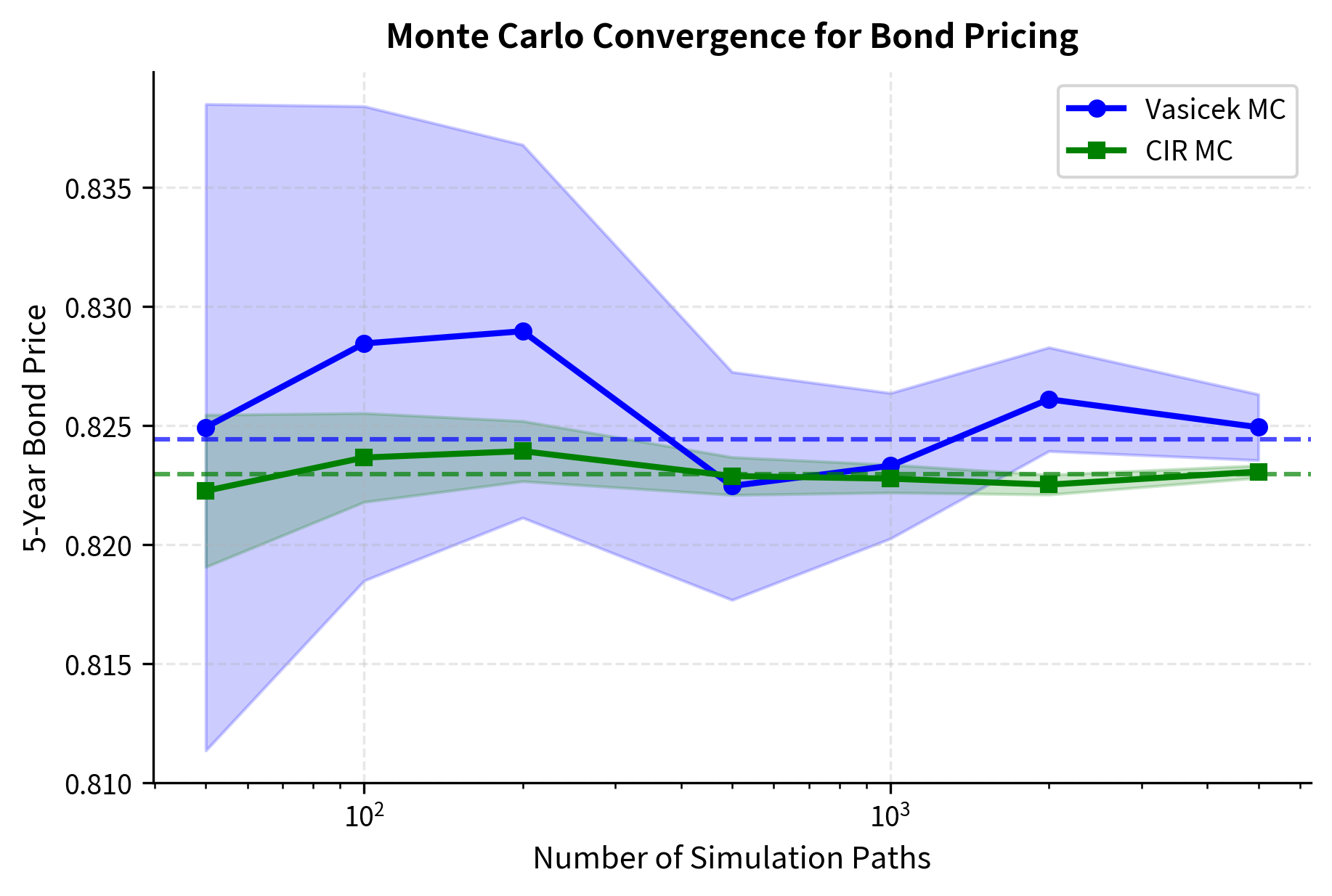
Monte Carlo Bond Pricing
We can also price bonds using Monte Carlo simulation by averaging the discount factor across paths. This approach is more general than the closed-form solutions and extends to models without analytical formulas.
The Monte Carlo estimator for the zero-coupon bond price is:
This formula averages the realized discount factors across all simulated paths:
- number of simulation paths
- : number of time steps
- : short rate on path at step
- : time step size
The inner sum approximates the integral for path using a Riemann sum. The exponential of the negative of this integral gives the discount factor for that path. Averaging across all paths produces an unbiased estimator of the bond price, with standard error decreasing as .
This approach generalizes to complex interest rate derivatives. For any derivative with payoff depending on rates at multiple times, we can estimate the price by simulating paths, computing the payoff on each path, discounting at the realized short-rate integral, and averaging.
The Monte Carlo estimates closely match the analytical formulas, validating our simulation implementation. The small differences arise from simulation error, which decreases with more paths or finer time steps.
Pricing Interest Rate Derivatives
Short-rate models enable pricing of various interest rate derivatives. Let's implement a simple example: pricing a zero-coupon bond option.
European Bond Options
Under the Vasicek model, European options on zero-coupon bonds have closed-form solutions. These formulas resemble the famous Black-Scholes formula for stock options, but with modifications appropriate for the interest rate setting. A call option on a -maturity bond, expiring at time , gives the holder the right to purchase the bond at the strike price . The value of this option is:
Each term in this pricing formula has a clear interpretation:
- value of the European call option
- : price of zero-coupon bond maturing at
- : strike price
- : cumulative standard normal distribution function
- : standardized limits for the integration
- : volatility of the forward bond price
The first term represents the expected present value of receiving the bond, weighted by the probability (under an appropriate measure) that the option will be exercised. The second term represents the expected present value of paying the strike price, again weighted by the exercise probability under the risk-neutral measure.
The parameters and measure how far the current forward price is from the strike, scaled by volatility:
The numerator of the first term in compares the forward price of the underlying bond (which equals in a no-arbitrage setting) to the strike price :
- standardized integration limits
- : zero-coupon bond prices
- : strike price
- : volatility of the forward bond price
The volatility term measures how much uncertainty there is about the bond price at the option's expiration. In the Vasicek model, this volatility can be computed analytically:
This expression combines several factors that contribute to bond price uncertainty:
- volatility of the short rate
- : Vasicek bond coefficient
- : option expiration time
- : bond maturity time
- : mean reversion speed
The factor is the underlying volatility of the short rate. The factor translates short-rate volatility into bond price volatility for a bond maturing at , as of the option expiration at . The square-root term accounts for the accumulation of uncertainty from now until the option expiration, adjusted for mean reversion. Stronger mean reversion (larger ) reduces uncertainty because the rate is pulled back toward more quickly.
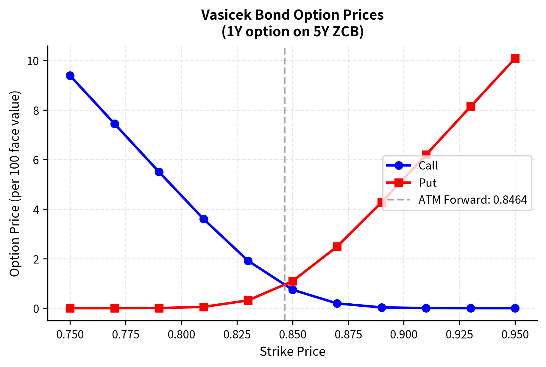
The option prices follow familiar patterns: calls decrease as strike increases, puts increase as strike increases. The intersection near the ATM forward strike reflects put-call parity for bond options.
Key Parameters
The key parameters for the Vasicek and CIR models govern all aspects of rate dynamics and derivative pricing:
-
Instantaneous short rate. The fundamental state variable driving the term structure. All bond prices and yields are functions of this single variable, which is why these are called "one-factor" models.
-
: Speed of mean reversion. Controls how quickly the rate returns to the long-run mean . Larger values of produce tighter distributions around and faster convergence of yield curves to their long-term levels.
-
: Long-run mean level. The equilibrium level toward which interest rates gravitate over time. This parameter reflects structural factors in the economy such as potential growth rates and inflation expectations.
-
: Volatility of the short rate. Determines the magnitude of random shocks affecting the rate path. In Vasicek, this is an absolute volatility; in CIR, it is scaled by the square root of the rate level.
-
: Time to maturity. Used in bond and option pricing formulas. The effect of maturity on prices depends on the interplay between mean reversion and volatility.
-
: Strike price. The exercise price for bond options. Together with the forward price of the underlying, the strike determines the moneyness of the option.
Parameter Impact Analysis
Exploring how parameters affect rate dynamics and bond prices helps build intuition for calibration.
Effect of Mean Reversion Speed
The parameter controls how quickly rates revert to the long-run mean. Higher means faster reversion and lower variance in the long run.

With low , rates wander more freely and take longer to approach . With high , rates snap back quickly after any shock, resulting in a tighter distribution around the long-run mean.
Effect of Volatility
The volatility parameter scales the random component. Higher volatility produces wider distributions and more variable rate paths.
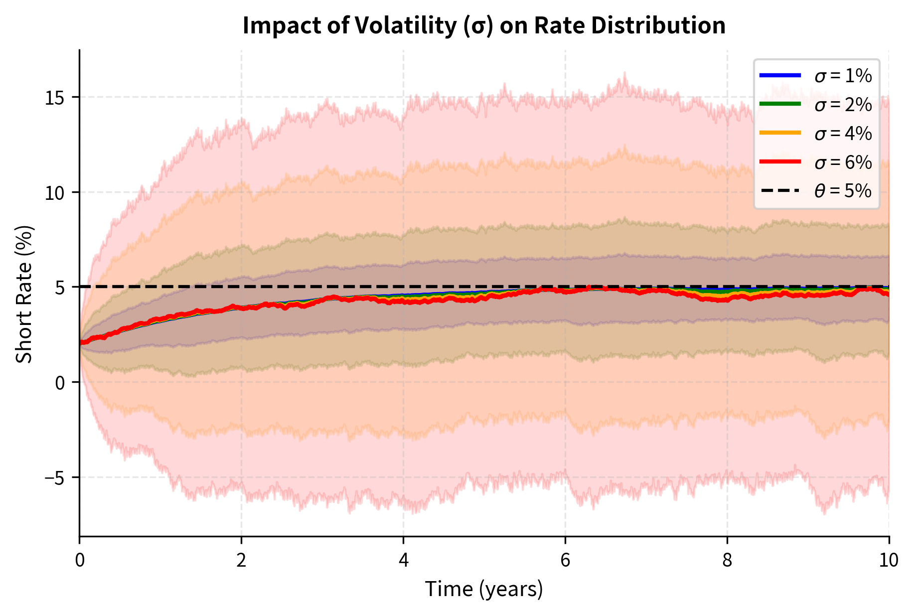
The mean paths are nearly identical across volatility levels since doesn't affect the expected rate path, only its variance. Higher volatility dramatically widens the confidence bands, increasing the probability of extreme rate scenarios.
Yield Curve Shapes
The interplay between parameters determines what yield curve shapes the model can produce. Let's explore how the current rate relative to the long-run mean affects the curve.
The Vasicek model (and CIR) can produce a range of yield curve shapes, but with important limitations. Both models belong to the class of single-factor models, meaning all yields are driven by a single source of randomness. This implies that yields at different maturities are perfectly correlated, which is not observed in practice where short and long rates sometimes move in opposite directions.
Limitations and Impact
What These Models Enabled
The Vasicek and CIR models represented a major advance in fixed-income modeling when introduced in the 1970s and 1980s. They provided the first rigorous, arbitrage-free frameworks for understanding how interest rates evolve and how this evolution affects derivative prices. Their key contributions include:
The concept of mean reversion in rates became standard. Before these models, practitioners often assumed rates followed random walks without drift, which implied rates could wander arbitrarily far from any long-run level. The mean-reverting specification captured the economic intuition that extremely high or low rates are unsustainable and markets tend to push rates back toward equilibrium levels. This insight continues to inform all modern interest rate modeling.
Closed-form bond pricing formulas enabled practical applications. The affine structure of both models means that bond prices, forward rates, and many derivative prices can be computed analytically without resorting to simulation or numerical methods. This computational efficiency was crucial in the pre-computer-intensive era and remains valuable today for calibration and real-time pricing.
The models also established the template for equilibrium-based interest rate modeling. Both Vasicek and CIR derived their dynamics from underlying assumptions about the economy and investor behavior, grounding the mathematical specification in economic theory rather than pure statistical convenience.
Key Limitations
Despite their foundational importance, these single-factor short-rate models have significant limitations that led to the development of more sophisticated approaches.
The most fundamental limitation is the single-factor structure. With only one source of randomness driving all rates, yields across the entire term structure are perfectly correlated. In reality, central bank actions might push short rates down while inflation concerns push long rates up, creating correlation structures that single-factor models cannot capture. Multi-factor extensions address this but sacrifice some analytical tractability.
Another critical issue is the inability to match the current yield curve exactly. Both models produce yield curves as functions of their parameters, but for any fixed parameter set, the model-implied curve will generally differ from the observed market curve. This means you cannot use these models to price derivatives consistently with observed bond prices unless you either accept some pricing errors or use time-varying parameters.
The Vasicek model's potential for negative rates was historically seen as a flaw, though the post-2008 era of negative policy rates made this feature more acceptable for certain applications. However, the CIR model's requirement that the Feller condition hold can make calibration to historical data challenging, as estimated parameters may violate this constraint.
Both models also assume constant parameters over time. Real interest rate dynamics exhibit regime changes: the high-volatility period of the early 1980s differs dramatically from the low-rate, low-volatility environment of the 2010s. Constant-parameter models cannot capture these shifts without re-estimation.
The Path Forward
These limitations motivated the development of more advanced interest rate models. The Heath-Jarrow-Morton (HJM) framework and LIBOR Market Model (LMM), which we'll explore in the next chapter, address the calibration issue by modeling the entire forward curve rather than just the short rate. Multi-factor models incorporate additional sources of randomness to capture realistic correlation structures. The calibration techniques covered in Chapter 21 provide methods for fitting model parameters to market data while respecting no-arbitrage constraints.
Despite their limitations, Vasicek and CIR remain important for building intuition about rate dynamics, for educational purposes, and as building blocks within more complex models. Understanding these foundational models is essential before tackling the more advanced frameworks used in modern practice.
Summary
This chapter introduced short-rate models, which describe the evolution of the instantaneous interest rate as a stochastic process with mean reversion. The key concepts covered include:
The short rate is the instantaneous interest rate driving all bond prices through the relationship . Specifying a stochastic process for determines the entire term structure dynamics.
The Vasicek model was the first mean-reverting short-rate model. It produces normally distributed rates, allowing for negative values, and has simple closed-form bond pricing formulas with exponential-affine structure.
The CIR model modifies Vasicek by making volatility proportional to . This keeps rates non-negative when the Feller condition holds, producing chi-squared distributed rates with state-dependent volatility.
Mean reversion is the central feature of both models. The parameter controls how fast rates return to the long-run mean after a shock. Higher means faster reversion and lower long-run variance.
Yield curves under these models converge to a common long-term rate regardless of the initial short rate. The shape depends on whether is above or below , producing inverted, flat, or normal curves.
Limitations include the single-factor structure (perfect correlation across maturities), inability to match observed yield curves exactly, and constant parameters that cannot capture regime changes.
These models laid the foundation for all modern interest rate modeling. The next chapter examines advanced frameworks like HJM and the LIBOR Market Model that address some limitations while preserving the arbitrage-free pricing foundation established here.
Quiz
Ready to test your understanding? Take this quick quiz to reinforce what you've learned about short-rate interest rate models.

Comments