

Master the Heath-Jarrow-Morton framework and LIBOR Market Model for pricing caps, floors, and swaptions. Implement forward rate dynamics in Python.
Choose your expertise level to adjust how many terms are explained. Beginners see more tooltips, experts see fewer to maintain reading flow. Hover over underlined terms for instant definitions.
Advanced Interest Rate Models (HJM and LMM)
In the previous chapter, we explored short-rate models like Vasicek, CIR, and Hull-White, which describe the evolution of the instantaneous short rate . While these models provide elegant closed-form solutions for bond prices and some derivatives, they face a fundamental limitation: starting from a single factor (the short rate), they derive the entire term structure of interest rates. This approach often struggles to match the rich dynamics observed in real yield curves and can produce unrealistic implied volatility structures for interest rate derivatives. This gap between simple models and market reality led to frameworks that better capture interest rate behavior.
The Heath-Jarrow-Morton (HJM) framework and the LIBOR Market Model (LMM) provide a significant advance in interest rate modeling. Rather than modeling a latent short rate and deriving forward rates, these frameworks model forward rates directly. This approach aligns model variables with market observables. The HJM framework, developed by David Heath, Robert Jarrow, and Andrew Morton in 1992, models the evolution of the entire instantaneous forward rate curve. By treating the forward curve as the fundamental object, HJM unified different modeling approaches. The LMM, developed by Brace, Gatarek, and Musiela (1997) and Jamshidian (1997), models discrete forward LIBOR rates directly, which are the actual rates quoted in the market for caps, floors, and swaptions. This practical orientation made LMM the workhorse of the derivatives trading desk.
These advanced models enabled you to price complex interest rate derivatives consistently with observed market prices. While short-rate models require calibration tricks to match market data, HJM and LMM frameworks naturally incorporate the current yield curve and can be calibrated directly to liquid derivative prices. Matching market prices at initialization and flexible volatility structures make these frameworks essential for pricing derivatives. This chapter develops both frameworks from first principles, demonstrating their mathematical foundations and practical implementation.
The Heath-Jarrow-Morton Framework
The HJM framework represents a fundamental conceptual shift from short-rate modeling. Instead of specifying dynamics for a single rate and deriving forward rates, HJM directly models the evolution of the entire forward rate curve. Modeling the observed rate continuum directly is better than deriving it from a simple process. This section develops the framework step by step, building from the definition of instantaneous forward rates through to the crucial no-arbitrage condition that constrains all valid HJM models.
Instantaneous Forward Rates
Recall from our discussion of the term structure of interest rates in Part II that the instantaneous forward rate represents the rate at time for instantaneous borrowing at future time . This concept captures the market's expectation, adjusted for risk, of what very short-term borrowing costs will be at some future date. The instantaneous forward rate relates to zero-coupon bond prices through a fundamental relationship that connects the entire forward curve to tradeable securities:
where:
- : price at time of a zero-coupon bond maturing at
- : instantaneous forward rate at time for maturity
- : short rate, representing the instantaneous forward rate for immediate borrowing
This exponential relationship reveals a deep connection: the bond price is determined by accumulating the forward rates along the path from the current time to maturity. Intuitively, you can think of buying a zero-coupon bond as locking in a series of instantaneous forward borrowing rates from today until maturity. The integral in the exponent sums up all these infinitesimal forward rates, and the exponential converts this accumulated rate into a discount factor.
The key insight of HJM is that specifying the dynamics of for all maturities simultaneously determines the entire yield curve evolution. This means we can model the term structure as a single infinite-dimensional object evolving through time. However, not all specifications are arbitrage-free. If we were free to choose any dynamics for forward rates, we could inadvertently create money machines by trading in bonds of different maturities. The key insight of HJM is the precise restriction on forward rate dynamics that ensures no arbitrage, thereby identifying exactly which models are economically meaningful.
Forward Rate Dynamics Under HJM
Under the HJM framework, the instantaneous forward rate evolves according to a stochastic differential equation that allows both deterministic trends and random fluctuations:
where:
- : drift of the forward rate for maturity
- : volatility function (can be a vector for multiple factors)
- : Brownian motion under the real-world probability measure
The functions and can depend on the current time , the maturity , and potentially on the entire current forward rate curve . This flexibility is both a strength and a challenge. On one hand, it allows us to capture rich dynamics including level shifts, slope changes, and curvature movements in the yield curve. On the other hand, unrestricted choices of drift and volatility can lead to arbitrage opportunities or economically implausible behavior. The HJM framework addresses this by providing a precise mathematical condition that separates valid models from invalid ones.
The HJM Drift Condition
Under the risk-neutral measure , the drift is not free to choose. It is completely determined by the volatility function through the HJM drift condition:
where:
- : forward rate drift under the risk-neutral measure
- : volatility function of the forward rate
This result states that once you specify how forward rates fluctuate randomly (through the volatility function), the average direction they move (the drift) is automatically determined. There is no freedom to choose both independently. Defining the cumulative volatility , this condition can be written compactly as:
where:
- : forward rate drift under risk-neutral measure
- : forward rate volatility function
- : cumulative volatility
The cumulative volatility has a natural interpretation: it measures the total volatility accumulated from the current forward rate maturity out to the bond maturity. This quantity appears naturally because it represents the volatility of the zero-coupon bond price itself. The drift condition says that forward rates must drift upward by an amount equal to their own volatility times the bond price volatility.
The HJM drift condition states that in an arbitrage-free economy, the drift of forward rates under the risk-neutral measure is uniquely determined by the volatility structure. This means you only need to specify the volatility function to fully characterize the model.
Derivation of the HJM Drift Condition
To understand why this condition must hold, let's derive it step by step. The derivation illuminates the deep connection between forward rate dynamics and bond price behavior, and shows why the no-arbitrage requirement imposes such specific constraints. The zero-coupon bond price satisfies:
where:
- : price of a zero-coupon bond maturing at
- : instantaneous forward rate
Applying Itô's lemma requires determining the dynamics of the log-price, since the bond price is an exponential function of an integral. Let . Using the Leibniz integral rule for stochastic processes, which tells us how to differentiate an integral when both the integrand and limits change, the differential is:
where:
- : log-price of the zero-coupon bond
- : instantaneous short rate
- : drift of the forward rate
- : cumulative volatility
- : Brownian motion
The first term arises because as time advances, the lower limit of integration moves, and the forward rate at that point "drops out" of the integral. The second term captures how the forward rates within the integral are themselves changing. Notice that the stochastic term simplifies beautifully: integrating the volatility function from to gives exactly the cumulative volatility .
Since , Itô's lemma gives . The additional term is the Itô correction that accounts for the fact that exponentiating a stochastic process is not the same as exponentiating its drift. Substituting and noting that (since only the Brownian motion term contributes to the quadratic variation), the bond price dynamics are:
where:
- : instantaneous short rate
- : forward rate drift
- : volatility of the zero-coupon bond
- : Brownian motion
This equation tells us exactly how the bond price evolves. The drift consists of three parts: the short rate , a negative contribution from the integrated forward rate drifts, and a positive convexity adjustment . The volatility of the bond price is simply the cumulative forward rate volatility.
Under the risk-neutral measure , all traded assets must have a drift equal to the risk-free rate . This is the fundamental requirement of risk-neutral pricing: when we discount at the short rate, all asset prices become martingales. Therefore, the term in the parentheses must equal :
where:
- : instantaneous short rate
- : forward rate drift
- : cumulative volatility
Simplifying this equation by canceling from both sides:
where:
- : forward rate drift
- : cumulative volatility
This equation says that the integrated drift must equal half the squared cumulative volatility. To extract the drift at a specific maturity, we differentiate both sides with respect to . Differentiating both sides with respect to yields the HJM drift condition. Using the chain rule for the term :
where:
- : forward rate drift
- : cumulative volatility
- : forward rate volatility function
On the left side, the Fundamental Theorem of Calculus tells us that differentiating the integral gives us the integrand evaluated at the upper limit. On the right side, we apply the chain rule: the derivative of with respect to is , and we multiply by the derivative of with respect to , which is by the Fundamental Theorem again.
This restriction ensures that the discounted bond price is a martingale under , which is equivalent to the absence of arbitrage. This result applies universally: any arbitrage-free model of forward rates must satisfy this condition, regardless of the specific volatility structure chosen.
Short-Rate Models as HJM Special Cases
The HJM framework encompasses all short-rate models as special cases. By choosing specific volatility functions, we recover familiar models that we studied in the previous chapter. This unification provides important insight: the different short-rate models are not fundamentally different approaches to interest rate modeling but rather different choices of volatility structure within the HJM framework.
Ho-Lee Model: Setting (constant) gives a volatility that does not depend on either time or maturity. This is the simplest possible choice. The drift becomes:
where:
- : forward rate drift
- : constant volatility parameter
- : time to maturity
The forward rate dynamics become:
where:
- : instantaneous forward rate
- : Brownian motion increment under the risk-neutral measure
Notice that the drift increases linearly with maturity. This reflects the convexity adjustment: longer-maturity forward rates must drift upward faster to compensate for the risk in holding longer-dated bonds. The constant volatility means that all forward rates fluctuate by the same amount, leading to parallel shifts in the yield curve.
Hull-White Model: Setting the volatility function to:
where:
- : volatility function of the forward rate
- : short rate volatility parameter
- : mean reversion parameter
- : time to maturity
This specification recovers the Hull-White model. The mean reversion parameter controls how volatility decreases with maturity. Economically, this captures the intuition that short-term rates are more volatile than long-term rates because the latter represent averages of many future short rates. As maturity increases, the individual rate fluctuations average out, reducing overall volatility.
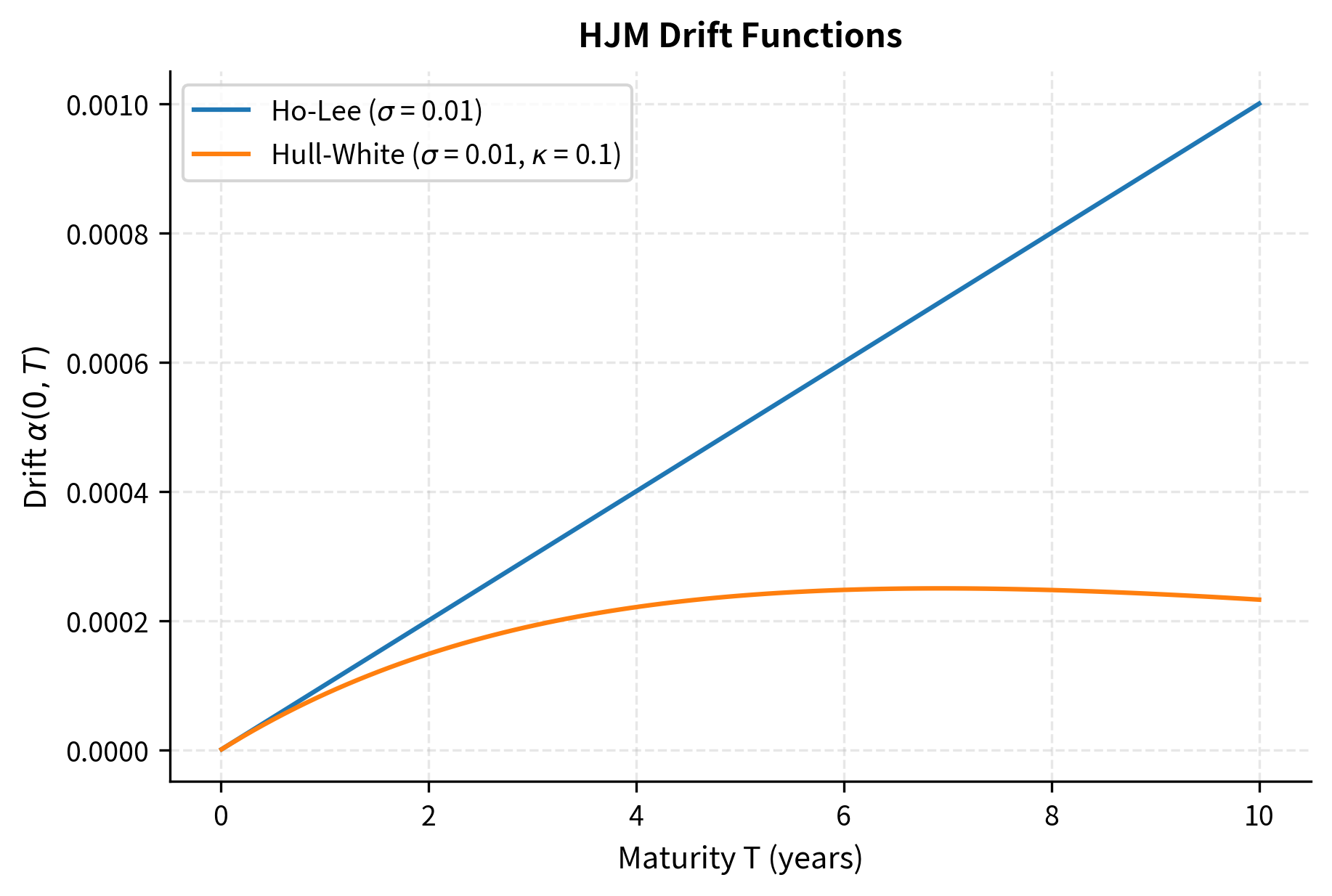
The Ho-Lee drift grows without bound as maturity increases, which can lead to unrealistic long-term behavior. Forward rates at very long maturities would drift upward at an accelerating pace, potentially reaching implausibly high levels. The Hull-White specification, with its exponentially decaying volatility, produces a bounded drift that stabilizes at longer maturities. This behavior aligns better with economic intuition: long-term rates should not exhibit explosive dynamics.
Simulating Forward Rate Curves Under HJM
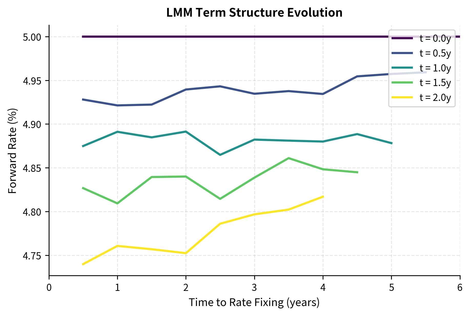
To implement HJM in practice, we discretize time and simulate the forward rate curve evolution. Starting from today's observed forward curve , we evolve each point on the curve simultaneously. This parallel evolution captures how the entire term structure moves together while respecting the no-arbitrage constraint. The simulation proceeds by applying small increments to each forward rate, with the drift determined by the HJM condition and the random shock drawn from a standard normal distribution scaled by the volatility function.
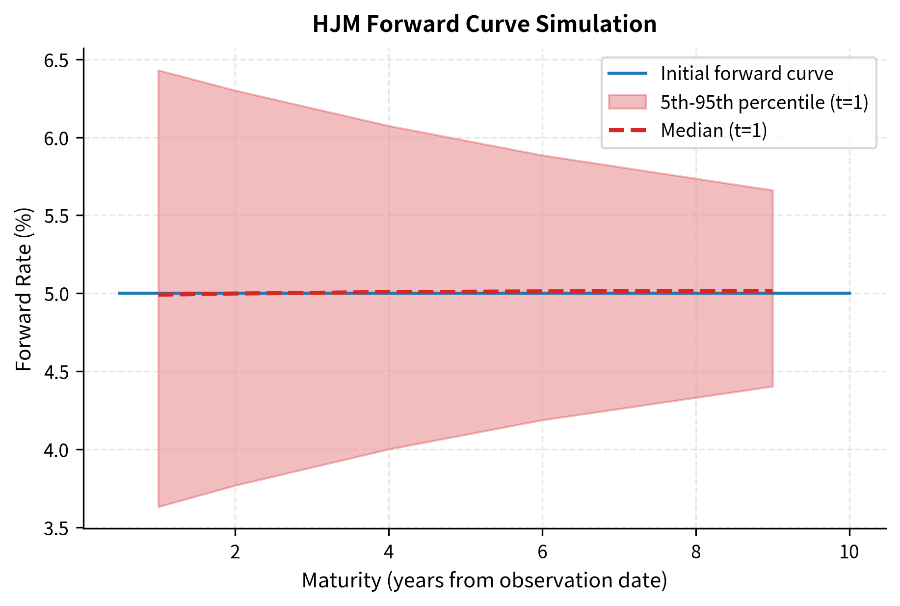
The simulation shows how the forward rate curve evolves over time under HJM dynamics. The initial flat curve develops both level shifts and changes in shape, with uncertainty increasing over the simulation horizon. The widening confidence band reflects the accumulation of random shocks over time, while the upward drift of the median reflects the convexity adjustment built into the HJM drift condition. Note that as time passes, short-maturity rates "expire" and are no longer meaningful, which is why we shift the maturities when plotting the future distribution.
Key Parameters
The key parameters for the HJM framework simulations are:
- f(0, T): Initial forward rate curve. The starting point for the evolution of the term structure, typically extracted from market bond prices or swap rates.
- σ(t, T): Volatility function. Determines the magnitude of random fluctuations and, via the drift condition, the trend of forward rates. This is the sole input needed to specify an HJM model.
- κ: Mean reversion parameter (in Hull-White specification). Controls how quickly volatility decays with maturity, influencing the correlation between forward rates of different tenors.
- dt: Time step size. Smaller steps reduce discretization error in the simulation but increase computational cost.
The LIBOR Market Model
While the HJM framework provides a theoretically elegant approach to modeling forward rates, it works with instantaneous forward rates, which are not directly observable in markets. You cannot go to a broker and ask to trade the instantaneous forward rate for borrowing at exactly 2.5 years from now. You price caps, floors, and swaptions using discrete forward LIBOR rates for specific tenors (3-month, 6-month). The LIBOR Market Model (LMM), also known as the Brace-Gatarek-Musiela (BGM) model, directly models these market-observable rates. This alignment with market conventions makes LMM the natural choice for pricing and hedging interest rate derivatives.
Forward LIBOR Rates
Consider a set of tenor dates with equal spacing (typically 0.25 or 0.5 years). The forward LIBOR rate is the simply compounded rate at time for borrowing over the period . Unlike the continuously compounded instantaneous forward rate in HJM, the LIBOR rate applies simple interest over a discrete period:
where:
- : year fraction (accrual period)
- : price of a zero-coupon bond maturing at
- : price of a zero-coupon bond maturing at
The formula expresses a simple arbitrage relationship: if you invest one dollar at the LIBOR rate from to , you should receive dollars. Alternatively, you could buy bonds maturing at , which costs in terms of bonds maturing at . Equating these two strategies yields the formula above.
These rates are directly observable from the forward rate agreement (FRA) market and serve as the underlying rates for caps and floors. When a bank quotes a 6-month LIBOR rate starting in 1 year, that is exactly the forward rate for the appropriate index .
LMM Dynamics Under the Forward Measure
The key insight of LMM is that under the -forward measure , the forward LIBOR rate is a martingale. This follows because can be expressed as a ratio of asset prices (zero-coupon bonds), and ratios of tradeable assets are martingales under the numeraire corresponding to the denominator. This is a direct application of the change of numeraire theorem. When we use as the numeraire, any asset price divided by this numeraire becomes a martingale, and the forward rate is precisely such a ratio.
Under this forward measure, has zero drift and follows:
where:
- : volatility of the -th forward rate
- : Brownian motion under the -forward measure
The lognormal dynamics implied by this equation have profound practical consequences. Because the rate follows geometric Brownian motion under its natural measure, its distribution at any future time is lognormal. This lognormal distribution leads directly to Black's formula for caplet pricing, providing the theoretical justification for the market convention that predated the formal LMM framework.
The -forward measure uses the zero-coupon bond as numeraire. Under this measure, any asset price divided by is a martingale. The forward LIBOR rate is naturally a martingale under the -forward measure.
Black's Formula for Caplets
A caplet pays at time , where is the cap rate. This payoff represents the protection provided by the cap: if the realized LIBOR rate exceeds the cap strike, the holder receives the difference applied to the notional over the accrual period. Since is a martingale under and follows lognormal dynamics, the caplet price has a Black-Scholes-type closed-form solution known as Black's formula:
where:
- : initial forward LIBOR rate
- : cap strike rate
- : discount factor for the payment date
- : cumulative standard normal distribution function
- : integrated volatility (approximated as for constant volatility)
The formula terms provide the following intuition:
- : probability that the option expires in-the-money under the forward measure
- : expected value of the floating rate at maturity, conditional on exercise
- : expected cost of the fixed rate strike payment, conditional on exercise
The structure mirrors the Black-Scholes formula for equity options, which is no coincidence. Both arise from the same mathematical setting: lognormal dynamics under the relevant pricing measure. The discount factor converts the expected payoff under the forward measure to a present value.
A cap is simply a portfolio of caplets:
where:
- Cap: total value of the interest rate cap
- Caplet_i: value of the -th individual caplet
- : number of caplets in the contract
Each caplet in the cap protects against high rates in a different future period, and since the caplets have non-overlapping payoff dates, they can be valued independently and summed.
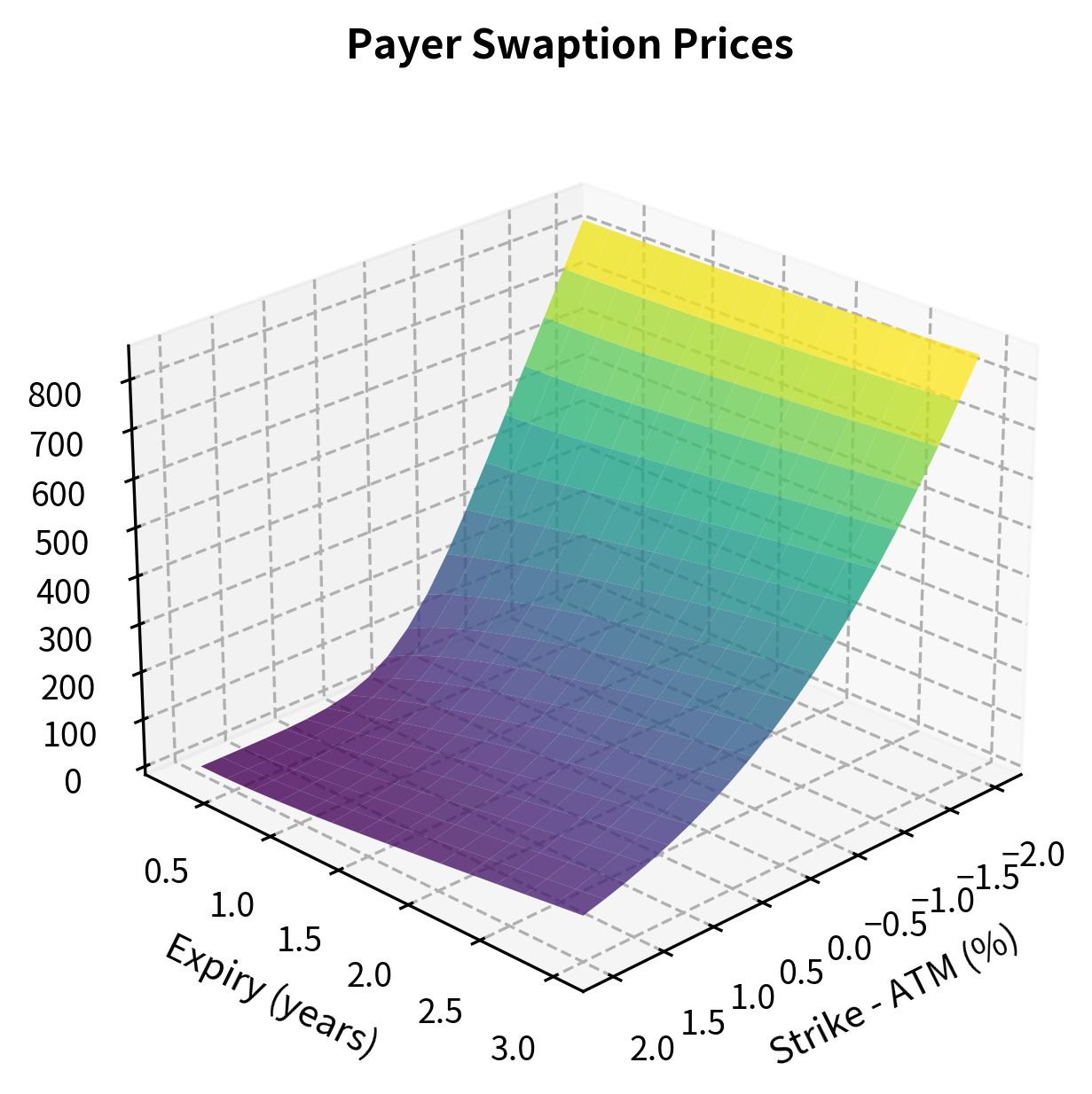
The cap price of approximately 1.77% of notional represents the premium required to hedge against floating rates exceeding 5% over the next 3 years. This value reflects the sum of individual caplet prices, each weighted by the discount factor and the probability of the forward rate exceeding the strike. For an at-the-money cap where the strike equals the forward rate, roughly half of the value comes from intrinsic value considerations and half from time value.

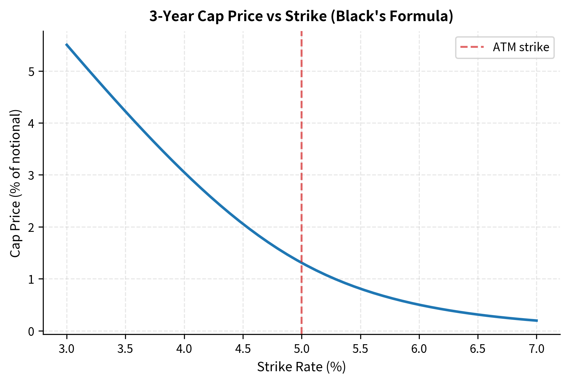
The plot illustrates the inverse relationship between cap prices and strike rates. As the strike increases, the cap becomes more out-of-the-money, reducing its value. A higher strike means the cap provides protection only against more extreme rate increases, which are less likely to occur. The curvature reflects the non-linear nature of option pricing with respect to the strike, with the steepest gradient occurring near the at-the-money rate where the option's moneyness is most sensitive to small changes in the strike.
LMM Dynamics Under the Terminal Measure
While Black's formula works beautifully for individual caplets, pricing more complex derivatives like swaptions requires simulating multiple forward rates simultaneously. The challenge is that each forward rate is a martingale under a different measure . We cannot simply simulate each rate as a driftless process because they all need to evolve consistently under the same probability measure.
To simulate all rates consistently, we typically work under a single measure, commonly the terminal measure (using as numeraire). Under this measure, only is a driftless martingale. Other forward rates acquire drift terms that arise from the change of measure between their natural measures and the terminal measure.
Under , the dynamics of for become:
where:
- : forward LIBOR rate
- : drift term under the terminal measure
- : volatility of the forward rate
- : Brownian motion under the terminal measure
The drift term is defined as:
where:
- : forward LIBOR rates
- : accrual period
- : correlation between forward rates and
- : volatilities of the respective forward rates
- : state-dependent drift ensuring no arbitrage under the terminal measure
This drift term ensures consistency when modeling all rates under the single terminal measure . To understand each component, consider the following interpretation. The fraction measures the sensitivity of the bond price ratio to the rate . This is essentially the duration of a single-period bond with respect to its yield. The product captures the covariance between the rate being modeled () and the rates acting as numeraires (). The summation accumulates adjustments for all intermediate rates between the payment date and the terminal horizon.
This drift term arises from the change of measure from each forward rate's natural measure to the terminal measure. The negative sign indicates that rates with earlier payment dates tend to drift downward under the terminal measure, which compensates for the fact that they are martingales under different measures.
Correlation Structure
The correlation structure between forward rates is crucial for pricing products that depend on multiple rates (like swaptions). A swap rate is essentially a weighted average of forward rates, so the volatility of the swap rate depends not just on the individual forward rate volatilities but also on how the forward rates co-move. Common parameterizations include:
Constant correlation:
where:
- : correlation between forward rates and
- : constant correlation parameter
This simple specification assumes that all pairs of forward rates have the same correlation. While convenient for calibration, it lacks economic nuance because it treats the correlation between 1-year and 2-year rates the same as the correlation between 1-year and 10-year rates.
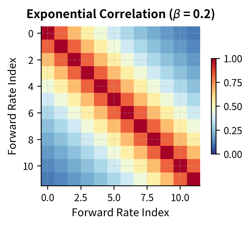
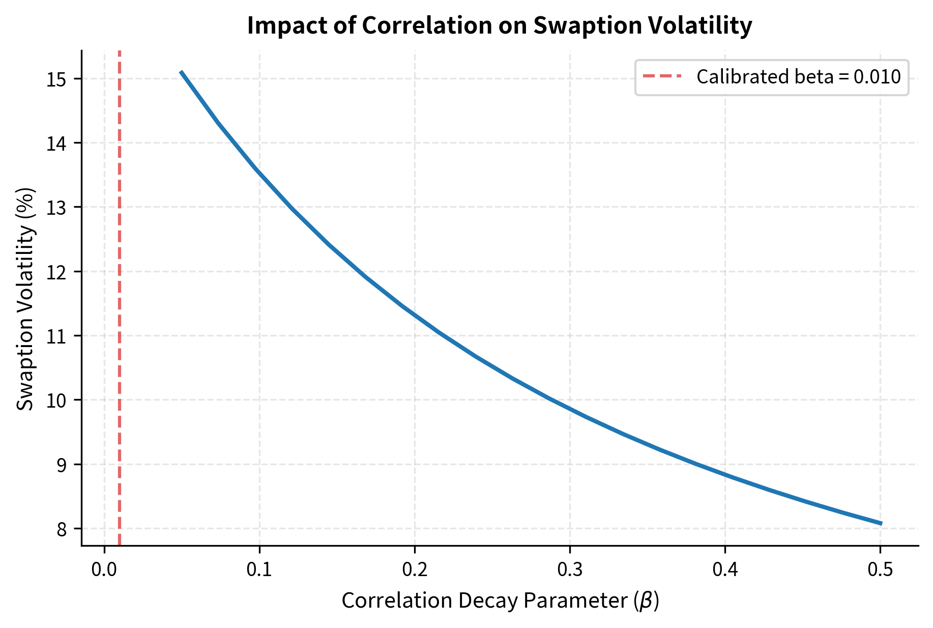
Exponential decay:
where:
- : correlation decay parameter
- : distance between tenor indices
This captures the intuition that forward rates with similar maturities are more correlated than rates far apart. Economic factors that drive short-term rates (monetary policy, near-term economic outlook) differ from those driving long-term rates (inflation expectations, long-run growth potential). The exponential form provides a smooth transition from high correlation for adjacent rates to lower correlation for distant rates.

Monte Carlo Simulation of the LMM
To price complex derivatives under the LMM, we simulate forward rate paths using the discretized dynamics under the terminal measure. The simulation requires careful handling of the state-dependent drift: at each time step, we must first evaluate the current drift based on the current forward rates before updating the rates for the next step. This creates a natural ordering where we update rates from longest maturity to shortest, since shorter rates depend on longer rates through the drift formula.
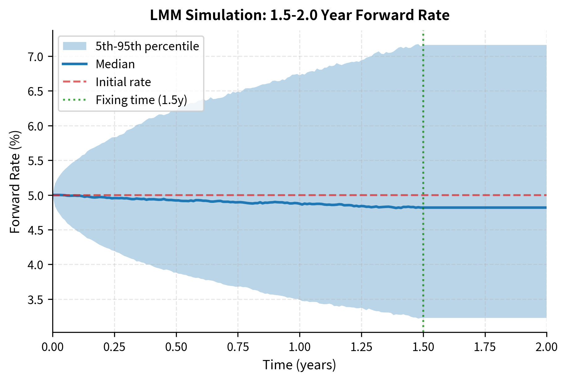
The simulation captures the stochastic evolution of forward rates, including their correlation structure. Notice how the rate fixes at its fixing time and remains constant thereafter. Before the fixing time, the rate fluctuates randomly around its initial value, with the distribution widening as time progresses. After fixing, the rate becomes a realized constant, which reflects the actual market mechanics where LIBOR rates are set at the beginning of each accrual period.
Key Parameters
The key parameters for the LIBOR Market Model are:
- L_i(0): Initial forward LIBOR rates. Observable directly from the current yield curve, these provide the starting point for all simulations and ensure the model fits today's market prices exactly.
- σ_i: Volatility of the i-th forward rate. Determines the width of the distribution for each rate and is typically calibrated to cap volatility data.
- ρ_ij: Correlation between forward rates L_i and L_j. Crucial for pricing multi-rate products like swaptions, as it determines how the rates co-move and thus affects the volatility of rate combinations.
- δ: Accrual period (tenor spacing). Typically 0.25 (3 months) or 0.5 (6 months), matching the conventions of the underlying interest rate contracts.
- β: Correlation decay parameter. Controls how quickly correlation decreases as the distance between rate maturities increases, with higher values producing faster decay.
Swaption Pricing Under the LMM
A swaption is an option to enter into an interest rate swap at a future date. A payer swaption gives you the right to pay fixed and receive floating, while a receiver swaption gives the right to receive fixed and pay floating. Swaptions are among the most liquid interest rate derivatives and are crucial for calibrating the LMM. Their prices reflect market expectations about both the level and volatility of future interest rates, making them valuable sources of information for model calibration.
Swap Rate and Swaption Payoff
The forward swap rate for a swap starting at and ending at is the fixed rate that makes the swap have zero value at inception. It can be expressed as the ratio of two present values:
where:
- : price of bond maturing at swap start date
- : price of bond maturing at swap end date
- : present value of the fixed leg's annuity factor (PVBP)
The numerator represents the present value of receiving one dollar at the swap start and paying one dollar at the swap end. This is exactly the floating leg's present value for a swap with a notional of one dollar. The denominator, the annuity factor, represents the present value of receiving one dollar at each payment date. The ratio therefore gives the fixed rate that equates the present values of the fixed and floating legs.
A payer swaption with strike has payoff at expiry :
where:
- : annuity factor at expiry
- : forward swap rate at expiry
- : swaption strike rate
The payoff structure reflects that exercising a payer swaption is valuable when the market swap rate exceeds the strike: you can immediately enter a swap paying below-market rates. The multiplication by the annuity factor converts the rate difference into a present value, accounting for all future payment dates.
Swaption Approximation Formula
While the swap rate under LMM does not follow exactly lognormal dynamics (it's a function of multiple forward rates), a common approximation assumes lognormal swap rate dynamics. This approximation is remarkably accurate in practice because the swap rate, being a weighted average of forward rates, tends toward normality by the central limit theorem and the log of a sum is approximately the sum of logs when the rates are similar in magnitude. This leads to Black's formula for swaptions:
where:
- : initial annuity factor
- : initial forward swap rate
- : swaption strike rate
- : total swaption volatility ()
As with the caplet formula, this expression decomposes the value into interpretable components:
- is the expected value of the floating leg conditional on exercise
- is the expected value of the fixed leg conditional on exercise
- The annuity factor discounts the future swap cash flows to a present lump sum
Since the swap rate behaves approximately as a weighted average of the forward rates, its variance can be derived from the covariances of the underlying forward rates. This is a direct application of the formula for the variance of a linear combination of random variables. The total swaption volatility squared is approximated by:
where:
- : weights representing the elasticity of the swap rate with respect to each forward rate
- : correlation between forward rates
- : volatility of forward rate
- : time to swaption expiry
The weights measure how sensitive the swap rate is to each underlying forward rate. These weights sum to one (approximately) and tend to be larger for rates near the middle of the swap than for rates at the ends. The double summation captures both the variance contributions from each rate (when ) and the covariance contributions from pairs of rates (when ).
The payer swaption price of approximately 1726 basis points represents the upfront premium required to purchase the right to pay 5% fixed on the swap. This value is derived from the volatility of the swap rate and the time to expiry. For context, this means that on a notional of \$100 million, the swaption would cost approximately \$1.726 million. The relatively high price reflects both the long tenor of the underlying swap and the substantial uncertainty about interest rates over the one-year option period.
Monte Carlo Swaption Pricing
For more accurate pricing that captures the correlation structure, we can use Monte Carlo simulation under the LMM. This approach simulates the joint evolution of all forward rates, calculates the swap rate at expiry from the simulated rates, and averages the discounted payoffs across all paths. The Monte Carlo method naturally handles the complex dependence of the swap rate on multiple forward rates without requiring the approximations used in the analytical formula.
The Monte Carlo price should be close to Black's formula for ATM options. Differences arise from the approximation in Black's formula and simulation noise. The standard error provides a measure of the Monte Carlo estimation uncertainty: with 5000 paths, we achieve reasonable precision, but production implementations often use many more paths combined with variance reduction techniques to achieve tighter confidence intervals.
Key Parameters
The key parameters for swaption pricing are:
- S: Forward swap rate. The par rate that sets the swap's initial value to zero, observable from the current yield curve.
- K: Strike rate. The fixed rate specified in the swaption contract, chosen at inception and remaining fixed throughout the option's life.
- A: Annuity factor. The present value of the fixed leg's basis point payments, which converts rate differences into dollar values.
- T: Time to expiry. The time until the option is exercised, during which the swap rate may move in favor of or against the option holder.
- σ: Swaption volatility. The volatility of the forward swap rate used in Black's formula, typically implied from market prices.
Calibration to Market Data
Calibration is the process of choosing model parameters (volatilities, correlations) so that the model reproduces observed market prices. For interest rate models, calibration typically targets cap/floor volatilities and swaption volatilities. The goal is to find parameters that allow the model to price liquid instruments consistently with the market while maintaining reasonable behavior for illiquid or exotic instruments. This balancing act is central to practical derivatives pricing.
Cap Volatility Calibration
Market caps are quoted in terms of implied volatility. Given a quoted cap volatility, we can back out the price using Black's formula, then calibrate the LMM volatilities to match these prices. The calibration process inverts the pricing formula: rather than using volatility to find price, we use price to find volatility.
The caplet volatility structure in LMM has several common parameterizations. A popular choice is the piecewise-constant volatility, where each forward rate has a constant volatility that can differ across maturities. More sophisticated approaches use time-varying or maturity-dependent volatility functions that can capture features like the volatility "hump" often observed at intermediate maturities.
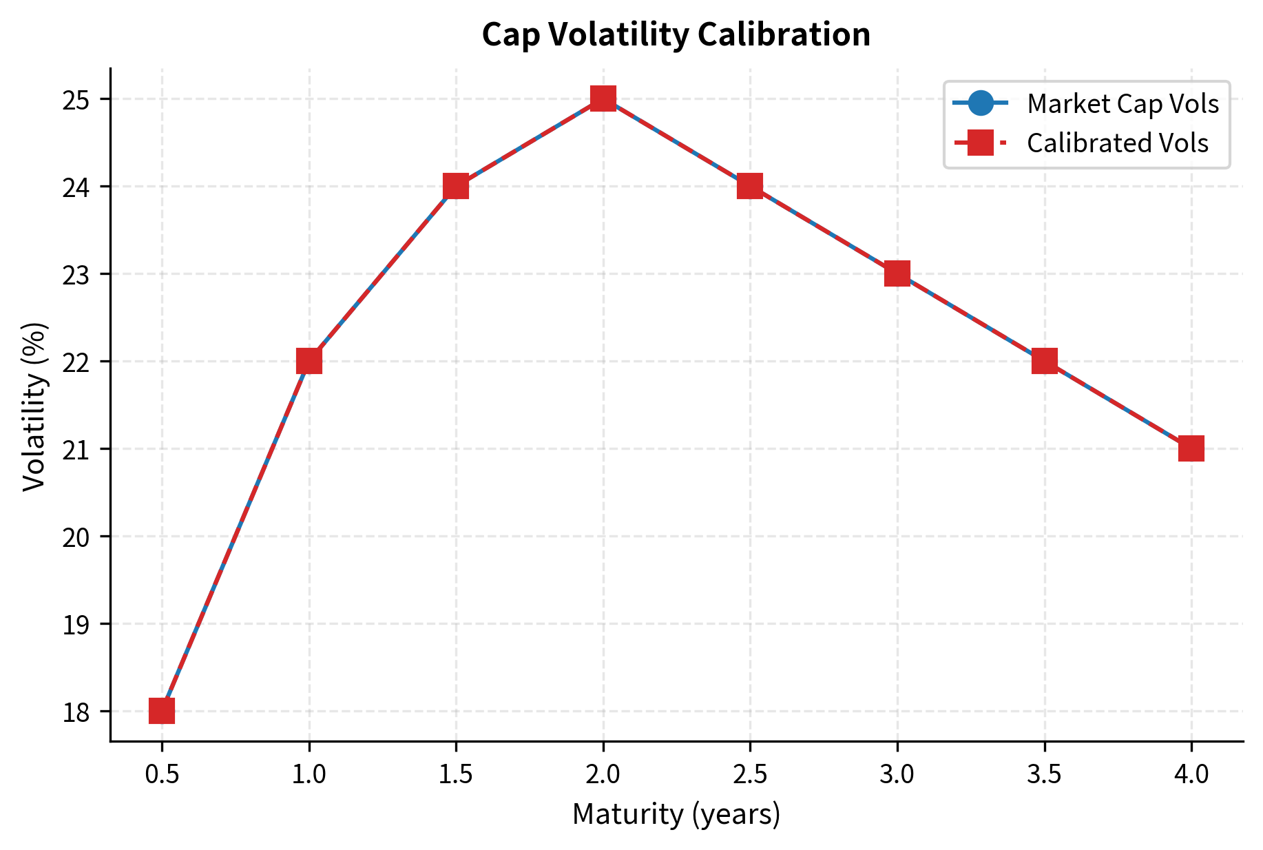
The calibration results demonstrate the model's ability to fit the term structure of volatility. The calibrated forward rate volatilities track the market cap volatilities, capturing the hump shape around the 2-year mark that is characteristic of interest rate markets. This hump reflects the market's view that rates are most uncertain at intermediate horizons: near-term rates are anchored by current monetary policy, while very long-term rates are stabilized by mean reversion.
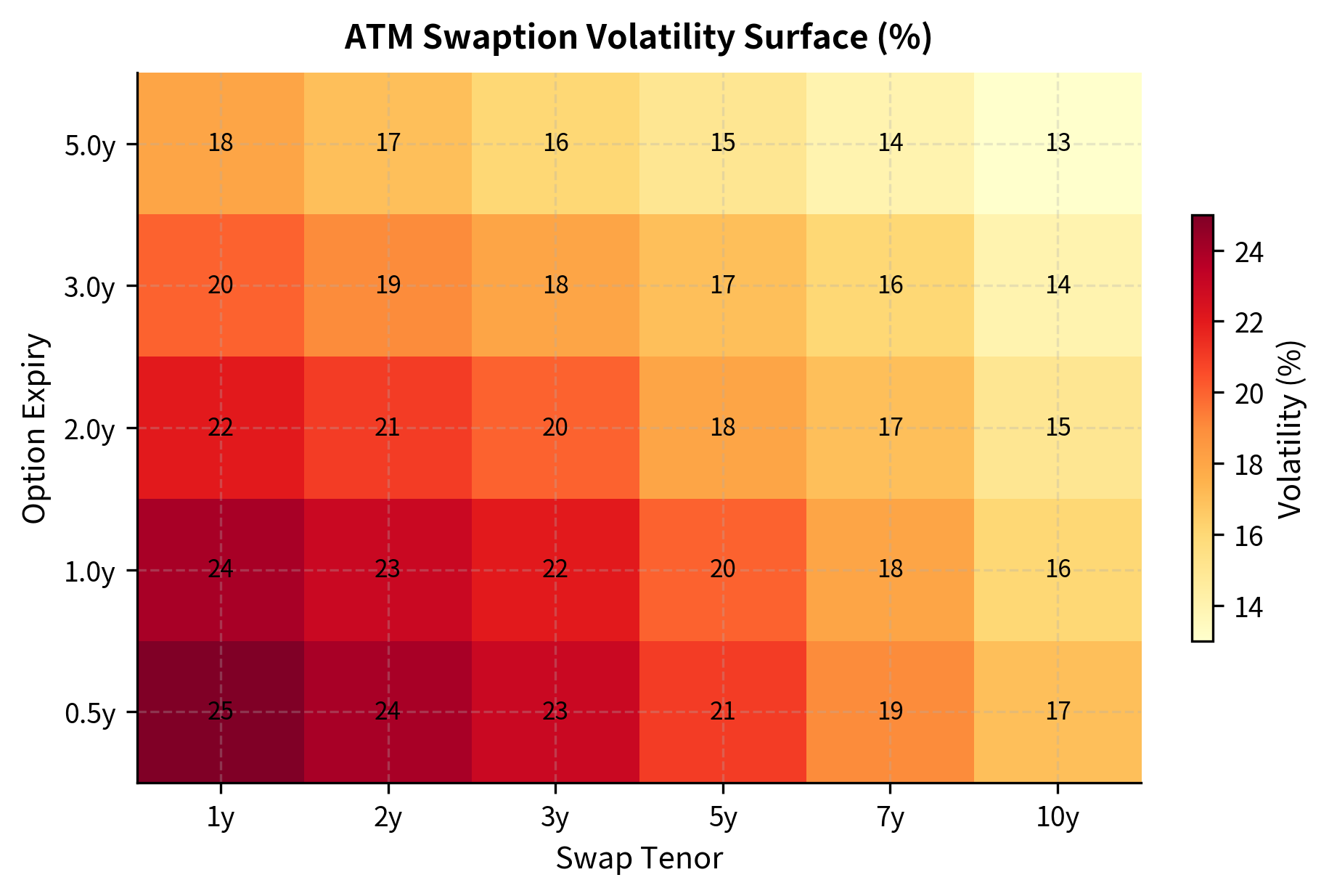
Swaption Volatility Surface Calibration
The swaption market provides a rich volatility surface across different expiries and swap tenors. Calibrating the LMM to this surface is more challenging because swaption volatility depends on both individual forward rate volatilities and their correlations. Unlike cap calibration, where each caplet can be calibrated independently, swaption calibration requires simultaneously fitting multiple interdependent parameters.
A typical swaption volatility surface (often called a "vol cube" when strikes are included) shows variation across:
- Expiry: Time until the option expires
- Tenor: Length of the underlying swap
- Strike: Often expressed as offset from ATM

Joint Calibration Challenge
Calibrating the LMM to both caps and swaptions simultaneously is challenging because caps constrain individual forward rate volatilities while swaptions constrain both volatilities and correlations. A model that fits cap volatilities perfectly may still misprice swaptions if the correlation structure is wrong. Conversely, adjusting correlations to fit swaptions may introduce inconsistencies with cap prices. A common approach involves:
- Stage 1: Calibrate forward rate volatilities to the cap volatility curve
- Stage 2: Calibrate correlations to match swaption volatilities, given the volatilities from Stage 1
More sophisticated approaches use global optimization to calibrate volatilities and correlations jointly, treating the entire parameter set as a single optimization problem. This avoids the suboptimality that can arise from sequential calibration but requires more computational resources and careful attention to the objective function weighting.
The calibration shows that while we can match some swaptions well, perfect fit across the entire surface requires more sophisticated volatility and correlation parameterizations. This is an active area of research and practical development. In production systems, you often use more flexible correlation structures (such as angle-based parameterizations) and volatility functions that depend on both time and maturity to achieve better fits.
Practical Implementation Considerations
Implementing HJM and LMM in production systems involves several practical challenges that go beyond the theoretical framework. The gap between textbook models and real trading systems requires careful attention to numerical issues, computational efficiency, and evolving market conventions.
Numerical Stability
The lognormal dynamics in LMM can occasionally produce negative forward rates in extreme scenarios due to discretization errors. When simulating over long horizons or with large time steps, the Euler discretization may produce values that violate the theoretical positivity constraint. Common remedies include:
- Using shifted lognormal dynamics , where is a shift parameter. This approach handles negative rates gracefully and has become standard practice in the post-2008 low-rate environment.
- Employing predictor-corrector schemes for more accurate discretization. These methods use an initial estimate (predictor) and refine it (corrector) to achieve better accuracy than simple Euler steps.
- Implementing floor constraints to prevent negative rates. While computationally simple, this approach can introduce bias in the simulation.
Computational Efficiency
Monte Carlo simulation of the LMM is computationally intensive, especially for large books of derivatives. Each derivative may require thousands of paths, and a trading desk may need to price thousands of derivatives daily for risk management. You employ various techniques to accelerate calculations:
- Variance reduction: Antithetic variates, control variates, and importance sampling (as covered in our chapter on Monte Carlo methods) can dramatically reduce the number of paths needed for a given accuracy level.
- Parallel computing: Simulating paths independently on multiple processors. Modern implementations leverage GPUs, which can simulate thousands of paths simultaneously.
- Low-discrepancy sequences: Quasi-Monte Carlo methods for faster convergence. These deterministic sequences fill the sample space more uniformly than random sampling, often achieving convergence rates better than the rate of standard Monte Carlo.
Post-LIBOR Considerations
Following the LIBOR transition, the market has largely shifted to risk-free rates (RFR) such as SOFR, SONIA, and €STR. The LMM framework has been adapted to model these rates, though the mechanics differ somewhat because RFRs are typically compounded in arrears rather than set in advance. Unlike LIBOR, which was a forward-looking term rate fixed at the beginning of the accrual period, RFR-based rates compound daily observations over the accrual period. This mechanical difference affects hedging strategies and requires modifications to the simulation framework. The fundamental mathematical structure of forward rate modeling remains applicable, but calibration targets and market conventions have evolved.
Comparison: Short-Rate Models vs. HJM vs. LMM
Understanding when to use each modeling approach is crucial for you. This table summarizes the key trade-offs:
| Aspect | Short-Rate Models | HJM Framework | LIBOR Market Model |
|---|---|---|---|
| Primary variable | Instantaneous short rate | Instantaneous forward curve | Discrete forward rates |
| Yield curve fit | Requires affine term structure or calibration | Built-in by construction | Built-in by construction |
| Cap/Floor pricing | Approximations needed | Possible but complex | Black's formula exact |
| Swaption pricing | Closed-form for some models | Complex | Approximation or MC |
| Calibration difficulty | Moderate | High | Moderate to High |
| Use cases | Bond pricing, simple derivatives | Theoretical, exotic derivatives | Caps, floors, swaptions |
Short-rate models remain valuable for their analytical tractability and are often used for ALM (Asset-Liability Management) and bond portfolio management. Their simplicity makes them suitable for applications where detailed calibration to derivative prices is less important than capturing the general dynamics of interest rate movements. The HJM framework provides deep theoretical insights and is the foundation for more complex models. Its generality makes it the natural starting point for understanding arbitrage-free term structure evolution. The LMM has become the industry standard for pricing and hedging interest rate derivatives because it directly models the rates used in these products, providing a natural connection between model variables and market observables.
Limitations and Impact
The HJM and LMM frameworks transformed interest rate derivatives pricing by providing a consistent framework for modeling forward rates that automatically fits the current yield curve. Before these models, we struggled to reconcile model-implied rates with market observations, leading to pricing inconsistencies and hedging errors. HJM established that in an arbitrage-free economy, the drift of forward rates is completely determined by their volatility structure, unifying different modeling approaches.
However, these frameworks come with significant limitations. The HJM framework, while theoretically elegant, can lead to non-Markovian dynamics that are difficult to implement efficiently. The general HJM model may require tracking the entire history of rate evolution, making computational methods memory-intensive. The LMM, designed to address this by working with observable rates, introduces its own challenges. The drift terms under a common measure involve all forward rates, creating path-dependent dynamics that require Monte Carlo simulation for most products beyond vanilla caps.
Both frameworks face challenges in capturing real market behavior. The assumption of lognormal forward rate dynamics produces constant volatility for caplets, yet markets display pronounced volatility smiles and skews. Extensions like stochastic volatility and local volatility modifications address this but add significant model complexity. Calibration to the full swaption volatility surface often reveals tension between fitting individual instruments and maintaining sensible model behavior. A model perfectly calibrated to today's prices may produce unstable hedges or unrealistic forward dynamics.
The correlation structure in LMM deserves particular attention. While we can parameterize correlations to fit observed swaption prices, the resulting correlation matrices may not reflect actual rate co-movements, particularly during market stress. The 2008 financial crisis and subsequent market dislocations revealed that correlation structures estimated from normal markets can break down precisely when they matter most for risk management.
Looking ahead, the next chapter on valuation of interest rate derivatives will apply these frameworks to price specific products including Bermudan swaptions, callable bonds, and structured notes. The calibration techniques introduced here will be developed more formally in our later chapter on calibration and parameter estimation, where we'll explore global optimization methods and assess model risk.
Summary
This chapter developed two foundational frameworks for advanced interest rate modeling. The Heath-Jarrow-Morton approach models the evolution of the entire instantaneous forward rate curve, with the crucial insight that absence of arbitrage completely determines the forward rate drift in terms of its volatility structure. This drift condition, , ensures that discounted bond prices are martingales under the risk-neutral measure.
The LIBOR Market Model takes a more practical approach by directly modeling discrete forward rates observable in the market. Under each forward rate's natural measure, the rate follows driftless lognormal dynamics, leading directly to Black's formula for caplet pricing. Simulating multiple rates requires working under a common measure, introducing drift terms that depend on the correlation structure.
Key implementation concepts include:
- Forward measure numeraire: The bond serves as numeraire under the -forward measure, making the corresponding forward rate a martingale
- Black's formula: Provides closed-form caplet and floorlet prices under lognormal forward rate assumptions
- Correlation parameterization: Exponential decay structures capture the intuition that adjacent forward rates are more correlated than distant ones
- Two-stage calibration: First fit cap volatilities, then calibrate correlations to swaption prices
The frameworks balance flexibility with tractability. While they can match observed market prices more accurately than short-rate models, they require careful attention to numerical implementation, particularly for Monte Carlo simulation. Modern implementations often extend these basic frameworks with stochastic volatility or local volatility modifications to capture smile dynamics observed in the market.
Quiz
Ready to test your understanding? Take this quick quiz to reinforce what you've learned about the Heath-Jarrow-Morton framework and LIBOR Market Model.

Comments