

Master Black's model for pricing interest rate options. Learn to value caps, floors, and swaptions with Python implementations and risk measures.
Choose your expertise level to adjust how many terms are explained. Beginners see more tooltips, experts see fewer to maintain reading flow. Hover over underlined terms for instant definitions.
Valuation of Interest Rate Derivatives
Interest rate derivatives represent one of the largest and most liquid segments of the global derivatives market, with notional amounts outstanding in the hundreds of trillions of dollars. While we explored the mechanics and valuation of interest rate swaps in Part II, we often need more than just the ability to lock in fixed rates. You need options: the right, but not the obligation, to enter into interest rate contracts or to receive payments when rates move beyond certain thresholds.
This chapter brings together the option pricing frameworks from earlier chapters with the interest rate modeling techniques from Chapters 14 and 15. We'll see how Black's model, a close relative of the Black-Scholes framework, provides the market standard for pricing caps, floors, and swaptions. Understanding these instruments is essential for you in fixed income markets, whether you are managing corporate debt, structuring mortgage products, or running a trading desk.
Interest Rate Options: The Big Picture
Interest rate derivatives give you asymmetric payoffs based on interest rate movements. Unlike swaps, which create symmetric obligations for both parties, options allow one party to benefit from favorable rate movements while limiting downside exposure.
The three primary categories of interest rate options are:
- Caps and Floors: Options that provide protection against rates rising above (cap) or falling below (floor) a specified strike level
- Swaptions: Options to enter into an interest rate swap at a future date with pre-specified terms
- Bond Options: Options on specific bonds or bond futures, often embedded in callable or putable bonds
These instruments serve both hedging and speculative purposes. You might purchase a cap to limit maximum interest expenses on floating-rate debt, or use swaptions to hedge the prepayment risk embedded in a mortgage portfolio. You might also trade volatility by buying or selling caps and swaptions based on views about future rate volatility.
Caps and Floors
A cap is a portfolio of interest rate call options, each called a caplet, that provides you with payments whenever a reference rate exceeds a predetermined strike rate. A floor is the corresponding portfolio of put options, called floorlets, that pays when the reference rate falls below the strike. Understanding how these instruments work requires us to first examine the building blocks, namely individual caplets and floorlets, before assembling them into complete cap and floor structures.
Caplet and Floorlet Mechanics
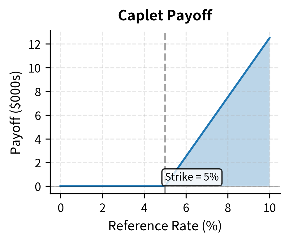
To understand how caplets work, consider that you are a borrower with floating-rate debt who worries about rising interest rates. Each quarter, your interest payment resets based on market rates. If rates spike unexpectedly, you face a sudden increase in interest expense. A caplet provides insurance against exactly this scenario: it pays you whenever the market rate exceeds a predetermined ceiling.
Consider a caplet that settles at time based on the interest rate observed at time . The timing distinction matters here: the rate is determined, or "fixed," at , but the actual payment occurs at , typically three or six months later. This structure mirrors how floating-rate loans work, where the rate for each period is set at the beginning but interest is paid at the end. If the reference rate (typically a LIBOR or SOFR rate) exceeds the strike rate , you receive a payment. The payment occurs at and equals:
where:
- : notional principal
- : day count fraction between and
- : reference interest rate (e.g., LIBOR or SOFR) observed at time
- : strike rate
Notice how the payoff is structured. The term ensures the payment is never negative: when rates are below the strike, the caplet simply expires worthless, and you owe nothing. When rates exceed the strike, you receive the difference. The notional principal and day count fraction convert this rate difference into an actual dollar amount, following the same conventions used in the underlying floating-rate loan.
The caplet payoff looks exactly like a call option on an interest rate. Just as a stock call option pays the excess of the stock price over the strike, a caplet pays the excess of the interest rate over the strike rate. This allows us to adapt option pricing theory to interest rates.
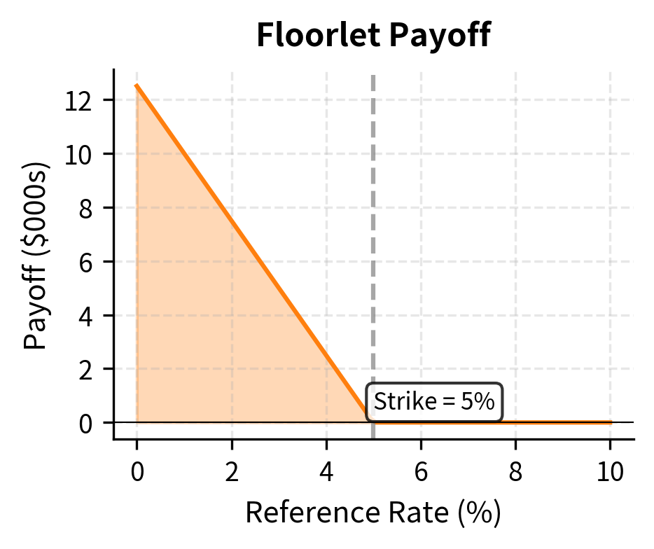
The floorlet payoff follows the same structure but uses a put option:
where:
- : notional principal
- : day count fraction
- : strike rate
- : reference interest rate
A floorlet protects against falling rates rather than rising rates. Consider that you have made fixed-rate loans funded by floating-rate deposits. If rates fall, you continue receiving fixed payments from borrowers but pay less on deposits, which is favorable. However, if rates rise, the opposite occurs. A floorlet provides the mirror-image protection to a cap, paying you when rates fall below the strike level.
A cap consists of multiple caplets covering consecutive periods. For example, a 3-year cap on quarterly rates would contain 12 caplets, one for each quarter. The first caplet typically starts at the first reset date (often 3 or 6 months from inception), which means the first fixing is already known at inception and the corresponding caplet has no optionality. This first caplet is often called the "stub" period, and market conventions vary on whether it is included in the quoted cap price.
Black's Model for Caplet Pricing
To value these payments, we use Black's model, an extension of the Black-Scholes framework.
Black's model treats the forward rate for each period as the underlying asset. Rather than modeling how interest rates evolve continuously over time, Black's approach takes the forward rate as given and asks: what is the fair price for an option on this forward rate?
To make this approach work, Black's model assumes the forward rate for each period follows a lognormal distribution under a specific probability measure, known as the forward measure associated with that period's payment date. The lognormal assumption means that forward rates are always positive and that percentage changes in rates are normally distributed. While this assumption has limitations, particularly when rates are near zero, it provides tractable closed-form solutions that form the foundation of market practice.
Under Black's model, the price of a caplet paying at time based on the rate set at is:
where:
- : notional principal
- : day count fraction
- : today's discount factor to time
- : forward rate from to
- : strike rate
- : cumulative standard normal distribution function
- : volatility of the forward rate
- : time to rate fixing
- : measures how many standard deviations the forward rate is above the strike, adjusted for time and volatility
- : a risk-adjusted measure accounting for volatility over the time to fixing
- : expected value of the forward rate, conditional on the option being in-the-money
- : strike rate weighted by the probability of exercise
Let's carefully unpack each component of this formula to build intuition for why it takes this form.
The term outside the brackets converts the rate-based payoff into a present value. The notional and day count fraction translate a rate difference into a cash amount, while the discount factor brings this future cash payment back to today's dollars. Notice that we discount to the payment date , not the fixing date , because that is when cash actually changes hands.
Inside the brackets, we find the familiar Black-Scholes structure adapted to forward rates. The term represents the expected payoff from the forward rate component, weighted by the probability that the option finishes in the money (after a specific risk adjustment). The term represents what we expect to "give up" by paying the strike, again weighted by exercise probability. The difference between these two terms gives the option's expected payoff under the forward measure.
The formula closely resembles the Black-Scholes formula from Chapter 6, with key differences. The underlying is a forward rate rather than a stock price, and the discount factor appears outside the main expression rather than being embedded through a risk-free rate term. The time to expiration is , the rate-setting date, not , the payment date. This distinction is critical: the option's uncertainty resolves when the rate is fixed, even though the payment comes later.
The parameters and measure how far the forward rate sits from the strike in standardized units. When equals , the caplet is at-the-money, and and depend only on volatility and time. When exceeds , the forward rate is above the strike, making the caplet in-the-money and increasing both and . The volatility parameter captures how uncertain we are about where the forward rate will settle by the fixing date. Higher volatility means more dispersion, which increases option value because you benefit from upside while being protected from downside.
For floorlets, the pricing formula uses the put option version:
where:
- : notional principal
- : day count fraction
- : discount factor to time
- : forward rate
- : strike rate
- : volatility of the forward rate
- : probabilities associated with the put option calculation
The floorlet formula mirrors the caplet formula with the roles reversed. Here represents the probability of exercise (rates falling below the strike), and the terms are arranged so that the payoff is positive when exceeds . The symmetry between the formulas reflects the relationship between call and put options.
Cap and Floor Valuation
With the caplet pricing formula in hand, valuing a complete cap becomes straightforward. Because each caplet pays independently based on the rate for its specific period, there is no path dependence or interaction between caplets. The total cap value is simply the sum of its parts.
The price of a complete cap equals the sum of its constituent caplet prices:
where:
- : total number of periods in the cap
- : price of the -th caplet
This additive structure reflects the fact that each caplet is a separate option that either pays off or expires worthless independently of the others. A three-year quarterly cap contains twelve such options, and you pay upfront for the entire portfolio of protection.
In practice, we often quote caps using a single implied volatility for all caplets, called a flat volatility. This doesn't mean the market believes all forward rates have the same volatility. Instead, it's a quoting convention that simplifies communication. When you quote "20% vol on a 3-year cap," you mean that plugging 20% into Black's formula for every caplet reproduces the quoted cap price. More sophisticated analysis uses spot volatilities, where each caplet has its own volatility parameter calibrated to market prices. The spot volatility curve typically shows higher volatilities for shorter-dated caplets and lower volatilities for longer-dated ones, reflecting the mean-reverting nature of interest rates.
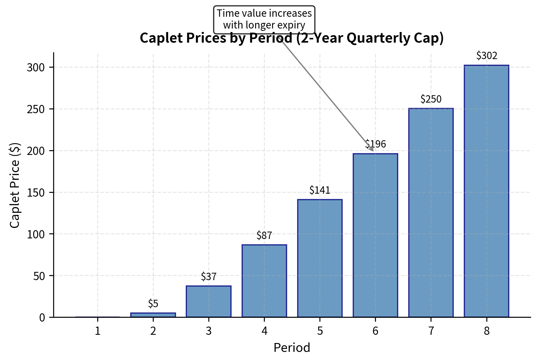
Let's price a 2-year quarterly cap with a 5% strike. We'll assume a flat yield curve at 4% for simplicity:
The first caplet has zero value because its fixing occurs at inception (time 0), and with the forward rate at 4% below the 5% strike, it's out of the money with no time for rates to move. Subsequent caplets have progressively higher values due to longer time to expiration, giving more opportunity for rates to rise above the strike. This pattern illustrates a fundamental principle of option pricing: time has value because it provides opportunity for favorable movements in the underlying.
Cap-Floor Parity
A fundamental relationship connects caps, floors, and swaps. This relationship, known as cap-floor parity, provides a consistency check for pricing.
Recall from Chapter 12 that a payer swap involves paying fixed and receiving floating. If we decompose this:
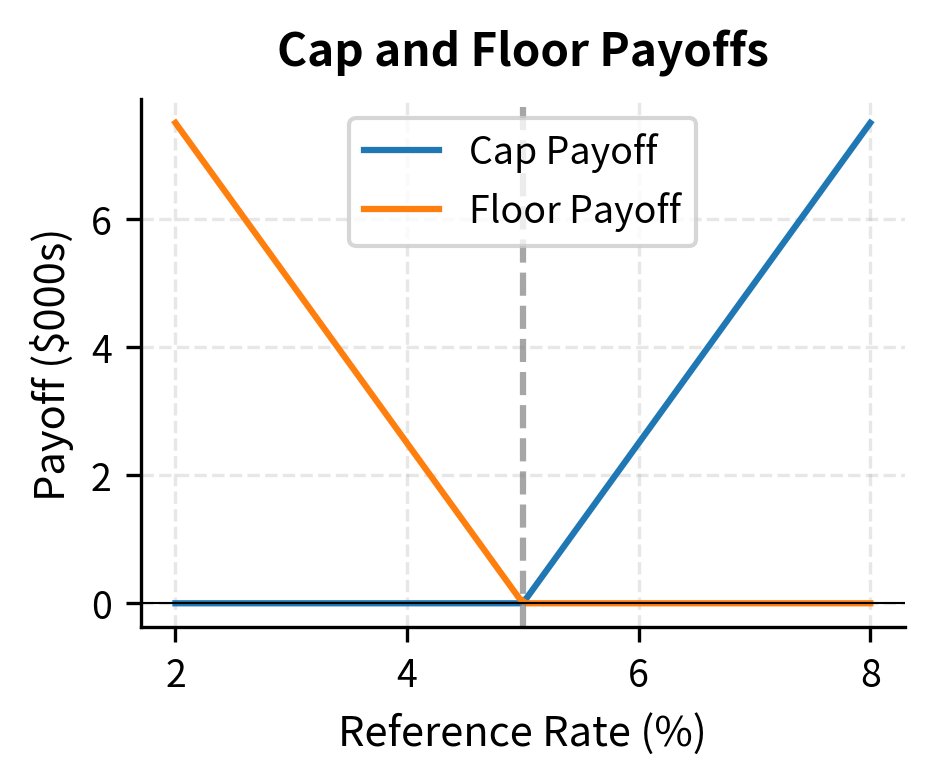
- Buying a cap with strike gives us the positive part of
- Selling a floor with strike gives us the negative part of
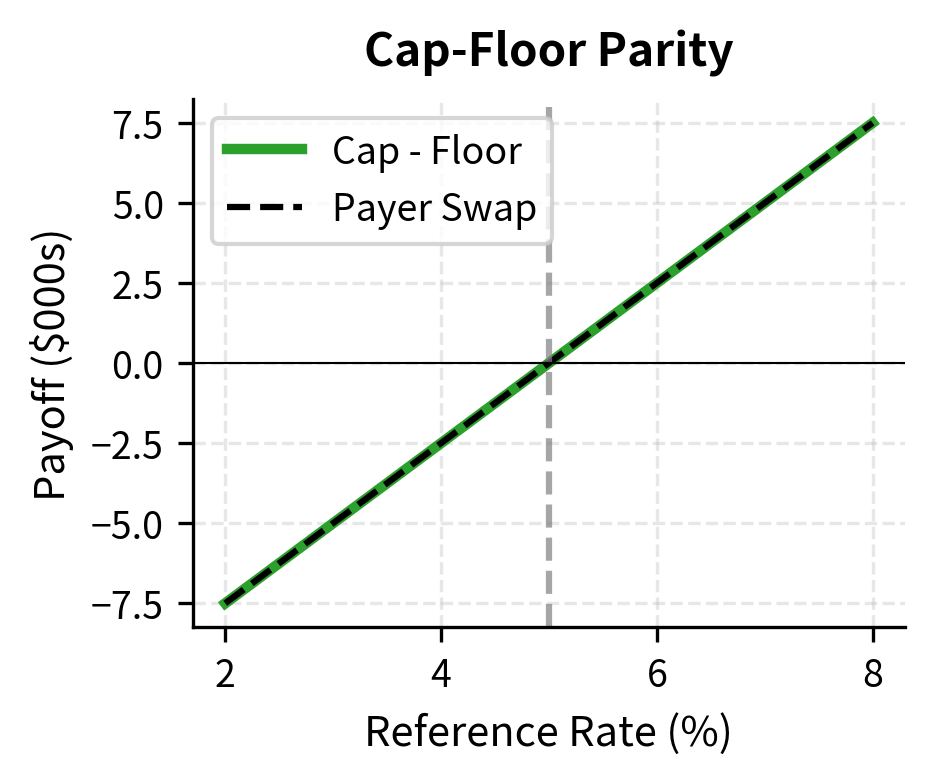
The combination yields exactly for each period. To see why this works, consider what happens in each possible state of the world. When the floating rate exceeds the strike, the cap pays us the difference while the floor expires worthless. When the floating rate falls below the strike, the cap expires worthless but we owe the floor buyer the difference. In either case, our net position equals the floating rate minus the strike.
We can see this mathematically by decomposing the payoff across the two possible states for the reference rate :
where:
- : reference interest rate observed at time
- : strike rate
Regardless of rate movements, a long cap and short floor deliver the floating rate minus the strike. This is precisely the payoff of receiving floating and paying fixed in a swap.
The right-hand side represents the floating minus fixed cashflow of a payer swap. Summing these values gives us cap-floor parity:
where:
- : price of the cap with strike
- : price of the floor with strike
- : value of a payer swap with fixed rate
When equals the current swap rate, the payer swap has zero value (it's at-the-money), so the cap and floor have equal prices. This at-the-money volatility is often the benchmark for quoting interest rate option prices. The relationship also provides a powerful arbitrage constraint: if cap and floor prices diverge from parity, you can profit by buying the underpriced combination and selling the overpriced one.
Swaptions
A swaption is an option to enter into an interest rate swap. While caps and floors provide protection against rate movements, swaptions give you a single decision point: at option expiry, you may enter a swap at pre-agreed terms or walk away. This structure is particularly useful when the decision about interest rate exposure needs to be made at a specific future date.
Swaptions come in two varieties:
- Payer swaption: The right to enter a payer swap (pay fixed, receive floating)
- Receiver swaption: The right to enter a receiver swap (receive fixed, pay floating)
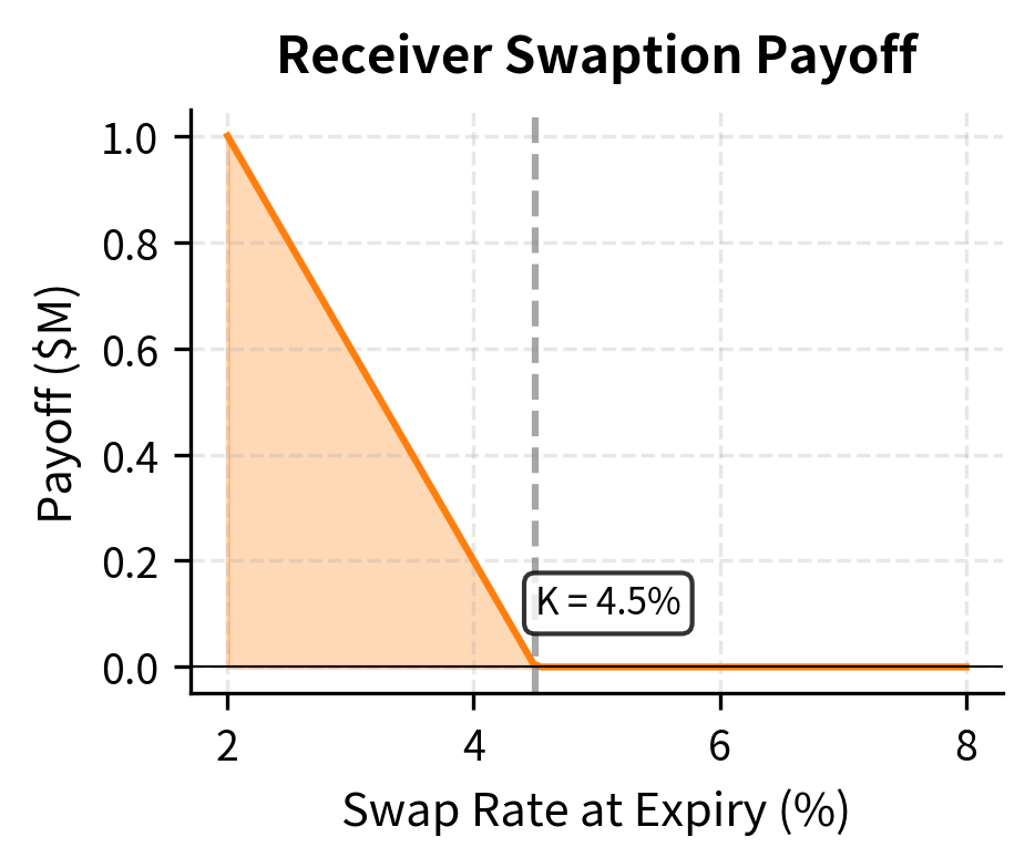
A payer swaption becomes valuable when rates rise: you can lock in paying a below-market fixed rate while receiving market floating rates. Conversely, a receiver swaption becomes valuable when rates fall: you can lock in receiving an above-market fixed rate.
Swaptions are typically quoted by their option maturity and the tenor of the underlying swap. A "2y5y payer swaption" gives you the right, in 2 years, to enter a 5-year payer swap at a predetermined fixed rate. The first number indicates how long you must wait before making the exercise decision, while the second indicates the duration of the swap that begins upon exercise.
Swaption Payoff Structure
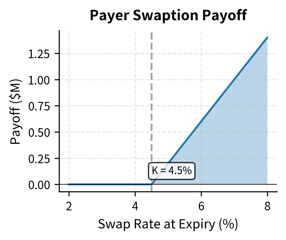
To understand swaption payoffs, consider what happens at the option's expiration date. You must decide whether to exercise, which means entering the underlying swap at the pre-agreed strike rate. This decision depends on comparing the strike rate to the prevailing market swap rate.
At expiration, you will exercise if the prevailing swap rate exceeds the strike rate. The swap you enter will have positive value because you'll pay below-market fixed rates while receiving market floating rates. The payoff equals the present value of the swap you receive. If the market swap rate is below the strike, exercise would mean paying an above-market rate, so you let the option expire worthless.
For a payer swaption with strike expiring at time , if the swap rate at expiration is :
where:
- : annuity factor at time
- : swap rate at time
- : strike rate
The structure of this payoff resembles a call option on the swap rate, with the annuity factor serving as a conversion mechanism between rates and dollars.
is the annuity factor, representing the present value at time of receiving a unit rate payment (100%) on each swap payment date (note that PVBP is typically this value scaled by 0.0001):
where:
- : number of payment periods in the swap
- : day count fraction for the -th period
- : discount factor from time to payment date
The annuity factor converts rate differences into dollar values, accounting for the timing and discounting of all swap payments. To understand why this conversion is necessary, recall that a swap rate difference of 1% does not immediately translate to 1% of notional in value. Instead, that 1% rate differential must be applied to each payment period, adjusted by the day count fraction, and then discounted back to the exercise date. The annuity factor captures all of these adjustments in a single number.
Black's Model for Swaptions
Having established the payoff structure, we now turn to valuation. We price swaptions by treating the forward swap rate as the underlying asset and applying Black's formula.
Under Black's model, the swap rate is assumed to follow a lognormal distribution under the annuity measure. This measure represents market risk-neutral expectations using the annuity stream as the unit of account. Under this measure, the forward swap rate is a martingale, meaning its expected future value equals its current value. This gives pricing formulas analogous to those for caps:
The price of a payer swaption with strike , option expiry , and notional is:
where:
- : notional principal
- : cumulative standard normal distribution function
- : current annuity factor
- : current forward swap rate
- : strike rate
- : time to option expiration
- : swaption volatility
- : measures how many standard deviations the forward swap rate is above the strike, adjusted for time and volatility
- : a risk-adjusted measure accounting for volatility over the option's life
- : expected value of the swap rate, conditional on exercise
- : strike rate weighted by the probability of exercise
For a receiver swaption:
where:
- : notional principal
- : current annuity factor
- : strike rate
- : current forward swap rate
- : swaption volatility
- : cumulative normal distribution values for the receiver swaption payoff
The swaption formula is intentionally similar to the caplet formula. In both cases, we have an option on an interest rate, discounted appropriately and multiplied by a factor that converts rates to dollars. For caplets, that factor combines the notional, day count fraction, and discount factor. For swaptions, it combines the notional and annuity factor. The annuity factor plays the role of discounting because the swaption payoff is effectively denominated in units of the annuity stream.
The volatility parameter in the swaption formula represents the implied volatility of the forward swap rate over the option's life. Unlike caplet volatilities, which vary by fixing date, swaption volatilities vary by both option expiry and underlying swap tenor. A 1-year option into a 5-year swap may have different volatility than a 2-year option into a 10-year swap, reflecting the market's assessment of uncertainty for different rate instruments.
Let's price a 1-year option into a 5-year swap:
Notice that the payer swaption is out of the money (forward rate 4% < strike 4.5%), so it's worth less than the receiver swaption. The difference equals the value of a forward-starting payer swap at the strike rate, verifying put-call parity for swaptions:
where:
- : present value of the underlying forward swap
This parity relationship mirrors cap-floor parity and serves the same purposes: it provides consistency checks for pricing and creates arbitrage bounds that keep markets aligned.
Settlement Types
Swaptions can settle in two ways:
- Physical settlement: You enter the actual swap upon exercise
- Cash settlement: You receive a cash payment equal to the swap's value
Cash-settled swaptions require agreement on how to value the swap at exercise. A common convention uses an ISDA-standard discounting method based on mid-market swap rates. The choice of settlement type can matter during market stress, when differences between cash settlement formulas and actual swap values may emerge.
Bermudan and American Swaptions
While European swaptions (exercisable only at expiry) are most liquid, Bermudan swaptions allow exercise on multiple specified dates, typically coinciding with swap payment dates. A Bermudan swaption exercisable into a 10-year swap might allow exercise at years 1, 2, 3, or 4, with the underlying swap maturing at year 11 regardless of exercise date.
The Bermudan feature adds significant complexity to valuation. At each potential exercise date, you must compare the immediate exercise value to the value of waiting and potentially exercising later. This comparison requires knowing the continuation value, which depends on what might happen in all future scenarios. The problem becomes path-dependent: the optimal exercise decision today depends on the entire history of rate movements that led to the current state.
Bermudan swaptions cannot be priced with Black's model because early exercise introduces path-dependency. They require more sophisticated techniques such as:
- Lattice methods: Building interest rate trees as discussed in Chapter 14, with backward induction to determine optimal exercise
- Monte Carlo with regression: Using least-squares Monte Carlo (Longstaff-Schwartz) to approximate the continuation value
We'll see calibration techniques for these models in the upcoming Chapter 21 on calibration and parameter estimation.
Pricing with Interest Rate Models
Black's model provides a convenient closed-form solution but assumes constant volatility and a specific distributional form. More sophisticated pricing uses the interest rate models from Chapters 14 and 15. These models capture richer dynamics, including mean reversion, time-varying volatility, and correlations between different points on the yield curve.
Short-Rate Models
The Hull-White model from Chapter 14 allows pricing via lattice methods. The key advantage of this approach is consistency: a single model, calibrated to match market prices of liquid instruments, can then price a wide variety of derivatives. This consistency becomes crucial when hedging complex positions, where we need all instruments to be valued in a coherent framework.
We build a trinomial tree for the short rate, then use backward induction to value the derivative. This approach handles path-dependent features like Bermudan exercise and provides consistent pricing across instruments. The tree structure naturally accommodates the mean reversion that characterizes interest rate dynamics, pulling rates back toward a long-run level even as random shocks push them away.
For a caplet in a Hull-White tree, the valuation proceeds in three stages. First, we build the short-rate tree out to the caplet's payment date, constructing all possible rate scenarios at each time step. Second, at the payment date nodes, we calculate the caplet payoff based on the realized rate at each scenario. Third, we work backward through the tree, discounting expected values at each node, until we arrive at today's value.
LIBOR Market Model
The LIBOR Market Model (LMM) from Chapter 15 directly models the forward rates that appear in cap and floor payoffs. This makes it particularly natural for pricing caps, as the forward rate dynamics are specified directly rather than derived from short-rate dynamics. Rather than modeling an abstract short rate and then computing forward rates, the LMM starts with the observable quantities that appear in derivative payoffs.
In the LMM, each forward rate evolves under its natural forward measure:
where:
- : forward rate for period at time
- : instantaneous volatility of the forward rate
- : Brownian motion increment under the forward measure
This equation describes how forward rates evolve randomly over time. The key feature is that under the forward measure, the drift term vanishes, leaving only the volatility-driven random component. This property, a consequence of careful measure selection, greatly simplifies pricing.
For caplet pricing, this reduces exactly to Black's model when volatility is constant. The LMM's power emerges when pricing instruments that depend on multiple forward rates, where the model captures correlations between different tenor rates. A spread option, which pays based on the difference between two rates, requires modeling how those rates move together. The LMM provides a framework for specifying and calibrating these correlations consistently.
Risk Measures for Interest Rate Derivatives
Managing a portfolio of interest rate derivatives requires understanding their sensitivities to various market factors. The primary risk measures extend the Greeks framework from Chapter 7 to the interest rate context. While the conceptual foundation remains the same, namely measuring how derivative values change with underlying factors, the specific risk factors differ when the underlying is an interest rate rather than a stock price.
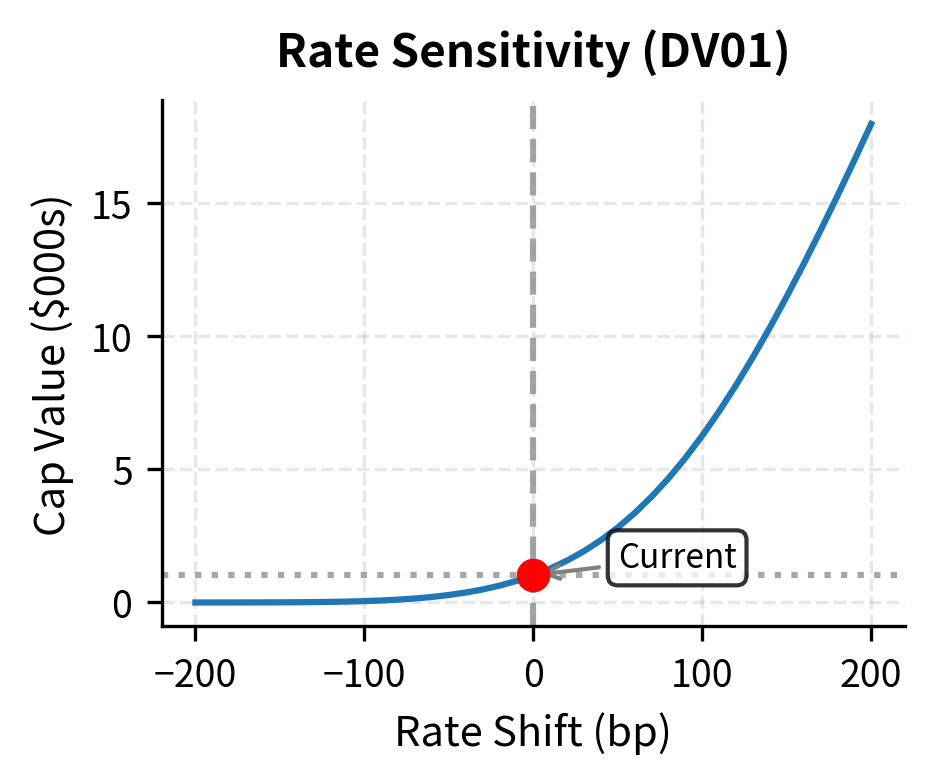
PV01 and DV01
PV01 (Present Value of a Basis Point) and DV01 (Dollar Value of a Basis Point) measure how much the derivative's value changes for a 1 basis point (0.01%) parallel shift in interest rates. These measures quantify first-order interest rate exposure and are essential for risk management.
where:
- : Dollar Value of a Basis Point
- : value of the derivative
- : level of interest rates (parallel shift)
The interpretation is straightforward: if DV01 equals $5,000 then a 1 basis point rise in rates changes the derivative's value by approximately $5,000. This measure allows you to compare and aggregate positions across different instruments, expressing everything in terms of standardized rate sensitivity.
For caps and floors, PV01 depends on the relationship between the strike and current rates. An out-of-the-money cap has lower PV01 than an at-the-money cap because rate changes have less impact on an option that's far from being exercised. As a cap moves deeper into the money, its PV01 approaches that of the underlying floating-rate exposure, reflecting the fact that deep in-the-money options behave increasingly like the underlying.
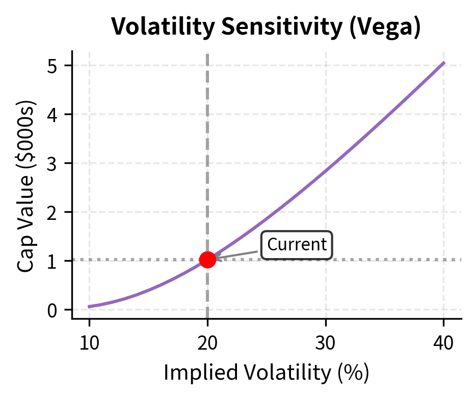
Vega and Volatility Risk
Interest rate derivatives are highly sensitive to implied volatility. Vega measures the sensitivity to a 1% absolute change in volatility. This sensitivity matters because implied volatilities change constantly in response to market sentiment, central bank communications, and economic data releases.
where:
- : sensitivity to volatility
- : value of the derivative
- : implied volatility parameter
For caps, vega is highest when the cap is at-the-money and decreases as the cap moves further in or out of the money. This pattern reflects how volatility matters most when the outcome is uncertain. A deep out-of-the-money cap will likely expire worthless regardless of volatility, while a deep in-the-money cap will almost certainly pay off. The at-the-money cap sits precisely at the boundary where volatility can tip the outcome either way.
Delta and Gamma
Delta measures sensitivity to the underlying forward rates, while gamma captures the second-order sensitivity. These measures show how the derivative's value responds to rate movements.
where:
- : first-order sensitivity to the forward rate (delta)
- : second-order sensitivity to the forward rate (gamma)
- : value of the derivative
- : underlying forward rate
Delta indicates the hedge ratio: how much of the underlying forward rate agreement we need to offset the option's rate exposure. Gamma measures convexity, indicating how quickly the delta changes as rates move. High gamma positions require frequent rebalancing, as the hedge ratio shifts with each rate movement.
For individual caplets, Black's model provides closed-form delta:
where:
- : delta of a single caplet
- : notional principal
- : day count fraction
- : discount factor to the payment date
- : the hedge ratio, representing the sensitivity of the option value to changes in the forward rate
While represents the probability of the option expiring in-the-money under the forward measure, determines the amount of the underlying required to hedge the option's risk. The distinction between these two probabilities reflects the asymmetric nature of option payoffs: we need to consider not just whether the option pays off, but how much it pays conditional on exercise.
Worked Example: Hedging Floating-Rate Exposure
Consider managing \$100 million of floating-rate debt linked to 3-month rates, resetting quarterly for the next 3 years. Current rates are 5%, and you want protection if rates exceed 6%.
Step 1: Define the Hedging Instrument
We need a 3-year quarterly cap with a 6% strike. This provides 12 caplets, one for each quarterly reset.
Step 2: Analyze Cost-Benefit
The cap costs approximately 0.16% of notional upfront. To evaluate whether this is worthwhile, consider the breakeven analysis:
The analysis shows that if rates rise to 8% or higher, the cap provides substantial protection, more than covering its initial cost.
The Volatility Surface for Interest Rate Options
Just as equity options exhibit volatility smiles and surfaces, interest rate options display complex volatility patterns across both strike and expiry dimensions.
Cap Volatility Structure
Cap volatilities are typically quoted across a matrix of strikes and expiries. The at-the-money forward (ATMF) strike corresponds to the current forward swap rate for each cap tenor. Volatilities are then quoted at various strike offsets from ATMF.
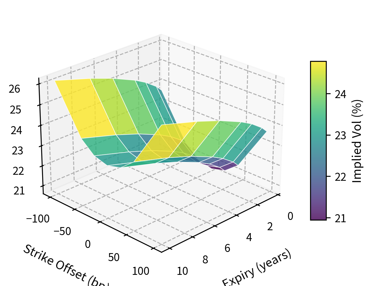
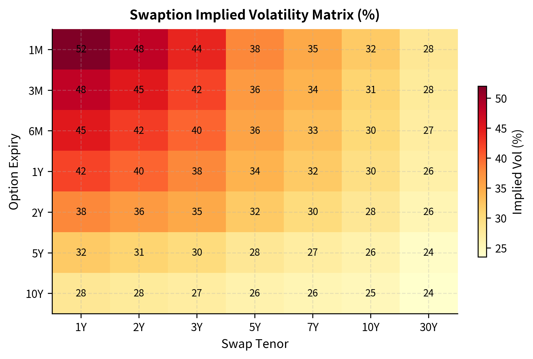
Swaption Volatility Cube
Swaption volatilities form a three-dimensional structure, varying by option expiry, underlying swap tenor, and strike. This volatility cube is fundamental to pricing and risk management in the rates market.
Market makers quote swaption volatilities in matrices such as:
| Expiry \ Tenor | 2Y | 5Y | 10Y |
|---|---|---|---|
| 1M | 45.2% | 38.1% | 32.5% |
| 6M | 42.8% | 36.5% | 31.2% |
| 1Y | 40.5% | 35.2% | 30.1% |
| 5Y | 32.1% | 28.9% | 26.5% |
The pattern typically shows higher volatilities for shorter-expiry options and shorter-tenor underlyings. This reflects the mean-reversion tendency of interest rates: longer-horizon rates exhibit less percentage volatility because they're anchored by long-term expectations.
Option-Adjusted Analysis for Mortgages
Interest rate options appear embedded in many fixed income products. The most significant example is residential mortgages, which contain a prepayment option that borrowers can exercise when rates fall.
The Prepayment Option
A fixed-rate mortgage gives the borrower the right to prepay principal at any time. This is economically equivalent to a portfolio of:
- A fixed-rate loan to you
- A call option on the loan's value, owned by the borrower
When rates fall, borrowers refinance their mortgages, prepaying existing loans and taking out new ones at lower rates. This prepayment hurts you because you receive principal back when rates are low and must reinvest at lower yields.
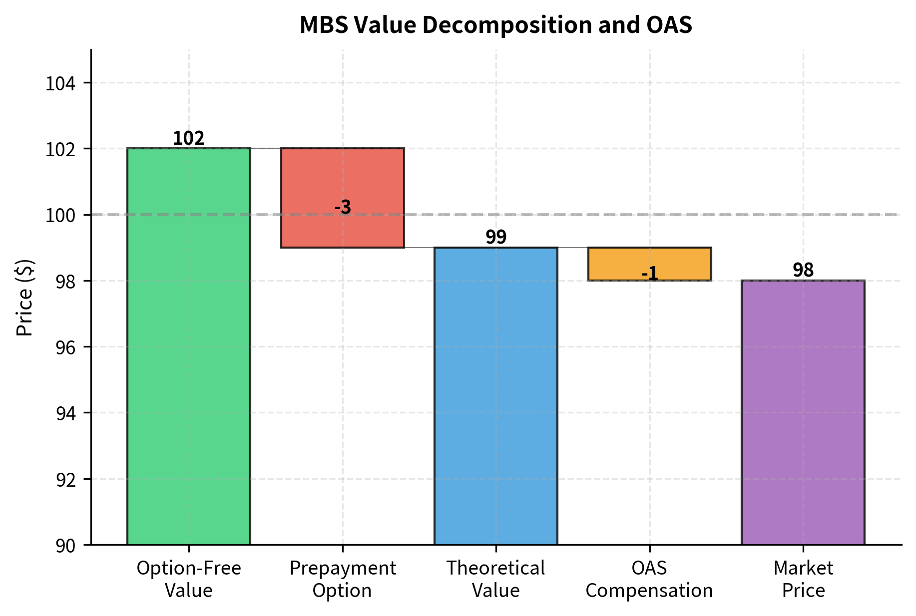
Option-Adjusted Spread
The Option-Adjusted Spread (OAS) quantifies the yield premium on mortgage-backed securities after accounting for the embedded prepayment option. The calculation involves:
- Model rate paths: Generate many interest rate scenarios using a calibrated model
- Project prepayments: Apply a prepayment model that responds to rate levels
- Calculate cashflows: Determine expected cashflows on each path
- Find the spread: Solve for the spread over the benchmark curve that makes the present value of model cashflows equal to the market price
A positive OAS indicates the security offers excess yield after adjusting for option risk. You use OAS to compare MBS against corporate bonds and other fixed income alternatives on an apples-to-apples basis.
Practical Applications and Use Cases
Interest rate derivatives serve diverse purposes across the financial industry:
Hedging Applications
- Corporate treasury: You buy caps to limit maximum interest expense
- Banks: You use floors to protect net interest margins when rates fall
- Insurance companies: You purchase swaptions to hedge guaranteed investment contracts with embedded options
- Pension funds: You use receiver swaptions to hedge against falling rates that increase liability values
Trading and Speculation
- Volatility trading: Buy caps/floors when implied volatility appears cheap relative to expected future rate volatility
- Curve trades: Use caps at different tenors to express views on curve steepening or flattening
- Event-driven: Purchase swaptions ahead of central bank meetings to position for rate surprises
Structured Product Creation
You might embed interest rate options into structured notes and deposits to create customized payoff profiles. A "capped floater" pays floating rate with a maximum coupon, funded by selling a cap to the investor.
Limitations and Practical Challenges
Black's model, while industry-standard, carries significant limitations that you must understand.
The assumption of lognormal rate distributions becomes problematic when rates approach zero or turn negative, as occurred in Europe and Japan. Lognormal models assign zero probability to negative rates, yet reality has shown otherwise. This led to the development of shifted lognormal and normal (Bachelier) models that handle negative rates appropriately. The choice of model affects both pricing and Greeks, particularly for low-strike options.
Model calibration presents ongoing challenges. Volatility surfaces evolve continuously, and models calibrated to today's market may misprice tomorrow's trades. The volatility cube contains thousands of points, each requiring consistent and stable calibration. You must balance fit quality against model stability and computational efficiency. We'll explore calibration techniques in depth in Chapter 21.
Correlation assumptions matter significantly when pricing instruments that depend on multiple forward rates. The LMM requires specifying a correlation matrix between forward rates, and different correlation structures can produce materially different prices for instruments like spread options or CMS products. Historical correlations may not persist, and there's no unique way to specify the correlation structure from market observables.
Liquidity risk poses practical challenges for hedging. While vanilla caps, floors, and swaptions trade actively in major currencies, exotic variations and longer tenors may have limited liquidity. Bid-ask spreads widen during market stress, exactly when hedging becomes most important.
Summary
Interest rate derivatives extend the option framework to the rates market, providing powerful tools for hedging and speculation on interest rate movements. The key concepts from this chapter include:
Caps and Floors are portfolios of options on interest rates. A cap protects against rising rates by paying you when the reference rate exceeds the strike. A floor protects against falling rates. Black's model provides the standard pricing framework, treating each caplet or floorlet as an option on a forward rate with lognormal dynamics.
Swaptions are options to enter interest rate swaps. Payer swaptions benefit when rates rise above the strike, while receiver swaptions benefit when rates fall. Black's model again provides the standard approach, now applied to forward swap rates. Bermudan swaptions, with multiple exercise dates, require more sophisticated lattice or simulation methods.
Risk measures for interest rate derivatives extend the Greeks framework. PV01/DV01 measures sensitivity to rate levels, while vega captures volatility exposure. Understanding these sensitivities is essential for hedging and risk management.
Practical applications span corporate hedging, bank risk management, and structured product creation. The option-adjusted spread framework helps evaluate securities with embedded optionality, such as mortgage-backed securities.
These models have limitations regarding distributional assumptions, calibration stability, and correlation. You understand both the theoretical framework and its practical boundaries.
Quiz
Ready to test your understanding? Take this quick quiz to reinforce what you've learned about interest rate derivatives valuation.

Comments