

Learn how prefix tuning adapts transformers by prepending learnable virtual tokens to attention keys and values. A parameter-efficient fine-tuning method.

This article is part of the free-to-read Language AI Handbook
Choose your expertise level to adjust how many terms are explained. Beginners see more tooltips, experts see fewer to maintain reading flow. Hover over underlined terms for instant definitions.
Prefix Tuning
While LoRA modifies how attention weights transform inputs, prefix tuning takes a fundamentally different approach: it changes what the attention mechanism sees rather than how it computes. Instead of learning low-rank updates to weight matrices, prefix tuning prepends learnable continuous vectors to the key and value sequences at each transformer layer. These virtual tokens steer the model's behavior without modifying any original parameters. This distinction is central to the method's design.
Prefix tuning is inspired by how people naturally interact with language models. Consider how discrete prompts like "Translate to French:" guide a language model toward a specific task. The presence of those words at the beginning of the input causes the model to attend to different patterns and produce different outputs than it would without them. Prefix tuning asks a natural question: what if we could learn the optimal "prompt" in continuous space, unconstrained by the vocabulary of real tokens? By removing the requirement that our steering signal map to actual words, we gain enormous flexibility. The result is a small set of task-specific vectors that guide attention without the limitations of a discrete vocabulary.
Introduced by Li and Liang in 2021, prefix tuning emerged from work on controllable generation. Prompt engineering with discrete tokens was found to be fundamentally limited by the expressiveness of individual vocabulary items. Unlike prompt engineering with discrete tokens, prefix tuning learns vectors that can represent concepts no single token could capture. These continuous vectors can encode subtle combinations of meaning, style, and task requirements that would be impossible to express through word selection alone. And unlike full fine-tuning, it leaves the pretrained model completely frozen, enabling the same base model to serve multiple tasks simply by swapping prefixes. This modularity proves particularly valuable in production environments where a single model must accommodate diverse use cases.
The Prefix Tuning Formulation
To understand prefix tuning deeply, we must first revisit how attention works and why modifying its inputs can be so powerful. The attention mechanism is the heart of the transformer architecture, responsible for determining which parts of the input sequence should influence each other. As discussed in previous chapters, scaled dot-product attention computes:
where:
- : the query matrix (what we look for)
- : the key matrix (what we match against)
- : the value matrix (what we retrieve)
- : the dimension of the key vectors
- : the function converting scores to probabilities
We scale by to prevent the dot products from growing too large, which would cause vanishing gradients in the softmax. This scaling factor ensures that regardless of the dimensionality of our key vectors, the attention scores remain in a range where the softmax function produces meaningful gradients during backpropagation.
These matrices are derived from input representations through learned linear projections. In standard transformers, these matrices come from projecting the input sequence :
where:
- : the input sequence matrix of shape
- : the learnable projection matrix mapping -dimensional input vectors to query vectors of dimension
- : the learnable projection matrix mapping -dimensional input vectors to key vectors of dimension
- : the learnable projection matrix mapping -dimensional input vectors to value vectors of dimension
This formulation reveals two potential ways to adapt model behavior. We could modify the projection matrices , , and , which is the approach taken by methods like LoRA. Alternatively, we could modify what these projections operate on by changing the sequences that become keys and values. Prefix tuning chooses the latter path.
Prefix tuning modifies the attention computation by prepending learnable prefix vectors to both keys and values. Let and be learnable prefix matrices, where is the prefix length. The modified attention becomes:
where:
- : the extended key matrix
- : the extended value matrix
- : learnable prefix matrix of shape
- : learnable prefix matrix of shape
- : original key matrix
- : original value matrix
- : concatenation operation along the sequence dimension
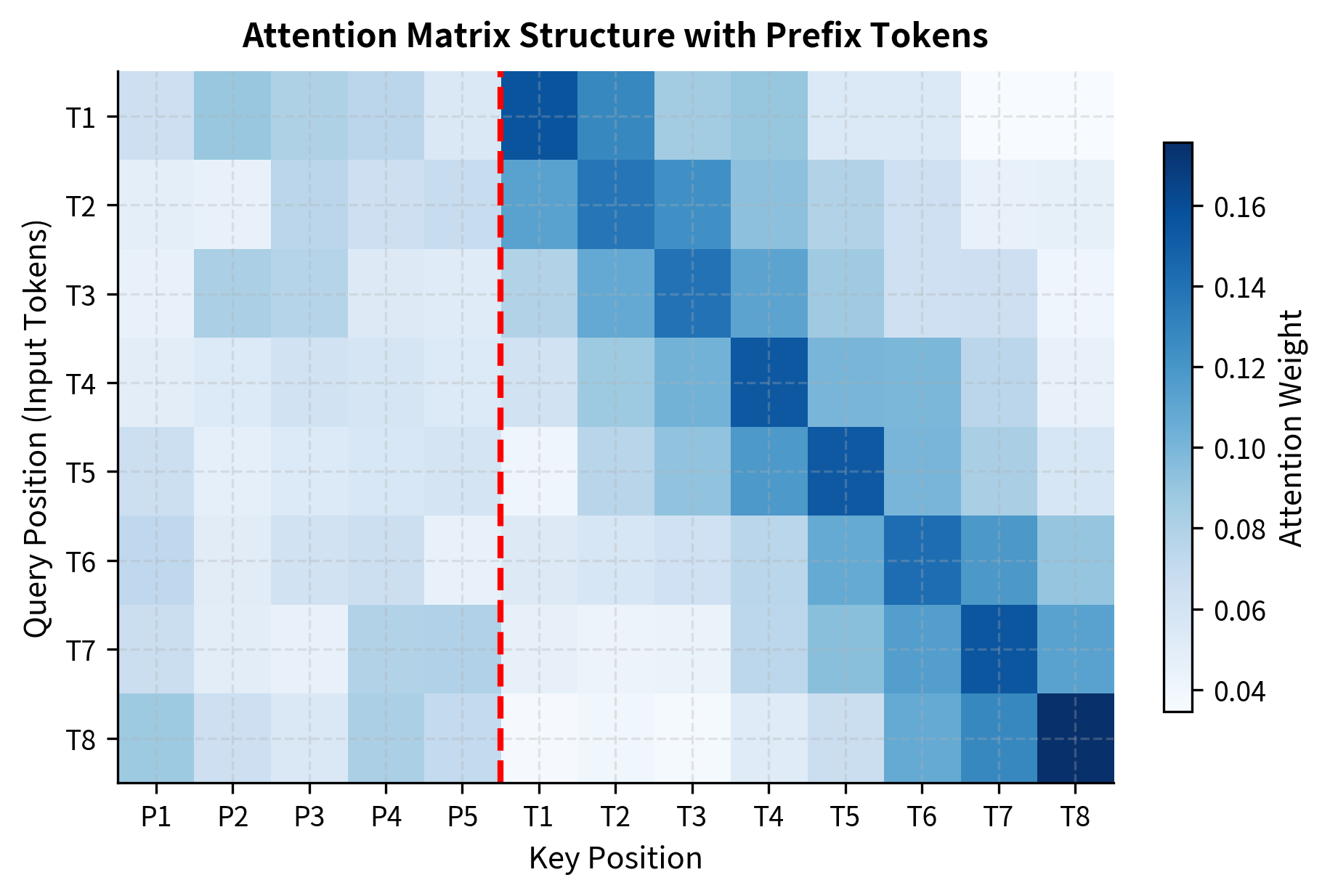
The semicolon notation indicates vertical stacking of matrices: we place the prefix matrices above the original matrices, effectively creating longer sequences. This means that when we compute attention, every query position can now attend not only to the original key positions but also to these new prefix positions. The prefix positions provide additional "options" for the attention mechanism to draw information from.
The attention computation now attends over the extended sequences:
where:
- : the query matrix (unchanged)
- : the extended key and value matrices containing prefix tokens
- : the dimension of the key vectors (scaling factor)
- : normalizes over the extended sequence length ()
Notice that the queries remain unchanged: we do not prepend anything to them. This asymmetry is intentional. The queries represent what each position in our sequence is looking for. By keeping queries tied to the actual input positions, we ensure that the output sequence maintains the same length as the input. The prefixes influence computation by providing additional things to attend to, not additional positions that produce outputs.
The prefix vectors and are called "virtual tokens" because they occupy positions in the sequence that no real input token corresponds to. Unlike token embeddings constrained to the model's vocabulary, these vectors live in continuous space and can represent arbitrary concepts. This freedom from the discrete vocabulary is what gives prefix tuning its expressive power: the learned vectors can encode task-specific information that no combination of real tokens could express as efficiently.
Layer-Specific Prefixes
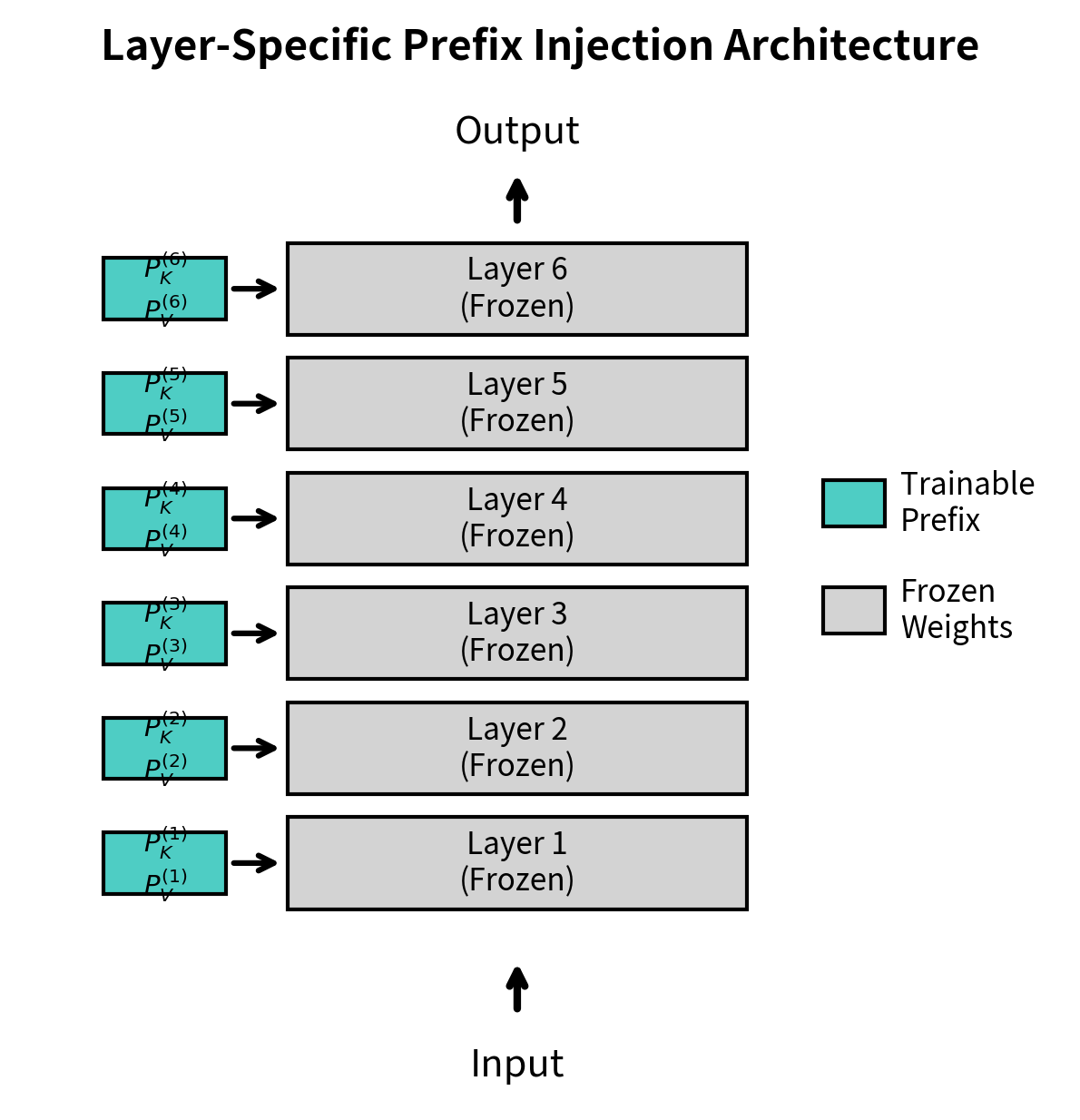
A critical detail distinguishes prefix tuning from simpler approaches: prefix tuning introduces separate prefix vectors at each transformer layer, not just at the input. This distinguishes it from methods that only modify the input embedding. For a model with layers, prefix tuning learns:
where:
- : learnable prefix matrices for the -th layer
- : total number of transformer layers
This layer-specific design is essential for achieving strong performance, and understanding why requires appreciating how transformers process information hierarchically. Each layer of a transformer captures different levels of abstraction, from syntactic patterns in early layers to semantic concepts in later ones. Early layers often detect basic linguistic features like word boundaries and simple grammatical structures. Middle layers build up more complex representations involving phrases and clauses. Later layers capture high-level semantic relationships, topic coherence, and task-relevant features. By learning prefixes at each layer, prefix tuning can guide representations at every level of the hierarchy, providing layer-appropriate steering signals that accumulate into a coherent task-specific behavior.
If we only added prefixes at the input layer, the steering signal would need to propagate through all subsequent layers, becoming diluted and potentially losing its task-specific character. By injecting fresh task guidance at every layer, prefix tuning ensures that the model receives consistent direction throughout its entire processing pipeline.
The Reparameterization Trick
Direct optimization of the prefix matrices often leads to unstable training. The loss landscape can be highly non-convex, and the prefixes can drift to regions that cause attention weights to saturate or vanish. This instability occurs because the prefix vectors interact with the attention mechanism in complex ways. Small changes to prefix values can produce large changes in attention distributions, making gradient descent erratic and prone to finding poor local minima.
To address this challenge, Li and Liang proposed a reparameterization using a small feed-forward network. The key insight is that instead of directly optimizing the high-dimensional prefix vectors, we can learn a more compact representation and project it into the required space. Instead of optimizing layer-specific prefixes directly, we learn a single smaller matrix and project it to generate prefixes for all layers:
where:
- : the learnable matrix of shape (where ), shared across layers
- : a neural network projecting to the combined dimensionality of all layer prefixes
- : an operation that divides the large MLP output into layer-specific key and value matrices
- : the resulting prefix key matrix for layer
- : the resulting prefix value matrix for layer
The MLP projects the shared to the high-dimensional space required for all layers. This architecture creates a bottleneck that constrains the space of possible prefixes, effectively regularizing the optimization. During training, we optimize and the MLP weights rather than the final prefix vectors directly. After training, we can discard the MLPs and directly use the computed and for inference, since these are fixed values that no longer need to be generated dynamically.
The MLP typically has one hidden layer with a nonlinear activation:
where:
- : the low-dimensional input vector (a row from the prefix matrix)
- : weight matrix of the first linear layer (expansion)
- : bias vector of the first linear layer
- : non-linear activation function
- : weight matrix of the second linear layer (projection to full dimension)
- : bias vector of the second linear layer
The hyperbolic tangent activation is particularly well-suited here because it bounds outputs to the range , preventing the prefix values from exploding during training. This bounded activation helps maintain numerical stability throughout the optimization process.
This reparameterization provides several important benefits:
- Training stability: The MLP constrains the prefix space, preventing extreme values that could cause attention saturation
- Better generalization: The bottleneck dimension acts as regularization, encouraging the model to learn compact, generalizable representations rather than overfitting to training data
- Smoother optimization: Gradients flow through the MLP, providing a more favorable loss landscape with fewer sharp local minima
Parameter Count
The total number of trainable parameters depends on prefix length , model dimension , number of layers , and the reparameterization dimension . Understanding this count helps us compare prefix tuning's efficiency against other methods. Without reparameterization, the total parameter count is simply the sum of all elements in the layer-specific prefix matrices:
where:
- : prefix length
- : hidden dimension
- : number of layers
- : factor for separate key and value prefixes
The factor of 2 accounts for the fact that we learn independent prefix matrices for both keys and values at each layer. Each of these matrices has rows (one per prefix position) and columns (matching the model's hidden dimension).
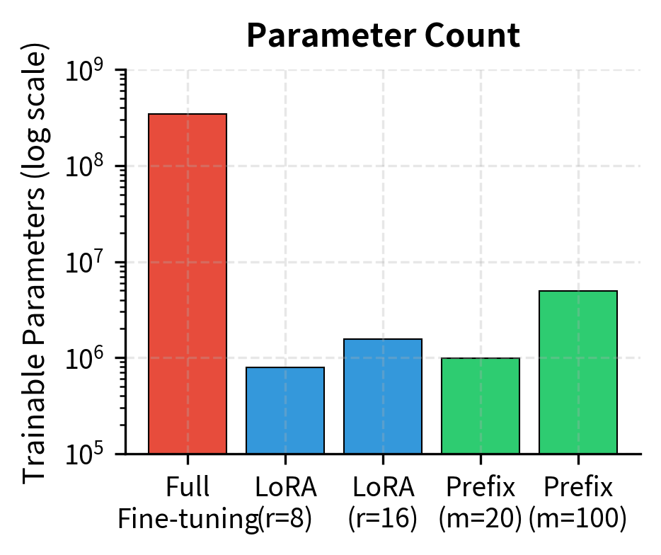
For a model like GPT-2 Medium with layers and , a prefix length of yields:
This represents roughly 0.1% of GPT-2 Medium's 345 million parameters, similar to what LoRA achieves with moderate rank settings. Learning fewer than half a million parameters can substantially alter the behavior of a model with hundreds of millions of frozen parameters. This efficiency enables practical fine-tuning even in resource-constrained environments and allows a single base model to serve many different tasks, each with its own lightweight prefix.
Prefix Length Selection
The prefix length is the primary hyperparameter controlling the capacity of prefix tuning. This single number determines how much task-specific information the prefixes can encode, making its selection crucial for achieving good performance. Too short, and the prefixes cannot capture sufficient task-specific information; the model lacks the steering capacity needed to adapt to the target behavior. Too long, and they consume attention capacity that should go to actual input tokens, while also increasing the risk of overfitting to training data rather than learning generalizable patterns.
Empirical Guidelines
Research has established several practical guidelines for selecting prefix length based on extensive experimentation across diverse tasks:
- Simple classification tasks: often suffices
- Complex generation tasks: may be necessary
- Translation and summarization: has shown strong results
- General starting point: for most tasks
The original paper found that performance improves with prefix length up to a point, then plateaus or slightly degrades as the prefixes begin to interfere with attention to actual content. For the E2E dataset (a table-to-text generation benchmark), performance increased from to , with diminishing returns beyond . This pattern, where performance rises quickly with initial prefix length increases but then flattens, appears consistently across different tasks and datasets.
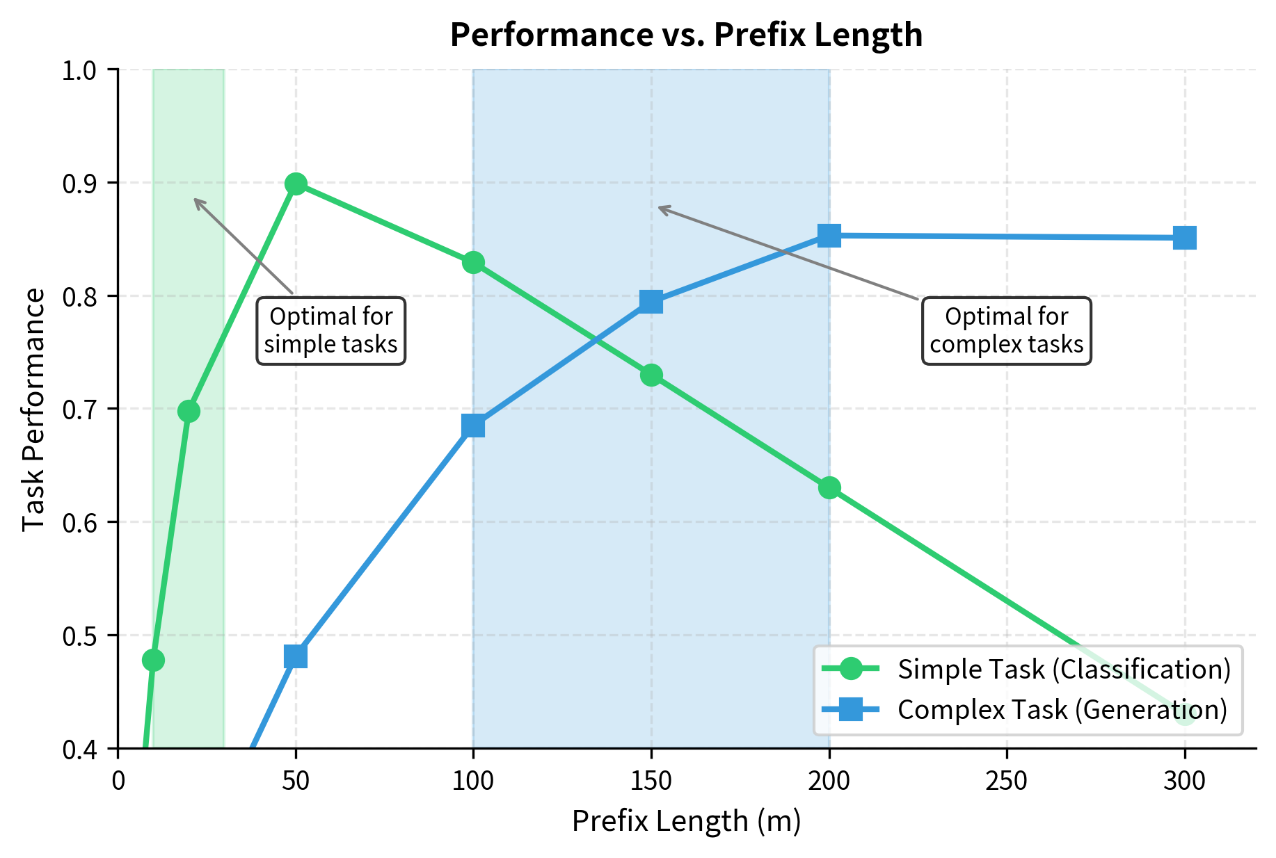
Task Complexity and Prefix Length
The relationship between task complexity and optimal prefix length follows intuitive patterns that align with how much behavioral modification the task requires:
Low-complexity tasks (sentiment classification, topic categorization) require minimal steering. The pretrained model already captures the necessary features for understanding sentiment and topics; the prefix just needs to route these existing capabilities to the appropriate output format. The adaptation is more about output formatting than deep behavioral change. Short prefixes of 10-30 tokens work well for these scenarios because the core capability already exists in the frozen model.
Medium-complexity tasks (question answering, named entity recognition) require more nuanced control. The model must learn task-specific attention patterns while leveraging pretrained knowledge, balancing what it already knows with new patterns specific to the task format. For question answering, for instance, the prefix must encode conventions about how to identify answer spans and when to abstain from answering. Prefix lengths of 50-100 tokens typically perform best for these tasks.
High-complexity tasks (open-ended generation, style transfer) require extensive behavioral modification. The prefix must encode style, format, and content preferences simultaneously, often representing subtle aesthetic choices that are difficult to express through any explicit rules. For style transfer, the prefix must capture the essence of a writing style: sentence rhythm, word choice tendencies, and structural preferences. Longer prefixes of 100-200 tokens may be necessary to encode this rich information.
Attention Budget Consideration
Each prefix token consumes attention capacity, creating a fundamental tradeoff that becomes more significant as input lengths increase. With prefix length and input length , the attention matrix grows from to . The prefixes receive attention from all input positions, potentially diluting attention to the actual content. This means that some of the "attention budget" that would normally go to understanding relationships between input tokens is instead devoted to attending to virtual tokens.
For tasks with long inputs, this tradeoff becomes significant and demands careful consideration. If your input already uses 2048 tokens and you add a prefix of 200, you're devoting roughly 9% of attention capacity to virtual tokens. For generation quality, this investment must yield proportional steering benefit. If the prefix is providing crucial task guidance that would otherwise be missing, this cost is worthwhile. However, if the task could be accomplished with a shorter prefix, the excess length only harms performance.
Start with a moderate prefix length (e.g., ) and tune based on validation performance. If performance is poor, increase the length to provide more steering capacity; if it's good but inference is slow or you're concerned about attention dilution, try reducing it to find the minimal effective length.
Prefix Tuning for Generation
Prefix tuning was originally designed for text generation tasks, where its strengths become most apparent. Unlike classification, generation requires the model to produce coherent, task-appropriate output token by token over potentially long sequences. Each generated token must be consistent with the task requirements, maintaining coherence in style, format, and content throughout. The prefix serves as persistent context that guides every generation step, providing a constant reference point that keeps the generation on track.
Autoregressive Generation with Prefixes
In autoregressive models like GPT, the prefix appears at the beginning of every forward pass and persists throughout the entire generation process. Consider generating text given an input . The generation proceeds through several stages:
- Concatenate prefix key/value matrices with input representations at each layer, establishing the initial context
- Generate the first output token attending to both prefix and input, with the prefix providing task-specific guidance
- For subsequent tokens, the prefix remains fixed while the cache of generated tokens grows, ensuring consistent steering
- Each new token can attend to the prefix, input, and all previously generated tokens, maintaining coherence with both task requirements and generated content
The prefix acts as a form of "soft system prompt" that persists throughout generation. Unlike discrete prompts that consume input context window space, prefix vectors exist in a separate namespace, only appearing in the key-value pairs. This separation is significant: the prefix does not compete with input tokens for positions in the context window, allowing the full context capacity to be devoted to actual content while still receiving task guidance.
Controlling Generation Style
Prefix tuning excels at controlling generation style because it can encode nuanced preferences that no discrete token could capture. The continuous nature of the prefix vectors allows them to represent subtle combinations of characteristics: the formality level, sentence complexity, vocabulary preferences, and structural patterns that together define a writing style. Consider training prefixes for different styles:
- Formal prefix: Learned on academic writing, technical documentation
- Casual prefix: Learned on conversational text, social media
- Creative prefix: Learned on fiction, poetry
At inference time, swapping prefixes instantly switches the model's generation style without any parameter changes to the base model. The same frozen GPT model can produce academic prose with one prefix and casual conversation with another. This modularity makes prefix tuning attractive for multi-tenant systems where you need different behaviors from the same underlying model. A single deployment can serve diverse needs simply by selecting the appropriate prefix.
Table-to-Text Generation
Prefix tuning works well for table-to-text generation. This task requires the model to follow formatting conventions while producing natural language. Consider a table:
| Name | Area | Food | Rating |
|---|---|---|---|
| The Eagle | riverside | Japanese | 5 out of 5 |
The task is to generate: "The Eagle is a Japanese restaurant near the riverside with a perfect rating."
Prefix tuning captures the conventions of this transformation: how to order attributes, which phrasing patterns to use, and how to express ratings. The prefix encodes these conventions implicitly, guiding generation without explicit templates. The model learns that names typically come first, that locations are introduced with "near" or "in," and that ratings should be expressed naturally rather than numerically. These patterns emerge from training on examples, encoded in the continuous prefix vectors in ways that would be difficult to specify through rules.
Prefix Tuning vs LoRA
Prefix tuning and LoRA use different principles. Understanding these differences helps you choose the right method for your task.
Where They Apply Changes
LoRA modifies the weight matrices themselves. As we covered in the LoRA chapters, it adds low-rank updates to the query, key, value, and output projection matrices:
where:
- : the adapted effective weight matrix
- : the frozen pretrained weights
- : the low-rank update matrix
- : low-rank decomposition matrix
- : low-rank decomposition matrix
The model computes the same operations as before, but with slightly different weights. Every forward pass through a LoRA-adapted layer produces different intermediate representations because the linear transformations themselves have changed. This means that LoRA directly modifies how the model represents information.
Prefix tuning modifies the inputs to attention rather than the weights. The projection matrices remain unchanged, but attention sees additional virtual tokens:
where:
- : the key input to the attention mechanism
- : the value input to the attention mechanism
- : the learnable prefix key matrix
- : the learnable prefix value matrix
- : the standard key projection of the input text
- : the standard value projection of the input text
- : concatenation of virtual and real tokens
The weights are identical to the pretrained model; only the data flowing through attention changes. The model applies the same transformations as before, but to an expanded set of inputs. This distinction is subtle but important: LoRA changes the function being computed, while prefix tuning changes the inputs to an unchanged function.
Expressivity and Task Fit
This architectural difference leads to different strengths that make each method better suited to particular task categories:
LoRA excels at:
- Tasks requiring fine-grained representation changes
- Classification where features need adjustment
- Situations where input structure varies significantly
- Tasks where "what the model knows" needs updating
Prefix tuning excels at:
- Generation tasks requiring consistent style/format
- Tasks with fixed output conventions
- Multi-task scenarios with prefix switching
- Situations where input structure is consistent
Empirically, LoRA often performs better on discriminative tasks (classification, NER), while prefix tuning performs competitively on generative tasks (summarization, translation). However, both methods have improved substantially since their introduction through better hyperparameter choices and training procedures, and the gap has narrowed considerably.
Computational Considerations
The methods also differ in computational cost, which affects both training and deployment decisions:
| Aspect | LoRA | Prefix Tuning |
|---|---|---|
| Training FLOPs | Slightly higher (extra matmul) | Standard attention cost |
| Inference FLOPs | Same as training | Same as training |
| Memory (activations) | Similar to base | Higher (extended sequences) |
| Memory (parameters) | Depends on rank | Depends on prefix length |
| Merging possible | Yes (into base weights) | No (separate prefix needed) |
A key distinction: LoRA adapters can be merged into the base model weights for deployment, eliminating any inference overhead. Prefix tuning requires maintaining separate prefix vectors that must be prepended at every forward pass. For serving scenarios with strict latency requirements, this overhead, though small, may be unacceptable.
Combining Methods
Prefix tuning and LoRA are not mutually exclusive. Recent work has explored combining them to capture the benefits of both approaches:
- Use prefix tuning for high-level task steering
- Use LoRA for fine-grained representation adjustment
- Achieve the benefits of both with modest parameter increase
This combination can be particularly effective for complex tasks requiring both stylistic control (prefix) and knowledge adaptation (LoRA). The prefix handles "how to respond" while LoRA handles "what to know."
Code Implementation
Let's implement prefix tuning for a GPT-2 model. We'll build the components step by step, showing how prefix vectors integrate with transformer attention.
Defining the Prefix Module
The core of prefix tuning is a module that generates layer-specific key and value prefixes. We'll implement the reparameterization trick for stable training.
The prefix encoder generates key-value pairs for each layer. The shape reflects the structure: for each sample in the batch, we have prefixes for each layer, split into key and value components, organized by attention head.
Computing Parameter Counts
Let's verify the parameter efficiency of prefix tuning.
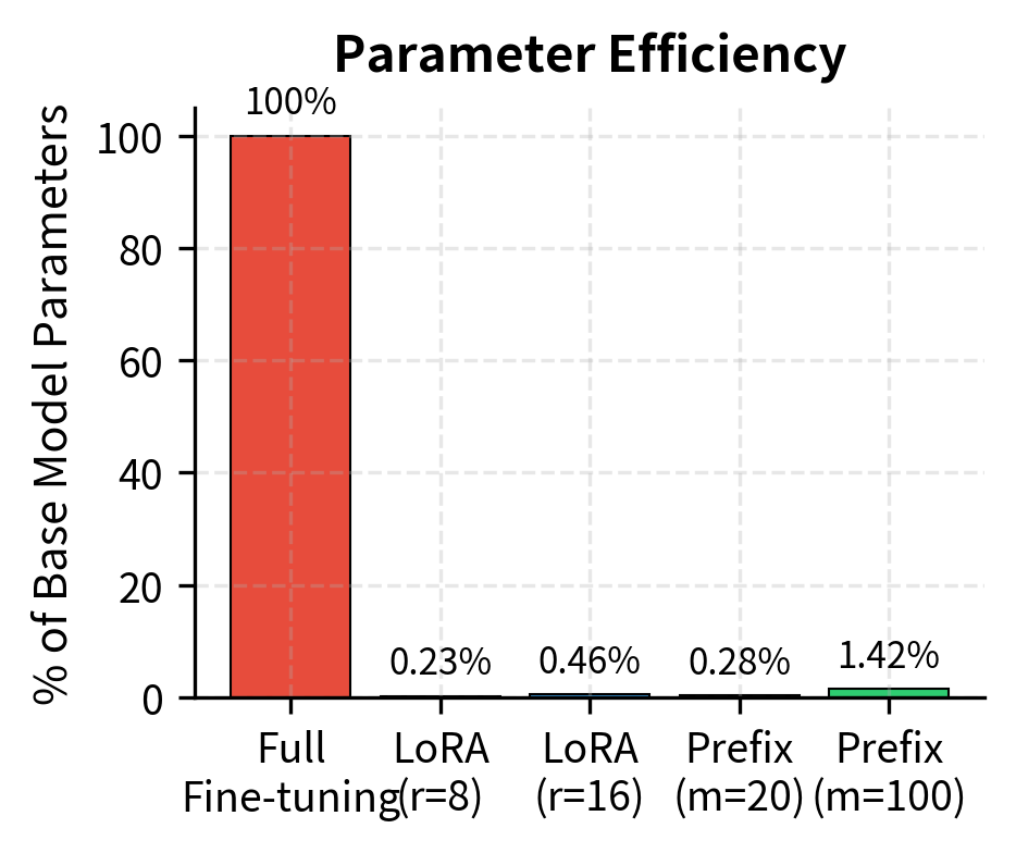
The model contains the same total parameters as the base GPT-2, but only the prefix encoder parameters (approx. 0.1%) are trainable. This drastic reduction in trainable weights demonstrates the parameter efficiency of the method.
Training Loop Example
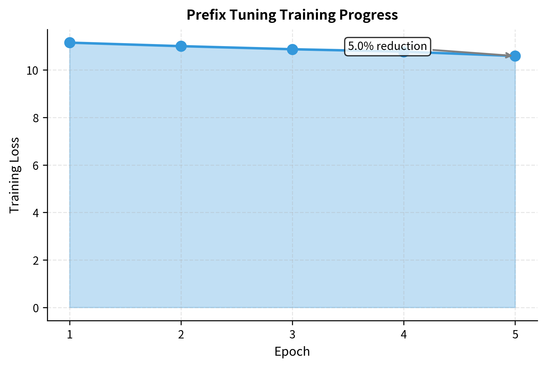
Let's demonstrate a simplified training loop for prefix tuning.
The decreasing loss indicates that the model is successfully optimizing the prefix vectors to minimize prediction error. Even with the base model frozen, the prefixes provide enough steering capacity to adapt the model's output distribution.
Visualizing Prefix Effects
Let's visualize how the learned prefix affects attention patterns.
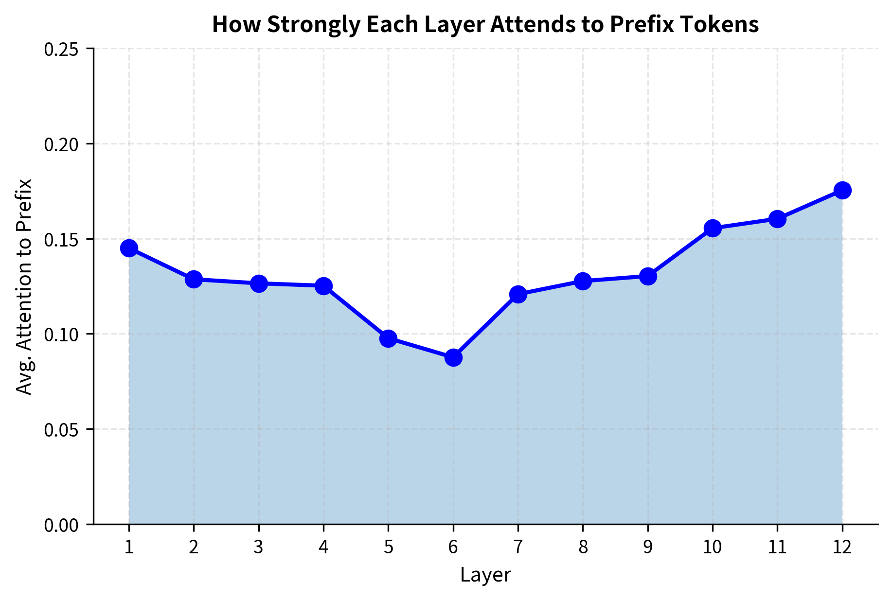
The attention pattern reveals how prefix tuning influences different layers. Typically, early layers use the prefix to establish basic task context, while later layers may reference it for output-specific guidance.
Comparing Prefix Lengths
Let's compare how different prefix lengths affect parameter count and capacity.
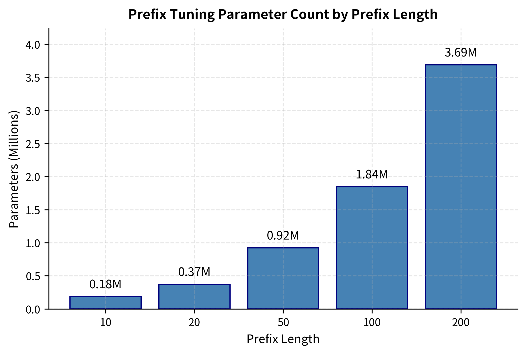
The parameter count grows linearly with prefix length. For most tasks, prefix lengths of 20-100 provide a good balance between expressivity and efficiency.
Key Parameters
The key parameters for Prefix Tuning are:
- prefix_length: The number of virtual tokens added to the sequence. Longer prefixes increase capacity but consume attention budget.
- prefix_hidden_dim: The dimension of the reparameterization MLP. A larger dimension allows for more complex mappings during training.
- num_epochs: Number of training passes. Since we are training fewer parameters, convergence can sometimes be faster than full fine-tuning.
- learning_rate: The step size for the optimizer, applied only to the prefix encoder parameters.
Limitations and Practical Considerations
Prefix tuning offers compelling advantages for parameter-efficient fine-tuning, but several limitations affect its practical applicability. Understanding these helps you decide when prefix tuning is the right choice for your task.
The most significant limitation is the attention budget consumed by prefix tokens. Unlike LoRA, which modifies weights without changing sequence length, prefix tuning extends every attention computation. For models with long context windows processing near-capacity inputs, the additional prefix positions compete with input tokens for attention resources. In extreme cases with very long prefixes (e.g., 200+ tokens) and long inputs, this competition can degrade performance on the actual task. The model may spend attention capacity on virtual tokens that would be better allocated to understanding the real input.
Training stability presents another challenge, which motivated the reparameterization trick. Without the MLP bottleneck, prefix vectors can drift to extreme values during optimization, causing attention weights to saturate. While reparameterization helps, it adds complexity: you must tune both the prefix length and the MLP hidden dimension. The MLP also adds parameters and computation during training, though it can be eliminated after training by computing the final prefix values directly.
Prefix tuning also struggles with tasks requiring input-dependent adaptation. The prefix is the same for every input in a batch, providing consistent global guidance but no input-specific modulation. If your task requires different behaviors for different inputs (e.g., different writing styles for different audiences within the same fine-tuning run), prefix tuning may underperform methods like LoRA that modify representations directly. The next chapter on prompt tuning addresses this limitation through input-dependent soft prompts.
Finally, prefix tuning lacks the merge capability that makes LoRA attractive for deployment. LoRA adapters can be absorbed into base model weights, eliminating inference overhead. Prefix tuning requires maintaining separate prefix vectors that must be prepended at every forward pass. For serving scenarios with strict latency requirements, this overhead, though small, may be unacceptable.
Despite these limitations, prefix tuning has had lasting impact on the field. It demonstrated that modifying attention inputs could be as effective as modifying weights, opening the door to a family of soft prompt methods. The insight that continuous vectors can represent concepts beyond the discrete vocabulary influenced subsequent work on prompt tuning and controllable generation. And its parameter efficiency, achieving competitive results with less than 1% of base model parameters, helped establish that massive models need not require massive fine-tuning budgets.
Summary
Prefix tuning provides a parameter-efficient alternative to full fine-tuning by prepending learnable continuous vectors to the key and value sequences in attention. Rather than modifying model weights like LoRA, it changes what the attention mechanism sees, steering behavior through persistent virtual context.
The key concepts from this chapter are:
- Formulation: Prefix tuning concatenates learnable matrices and to the key and value sequences at each transformer layer, extending the attention scope without changing weights
- Reparameterization: Training stability improves by generating prefixes through a small MLP rather than optimizing them directly
- Prefix length: The primary hyperparameter, typically ranging from 10-200 depending on task complexity, with longer prefixes for generation tasks
- Generation focus: Prefix tuning excels at controlling generation style and format, providing consistent task guidance throughout autoregressive decoding
- Comparison with LoRA: While LoRA modifies weights and can be merged for inference, prefix tuning modifies inputs and requires maintaining separate prefix vectors
The method achieves competitive performance with a small fraction of base model parameters, making it practical for adapting large language models to specific tasks. For generation tasks requiring consistent style or format, prefix tuning offers an elegant solution that keeps the base model completely frozen while providing powerful task-specific guidance.
Quiz
Ready to test your understanding? Take this quick quiz to reinforce what you've learned about prefix tuning and its role in parameter-efficient fine-tuning.

Comments