

Learn how adapter layers insert trainable bottleneck modules into transformers for parameter-efficient fine-tuning. Covers architecture, placement, and fusion.

This article is part of the free-to-read Language AI Handbook
Choose your expertise level to adjust how many terms are explained. Beginners see more tooltips, experts see fewer to maintain reading flow. Hover over underlined terms for instant definitions.
Adapter Layers
While LoRA modifies attention weights through low-rank decomposition and prefix tuning prepends learnable tokens to the input, adapter layers take a different architectural approach: they insert small, trainable neural network modules directly into the transformer's forward pass. These compact bottleneck modules learn task-specific transformations while leaving the original model weights completely frozen.
Adapters emerged from a simple observation: if we want to add new capabilities to a pretrained model without disrupting what it already knows, why not add new components rather than modify existing ones? This additive approach provides a clean separation between pretrained knowledge and task-specific adaptations, making it possible to store multiple specialized versions of a model using only a fraction of the original parameters.
In this chapter, we'll explore the adapter architecture in detail, examining how bottleneck modules compress and expand hidden representations, where to place adapters within transformer blocks for maximum effectiveness, and how to choose the right dimensionality for your task. We'll also cover adapter fusion, a technique for combining multiple task-specific adapters to enable flexible multi-task learning.
Adapter Architecture
The core idea behind adapters is straightforward: insert small bottleneck neural networks into each transformer layer that can learn task-specific transformations. To understand why this approach works, consider what happens when you fine-tune a pretrained model on a new task. The model needs to adjust how it processes information, but most of what it learned during pretraining remains relevant. Rather than modifying the carefully tuned weights that encode this valuable knowledge, adapters provide dedicated pathways for learning new behaviors.
These modules are called "bottleneck" architectures because they first compress the hidden representation to a much smaller dimension, apply a nonlinearity, and then project back to the original dimension. This compression serves a dual purpose: it dramatically reduces the number of parameters needed for adaptation, and it acts as a regularizer that forces the adapter to capture only the most essential task-specific information.
A bottleneck architecture compresses data through a narrow intermediate representation before expanding it back. This forces the network to learn a compact encoding of the relevant information, acting as an information bottleneck. The concept draws from information theory, where limiting the bandwidth of a channel forces the sender to prioritize the most important signals. In the context of neural networks, this compression encourages the adapter to identify and preserve only those features of the input that are most relevant for the downstream task.
The Adapter Module
An adapter module consists of three components arranged sequentially, each serving a specific purpose in the transformation pipeline. The architecture mirrors the structure of an autoencoder, where information is first compressed and then reconstructed, but here the goal is not reconstruction fidelity but rather learning a useful transformation of the input representation.
The three components work together as follows:
- Down-projection: A linear layer that compresses the hidden dimension to a smaller bottleneck dimension . This projection acts as a learned feature selector, identifying which aspects of the high-dimensional hidden state are most relevant for the task at hand.
- Nonlinearity: An activation function (typically ReLU or GELU) that enables nonlinear transformations. Without this component, the composition of two linear layers would simply be another linear transformation, severely limiting the adapter's expressive power.
- Up-projection: A linear layer that expands from dimension back to . This projection reconstructs the full hidden dimension, translating the compressed task-specific representation back into a form compatible with subsequent transformer layers.
Given an input hidden state , the adapter computes its output through the sequential application of these three components:
To understand this formula, let's examine each component:
- : the output of the adapter module, which represents the task-specific transformation that will be added to the original hidden state
- : the input hidden state, a vector of dimension that encodes the current representation at this point in the transformer
- : the down-projection weight matrix with shape , which compresses the input from dimension to . Each row of this matrix can be thought of as a learned detector for a particular pattern in the input
- : the bias vector for the down-projection layer, with dimension . This allows the adapter to shift the compressed representation as needed
- : the nonlinear activation function (e.g., ReLU or GELU) that enables the network to learn complex patterns. The choice of activation function affects both the expressiveness of the adapter and its training dynamics
- : the up-projection weight matrix with shape , which expands the representation back from to . This matrix translates the bottleneck representation into modifications for the full hidden space
- : the bias vector for the up-projection layer, with dimension . Often initialized to zero to ensure near-identity behavior at the start of training
Information flows through this formula from the inside out. First, the input hidden state is multiplied by the down-projection matrix and shifted by the bias, yielding a compressed representation. Next, the activation function introduces nonlinearity, allowing the adapter to model complex relationships. Finally, the up-projection expands this compressed, transformed representation back to the original dimension.
Residual Connection
A critical design choice is wrapping the adapter in a residual connection. This architectural decision fundamentally shapes how the adapter integrates with the transformer and has significant implications for both training dynamics and the nature of the learned transformation.
where:
- : the output hidden state after applying the adapter, which will be passed to subsequent operations in the transformer
- : the input hidden state from the previous layer or sublayer, preserved unchanged and added to the adapter output
- : the task-specific transformation computed by the bottleneck module, which represents the "delta" or modification to apply
This residual structure serves multiple purposes that together make adapters both effective and practical. First, it enables the adapter to learn only the delta (change) needed for the new task, rather than having to reproduce the entire transformation. This is conceptually powerful because the adapter need not learn to pass through information that should remain unchanged; instead, it can focus entirely on what needs to be different for the new task. The original representation flows through the skip connection unchanged, and the adapter simply adds whatever modifications are necessary.
Second, the residual structure allows for near-identity initialization, where adapters initialized to output near-zero values will pass through the original representations unchanged. This property is crucial for stable training because it means the model starts from a state equivalent to the pretrained model. Early in training, before the adapters have learned meaningful transformations, the model's behavior remains close to the original, avoiding the disruption that could occur if adapters initially produced large, random modifications.
Third, it provides stable gradient flow during training, as discussed in the residual connections chapter from Part XII. Gradients can flow directly through the skip connection without passing through the adapter's nonlinearity, ensuring that learning signals reach all parts of the network even when the adapter produces small outputs.
Parameter Count
Understanding the parameter count helps you appreciate adapter efficiency. For a single adapter module, the total number of trainable parameters is the sum of all weights and biases in the two projection layers:
Let's break down each term to see where the parameters come from:
- : the bottleneck dimension, typically chosen to be much smaller than the hidden dimension (e.g., 64)
- : the model's hidden dimension, determined by the base model architecture (e.g., 768 for BERT-base)
- : the number of parameters in the down-projection weight matrix, which must map from dimensions to dimensions
- : the number of parameters in the down-projection bias, one for each output dimension
- : the number of parameters in the up-projection weight matrix, which maps from back to
- : the number of parameters in the up-projection bias
- : the approximate parameter count when , showing that the two projection matrices dominate the size while the bias vectors contribute relatively little
When , this simplifies to approximately parameters per adapter, since the bias terms become negligible. For a model with hidden dimension and bottleneck dimension , each adapter contains roughly parameters, which is tiny compared to the millions of parameters in each transformer layer. To put this in perspective, a single self-attention layer in BERT-base has over 2 million parameters, so an adapter adds less than 5% overhead to each layer.
Adapter Placement
Where you insert adapters within the transformer block significantly impacts both performance and parameter efficiency. The transformer layer consists of multiple sublayers, each performing a distinct function, and the choice of where to place adapters determines which computations the adapter can influence. We have explored several placement strategies, each with different trade-offs between expressiveness, efficiency, and training stability.
Original Placement (Houlsby et al.)
The original adapter paper by Houlsby et al. (2019) proposed inserting two adapter modules per transformer layer. This comprehensive approach ensures that adapters can modify representations both after contextual mixing occurs in the attention sublayer and after feature transformation in the feed-forward sublayer. The two insertion points are:
- After the multi-head attention sublayer: Between the attention output and the first layer normalization. This position allows the adapter to modify how attended information is integrated.
- After the feed-forward network sublayer: Between the FFN output and the second layer normalization. This position enables the adapter to adjust the feature transformations applied by the FFN.
This placement follows the existing residual connection pattern established in the transformer architecture. To understand how adapters integrate with the standard transformer computation, recall that the original transformer layer computation proceeds as follows:
In these equations:
- : the intermediate representation after the attention sublayer, which captures contextually mixed information
- : the layer normalization operation that stabilizes training by normalizing activations across the feature dimension
- : the input to the transformer layer, which may come from the embedding layer or a previous transformer layer
- : the Multi-Head Attention mechanism that computes contextual relationships between tokens
- : the final output of the transformer layer, ready to pass to the next layer
- : the Feed-Forward Network sublayer that applies position-wise transformations to each token independently
With adapters inserted according to the Houlsby placement strategy, the adapted layer becomes:
Here, each component plays the following role:
- : the intermediate representation after the adapted attention sublayer, now incorporating task-specific modifications to the attention output
- : the layer normalization operation, unchanged from the original architecture
- : the input to the transformer layer
- : the first adapter module inserted after attention, which learns to modify how attention information should be adjusted for the specific task
- : the Multi-Head Attention mechanism, with frozen weights
- : the final output of the adapted transformer layer
- : the second adapter module inserted after the feed-forward network, which learns task-specific adjustments to the feature transformations
- : the Feed-Forward Network sublayer, with frozen weights
Note that the adapter is applied to the sublayer output before the residual connection with the input. This ordering is deliberate: it allows the adapter to transform the sublayer's contribution while still preserving the original skip connection's ability to pass information through unchanged.
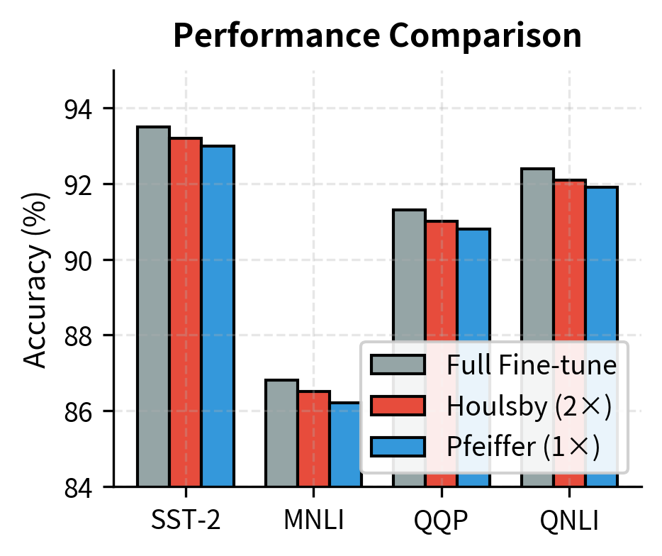
Efficient Placement (Pfeiffer et al.)
Later work by Pfeiffer et al. (2021) made a surprising discovery: using a single adapter per layer, placed only after the feed-forward network, achieves comparable performance with half the parameters. This finding challenged the assumption that both insertion points were necessary and led to more efficient adapter configurations becoming the standard practice.
The intuition behind this finding connects to what we learned about transformer components in Part XII. Feed-forward networks act as key-value memories that store factual knowledge, while attention layers handle contextual mixing. Task adaptation often requires modifying how the model processes and retrieves information, which aligns more closely with the FFN's role. When adapting a model for sentiment analysis, for example, the model primarily needs to adjust which features are emphasized and how they are transformed, rather than fundamentally changing how tokens attend to each other.
Furthermore, the attention mechanism is already quite flexible due to the query-key-value decomposition, which allows different relationships to be captured without weight modifications. The FFN, in contrast, applies fixed transformations that may need task-specific adjustment. By placing adapters after the FFN, we directly address the component most likely to need modification.
Parallel Adapters
An alternative to sequential placement is parallel adapters, where the adapter computation runs alongside the original sublayer rather than after it. This design represents a departure from the standard "intercept and modify" approach, instead treating the adapter as an independent contribution to the layer output.
In this formulation:
- : the output of the layer, combining contributions from the input, the attention mechanism, and the adapter
- : the input to the layer, which serves as the common source for all three pathways
- : the attention sublayer output, computed from the input as in the standard transformer
- : a scaling factor that controls the adapter's contribution to the final representation. This hyperparameter allows fine-grained control over how much the adapter influences the output
- : the adapter computation running in parallel with the attention mechanism, operating directly on the layer input rather than on the attention output
Parallel placement can offer computational advantages on hardware that supports concurrent operations, as the adapter and original sublayer can be computed simultaneously. On modern GPUs and TPUs, this parallelism can translate to reduced wall-clock time even though the total computation is the same. Additionally, parallel placement changes the gradient flow: the adapter receives gradients directly from the layer output without having to backpropagate through the attention computation, which can lead to different optimization dynamics.
Placement Comparison
The choice of adapter placement involves trade-offs between several competing factors:
- Parameter efficiency: Single FFN-only adapters use half the parameters of dual placement, which translates directly to storage savings when maintaining many task-specific adapters
- Performance: Dual placement often achieves slightly better results on diverse tasks, particularly when tasks require modifying both contextual mixing and feature transformation
- Training stability: The original dual placement provides more gradient pathways, potentially making optimization easier for difficult tasks
- Inference overhead: More adapters mean more sequential computations, increasing latency during inference
For most practical applications, the single adapter placement after the FFN provides an excellent balance of efficiency and performance. The savings in parameters and inference time typically outweigh the marginal performance improvements of dual placement, especially when deploying multiple adapters for different tasks.
Adapter Dimensionality
The bottleneck dimension is the primary hyperparameter controlling the trade-off between adapter capacity and parameter efficiency. Choosing the right value requires understanding how information flows through the bottleneck and how compression affects the adapter's ability to learn useful transformations.
The Information Bottleneck Perspective
When we compress a hidden representation from dimension to dimension , we're forcing the adapter to identify and preserve the most task-relevant information. This compression acts as a form of regularization, preventing the adapter from memorizing noise in the training data. The principle at work here connects to information theory: by limiting the capacity of the channel through which task information must flow, we force the adapter to be selective about what it encodes.
Consider a hidden representation compressed to dimensions. The adapter must encode whatever task-specific transformation it needs to make using only 64 degrees of freedom. This constraint encourages the adapter to learn generalizable patterns rather than fitting to idiosyncrasies in the training set. If a particular feature of the training data is not consistently useful for the task, the limited bottleneck capacity will prevent the adapter from dedicating parameters to capturing it.
The compression also has implications for what kinds of transformations adapters can represent. With a 12:1 compression ratio, the adapter cannot simply learn an arbitrary linear transformation of the input. Instead, it must identify a low-dimensional subspace that captures the essential variation needed for task adaptation. This constraint is often beneficial, as it biases the adapter toward learning transformations that align with the structure already present in the pretrained representations.
Dimensionality Guidelines
Research and practical experience suggest the following guidelines for choosing adapter dimensions, with the appropriate choice depending on task complexity, data availability, and computational constraints:
- Very small ( to ): Suitable for tasks closely related to pretraining or when data is extremely limited. Provides strong regularization but limited expressiveness. These minimal adapters work best when the task primarily requires recombining existing features rather than learning fundamentally new representations.
- Small ( to ): A good default for most NLP tasks. Balances efficiency with sufficient capacity for meaningful adaptation. This range provides enough flexibility to learn task-specific transformations while maintaining strong regularization.
- Medium ( to ): Appropriate for complex tasks or when full fine-tuning achieves significantly better results. Approaches the capacity of larger modifications. Consider this range when standard adapter sizes underperform or when the task requires substantial deviation from pretrained behavior.
- Large (): Rarely necessary; at this point, the parameter savings over full fine-tuning diminish substantially. If this much capacity is needed, alternative methods or full fine-tuning may be more appropriate.
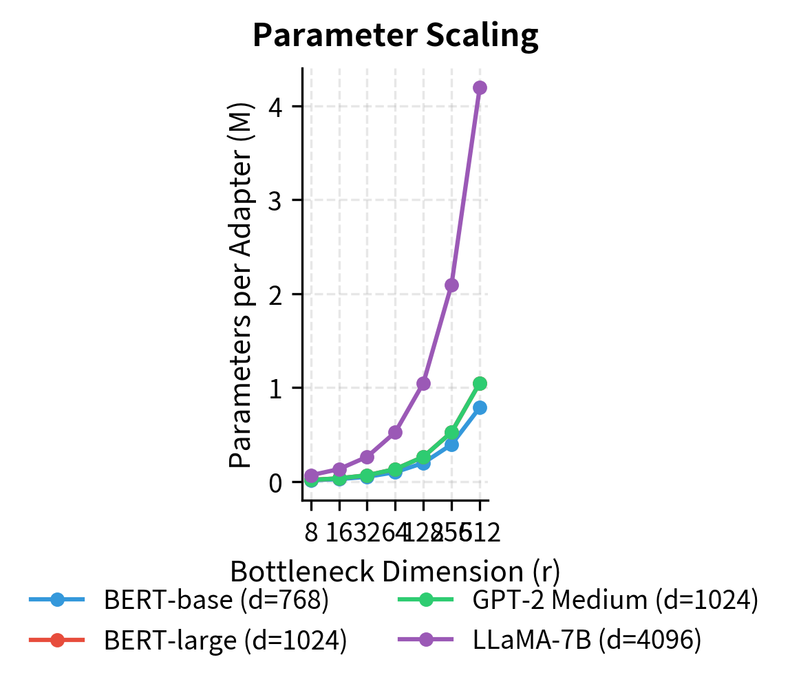
Scaling with Model Size
You should consider how to scale adapter dimensions as model size increases. Larger models have larger hidden dimensions, so maintaining the same absolute bottleneck size results in increasingly severe compression. A useful heuristic is to maintain a consistent compression ratio . For example:
However, empirical tuning often reveals that smaller models need proportionally larger adapters than bigger models. This may relate to the observation that larger models have more redundant capacity and can express task-specific information more compactly. A 7-billion parameter model has learned richer internal representations that can more easily be combined and adjusted through a small adapter, while a smaller model may require more adapter capacity to achieve the same effect.
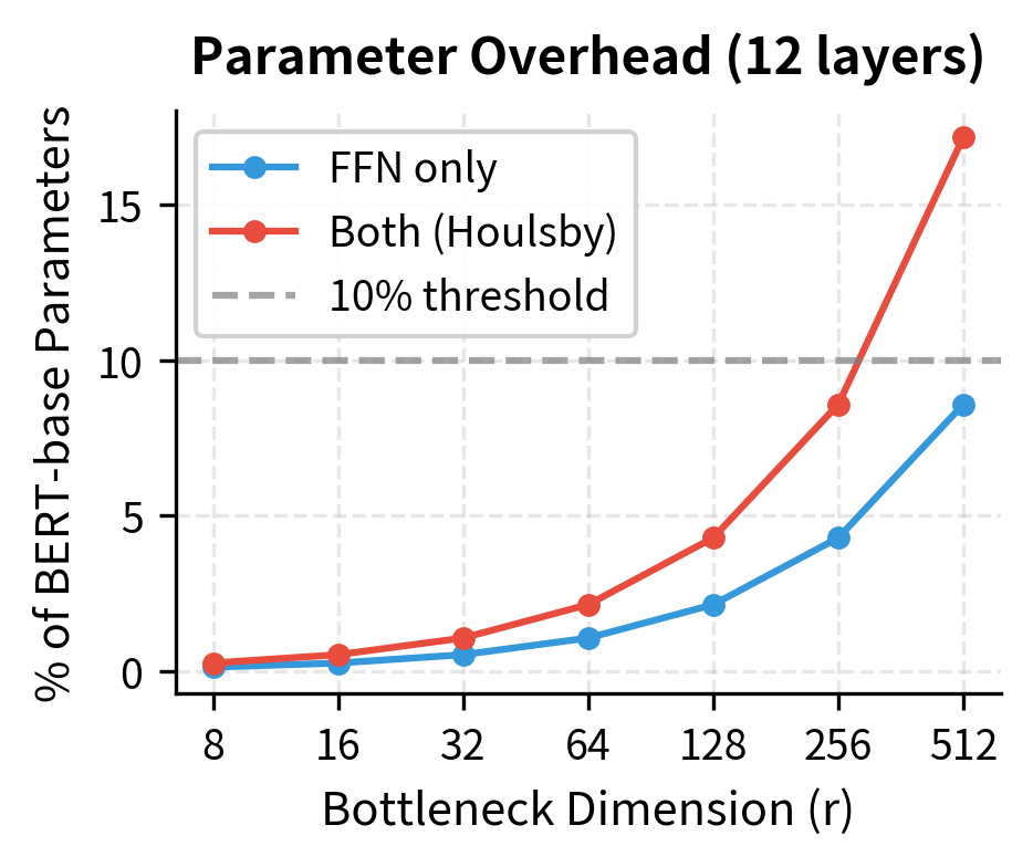
Adapter Efficiency Analysis
Let's compare the parameter overhead of adapters at different bottleneck dimensions for a BERT-base model with 12 layers and hidden dimension 768:
| Bottleneck Dim | Params per Adapter | Total Adapter Params | % of BERT-base |
|---|---|---|---|
| 8 | ~12K | ~288K | 0.26% |
| 32 | ~49K | ~1.2M | 1.1% |
| 64 | ~98K | ~2.4M | 2.2% |
| 256 | ~393K | ~9.4M | 8.6% |
Even at , adapters add less than 10% of the base model's parameters. This efficiency enables practical storage of dozens of task-specific adapters alongside a single frozen base model. For organizations deploying models across many tasks, this represents substantial savings in storage, memory, and model management overhead compared to maintaining separate fully fine-tuned models for each task.
Worked Example\n\nLet's trace through an adapter computation manually to build intuition for how the bottleneck transformation works. Following the computation step by step reveals how each component contributes to the final output and helps clarify the mathematical operations involved.
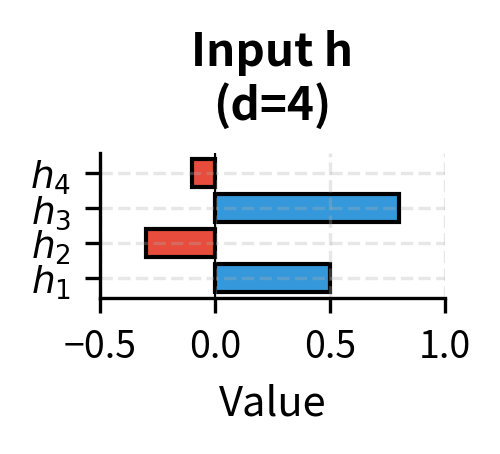
Consider a simplified scenario with hidden dimension and bottleneck dimension . While real adapters operate in much higher dimensions, this small example allows us to see every number in the computation. We have an input hidden state:
Our adapter has the following weights (after training). In practice, these would be learned through gradient descent, but here we use fixed values to illustrate the computation:
Step 1: Down-projection
The first step compresses the 4-dimensional input to a 2-dimensional bottleneck representation. This linear transformation identifies which combinations of input features are relevant for the task:
where:
- : the compressed bottleneck representation, which must encode all task-relevant information in just 2 dimensions
- : the down-projection weight matrix, whose rows define the feature combinations to extract
- : the input hidden state from the transformer
- : the bias vector that shifts the compressed representation
Computing the matrix-vector product by taking the dot product of each row of the weight matrix with the input vector:
Adding the bias to shift the representation:
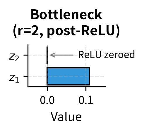
Step 2: Nonlinearity (ReLU)
The activation function introduces nonlinearity, allowing the adapter to model complex patterns. ReLU zeroes out negative values while passing positive values unchanged:
Notice that the second dimension is zeroed by ReLU, demonstrating how the activation function introduces sparsity. In this case, only one of the two bottleneck dimensions contributes to the output. This sparsity is a common feature of ReLU networks and can be seen as implicit feature selection within the bottleneck.
Step 3: Up-projection
The final transformation expands the activated bottleneck representation back to the original hidden dimension, producing the adapter's contribution to the final output:
where:
- : the output of the adapter, a 4-dimensional vector that will be added to the input
- : the up-projection weight matrix, whose columns define how each bottleneck dimension contributes to each output dimension
- : the activation of the bottleneck representation, with the second dimension zeroed by ReLU
- : the up-projection bias vector, set to zero in this example
Since the second dimension of is zero, only the first column of contributes to the output:
Step 4: Residual connection
Finally, the adapter output is added to the original input through the residual connection. This addition combines the pretrained representation with the task-specific modification:
The adapter has made small, targeted adjustments to each dimension of the hidden state. The residual connection ensures these changes are additive modifications rather than complete replacements. Notice that the modifications are relatively small compared to the original values, which is typical for well-trained adapters that make surgical adjustments rather than wholesale changes to the representation.
Code Implementation
Let's implement adapter layers from scratch and then integrate them into a pretrained transformer model.
Building the Adapter Module
We'll start by implementing a single adapter module as a PyTorch module:
Let's verify our adapter module works correctly and count its parameters:
The adapter adds approximately 99,000 parameters, which is only about 0.09% of BERT-base's 110 million parameters. Notice that the output shape matches the input shape, preserving the hidden dimension.
Integrating Adapters into a Transformer Layer
Now let's create a modified transformer layer that includes adapters:
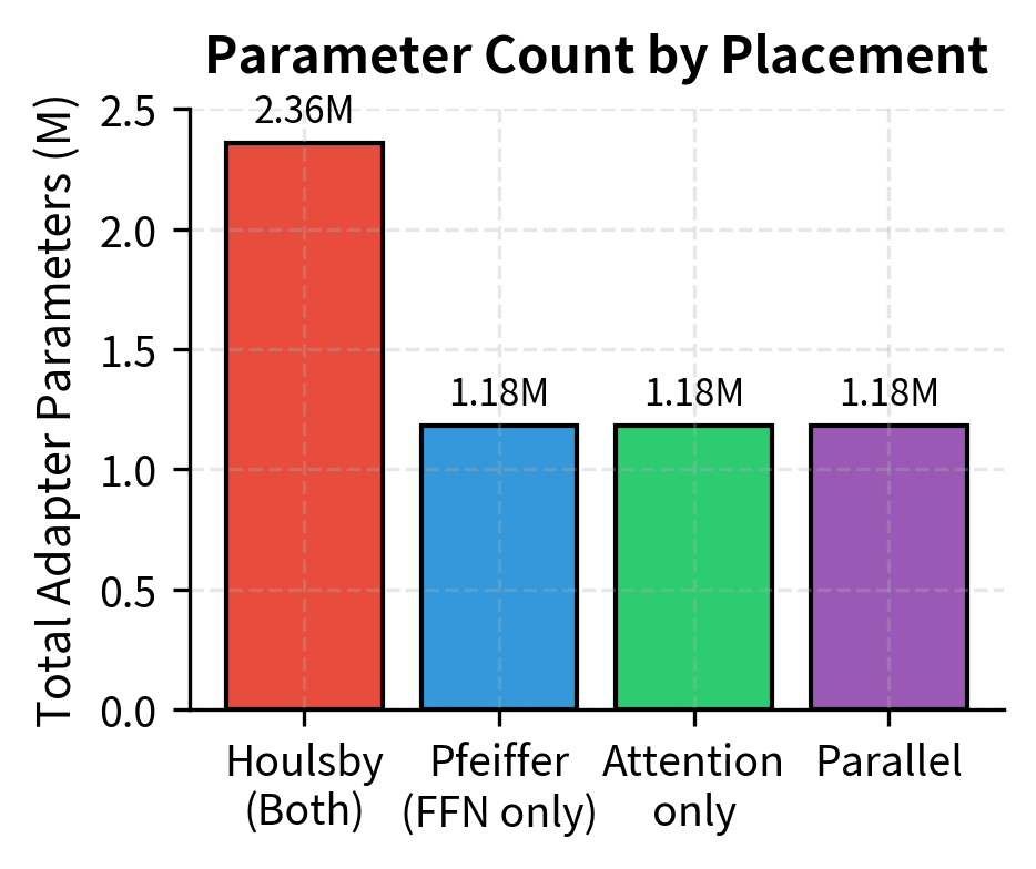
Let's compare parameter counts for different adapter placements:
The FFN-only placement uses half the adapter parameters while often achieving comparable performance to the original dual placement.
Freezing Pretrained Weights
A key aspect of adapter-based fine-tuning is keeping the pretrained weights frozen. Let's implement a utility to prepare a model for adapter training:
Only the adapter modules remain trainable, while all original transformer weights are frozen. This is the fundamental mechanism that enables parameter-efficient fine-tuning.
Visualizing Adapter Behavior
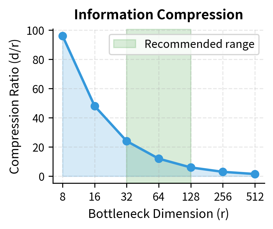
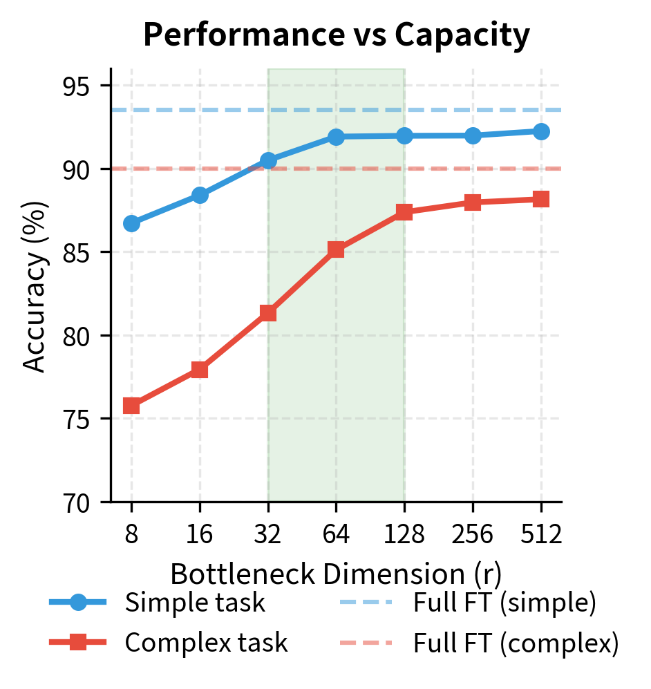
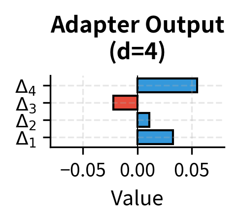
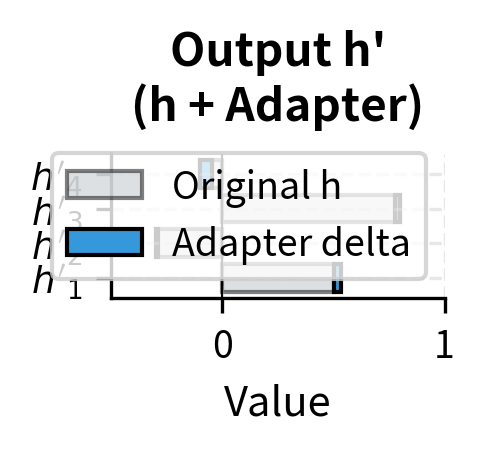
Let's visualize how an adapter transforms hidden representations during training:
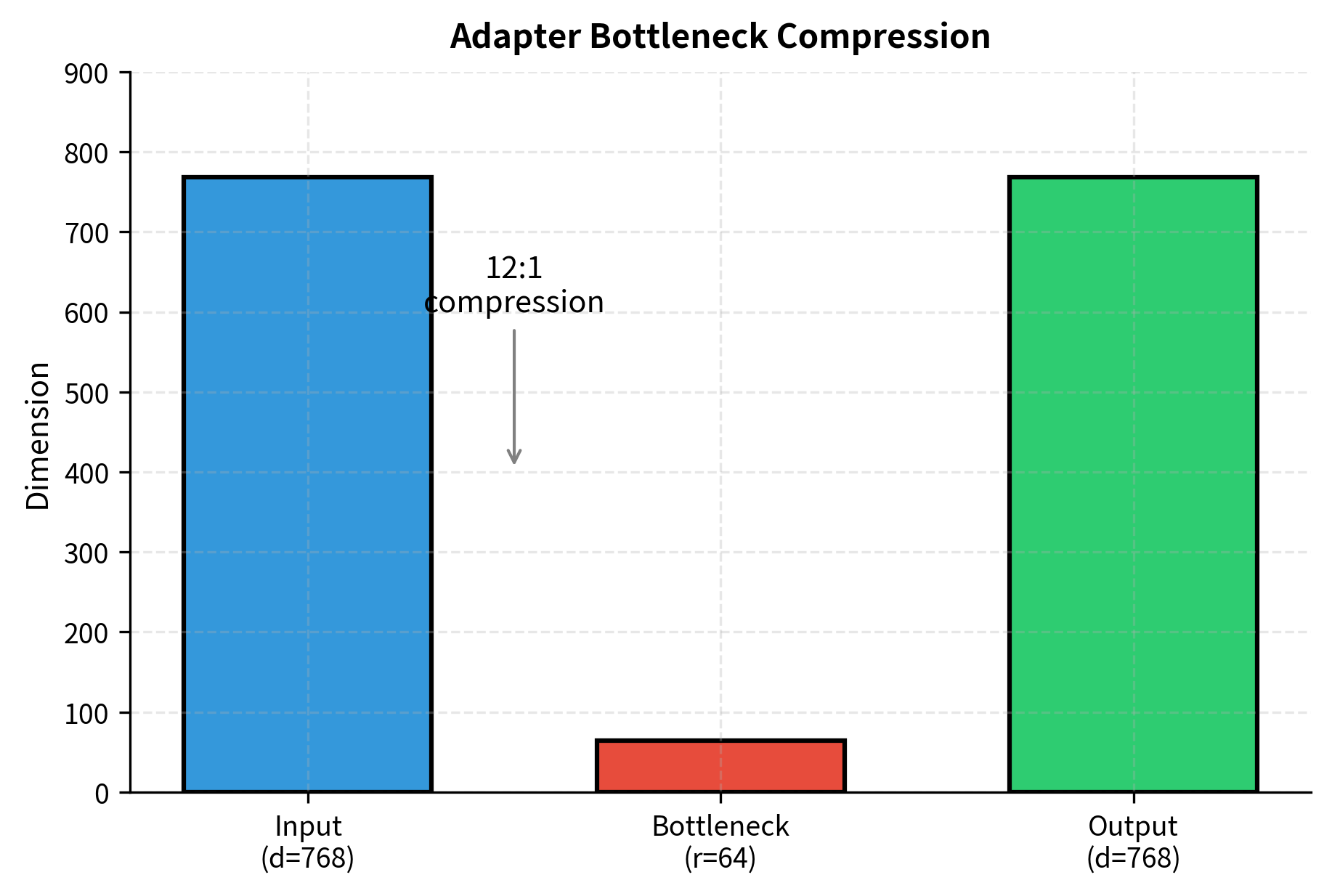
The visualization shows two key aspects of adapter behavior. The left panel illustrates the dramatic 12:1 compression ratio in the bottleneck, forcing the adapter to learn efficient encodings. The right panel shows how adapter outputs start near zero (due to our initialization strategy) and gradually increase as the adapter learns task-specific transformations.
Adapter Fusion
When you have multiple tasks and want a model that can handle all of them, you face a choice: train a single multi-task model, or train separate adapters for each task and combine them at inference time. Adapter fusion takes the second approach, providing a learned mechanism for combining multiple task-specific adapters. This technique enables flexible composition of specialized knowledge without the interference problems that often plague multi-task training.
The Multi-Adapter Challenge
Imagine you've trained separate adapters for sentiment analysis, named entity recognition, and question answering. Each adapter has learned to transform the base model's representations for its specific task, encoding knowledge about sentiment lexicons, entity boundaries, or answer extraction strategies. Now you encounter a task that requires reasoning about both sentiment and entities, such as analyzing customer reviews to identify which product features receive positive vs. negative sentiment.
Simple approaches like averaging adapter outputs often fail because different tasks may require emphasizing different adapters for different inputs. A token like "Apple" might need strong NER adapter influence to recognize it as an entity, while a token like "amazing" should draw primarily from the sentiment adapter. What you need is a learned attention mechanism that can dynamically weight adapter contributions based on the input context.
AdapterFusion Architecture
AdapterFusion introduces a fusion layer that combines the outputs of multiple pretrained adapters using attention. This approach treats the combination of adapters as itself a learning problem, where the model must discover how to best leverage each adapter's expertise for a new task.
Given task-specific adapters with outputs for input , the fusion layer computes a weighted combination:
Each term in this formula plays a specific role:
- : the combined output for the task, representing a learned mixture of all adapter contributions
- : the input hidden state, which provides context for determining how to weight the adapters
- : the attention weight for the -th adapter, indicating how much that adapter should contribute to this particular input
- : the value vector for the -th adapter, projected from the adapter output by . This projection allows the fusion layer to transform adapter outputs before combining them
- : the total number of task adapters being fused together
The attention weights are computed via a query-key-value attention mechanism, following the same pattern as the attention we studied in transformer architectures:
\alpha = \text{softmax}\left(\frac{\mathbf{Q} \cdot \mathbf{K}^T}{\sqrt{d_k}}\right) $$ this attention computation serves a specific purpose: - $\alpha$: the vector of attention weights across all adapters, summing to 1 due to the softmax normalization - $\text{softmax}$: the function normalizing the weights to sum to 1, ensuring the fusion produces a proper weighted average - $\mathbf{Q}$: the query derived from the hidden state, calculated as $\mathbf{h} \cdot \mathbf{W}_Q$. The query encodes "what kind of adapter output you are looking for?" - $\mathbf{K}$: the keys derived from adapter outputs, calculated as $[\mathbf{a}_i] \cdot \mathbf{W}_K$. Each key encodes "what kind of information does this adapter provide?" - $\sqrt{d_k}$: the scaling factor based on key dimension $d_k$ to stabilize gradients and prevent the softmax from producing overly peaked distributions The fusion weights $\mathbf{W}_Q$, $\mathbf{W}_K$, and $\mathbf{W}_V$ are the only new parameters trained during fusion. All adapter weights remain frozen, preserving the task-specific knowledge each adapter has learned while allowing the fusion mechanism to discover how to combine them effectively. ### Implementation Let's implement a basic adapter fusion layer:Let's test the fusion layer with simulated adapter outputs:
The fusion layer produces soft attention weights that sum to 1.0, allowing different adapters to contribute different amounts to the final output. These weights are learned during training on the target task.
Training Adapter Fusion
Adapter fusion uses a two-stage training process that preserves the knowledge in each individual adapter while learning how to combine them:
- Stage 1: Train individual adapters on their respective tasks with the base model frozen
- Stage 2: Train fusion layers with both the base model and individual adapters frozen
This separation ensures that adapter knowledge is preserved during fusion training. Only the small fusion parameters are updated in stage 2.
Visualizing Adapter Fusion
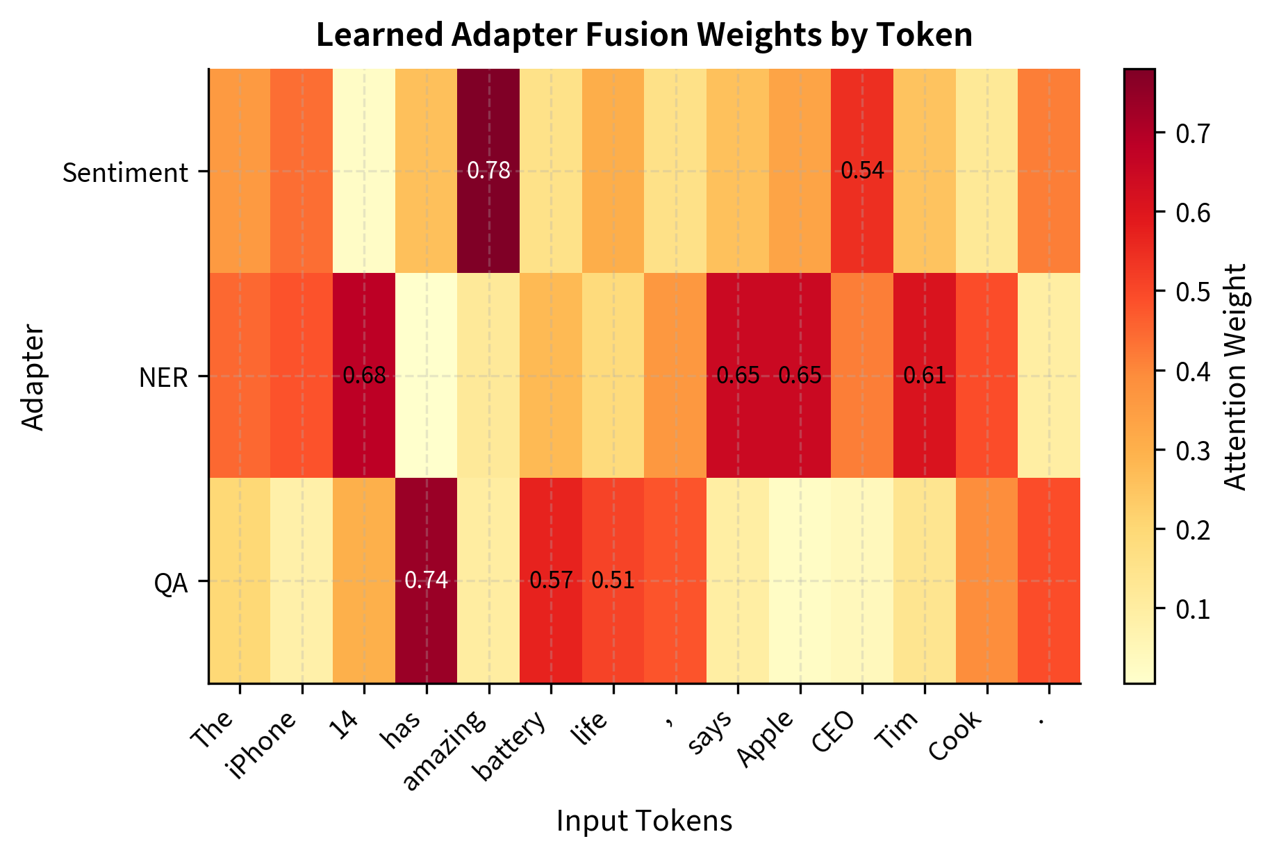
Let's visualize how fusion weights might vary across different input tokens:
The visualization shows how adapter fusion can learn meaningful attention patterns. Entity tokens like "Apple," "Tim," and "Cook" receive higher weights from the NER adapter, while opinion words like "amazing" activate the sentiment adapter more strongly.
Limitations and Impact
Adapter layers represented a significant advancement in parameter-efficient fine-tuning when introduced, establishing many concepts that influenced later methods like LoRA and prefix tuning. However, adapters come with their own set of trade-offs and limitations.
Inference Overhead
Unlike LoRA, which can merge its modifications into the base model weights after training, adapters must remain as separate modules during inference. Each forward pass through a transformer layer must also pass through the adapter modules, adding computational overhead. For a 12-layer model with dual adapters (Houlsby placement), this means 24 additional sequential operations per inference. While each adapter operation is small, the cumulative latency can become noticeable in latency-sensitive applications. This is particularly relevant when compared to LoRA, which we covered in earlier chapters of this part, where the low-rank modifications can be absorbed into the weight matrices for zero additional inference cost.
Sequential Dependencies
The sequential placement of adapters within the transformer forward pass limits parallelization opportunities. Modern hardware accelerators achieve peak efficiency when they can batch many operations together, but adapters introduce serial dependencies that can leave computational resources underutilized. Parallel adapter variants address this partially, but the fundamental architectural choice of inserting modules into the forward pass creates constraints that additive methods like LoRA avoid.
Activation Memory
During training, adapters require storing additional activations for backpropagation through their bottleneck layers. For large batch sizes or long sequences, this memory overhead can become significant. The bottleneck architecture mitigates this somewhat since the intermediate representation is small, but the input to each adapter (the full hidden state) must still be cached.
Historical Impact
Despite these limitations, adapters proved several important concepts that shaped the field:
- Additive fine-tuning works: The success of adapters demonstrated that pretrained models contain sufficient knowledge to adapt to new tasks with minimal additional parameters
- Bottleneck architecture: The compression-expansion pattern has been adopted and refined in many subsequent methods
- Modular adaptation: The idea of swappable, task-specific modules enabled new deployment patterns and influenced the development of mixture-of-experts approaches
- Adapter libraries: The need to manage multiple adapters catalyzed the development of tools like the Hugging Face PEFT library, which now supports many parameter-efficient methods
Adapter fusion particularly influenced the multi-task learning literature, showing that separately trained adaptations could be effectively combined without catastrophic interference between tasks.
Summary
This chapter explored adapter layers as a parameter-efficient approach to fine-tuning pretrained language models. We covered several key concepts:
Adapter architecture uses a bottleneck design where a down-projection compresses the hidden representation, a nonlinearity enables complex transformations, and an up-projection restores the original dimension. The residual connection around this bottleneck allows adapters to learn task-specific modifications while preserving the base model's representations.
Adapter placement can follow the original Houlsby strategy (adapters after both attention and FFN sublayers) or the more efficient Pfeiffer approach (adapters only after the FFN). The single-adapter placement often achieves comparable performance with half the parameters.
Adapter dimensionality controls the trade-off between capacity and efficiency. Bottleneck dimensions of 32 to 64 provide a good default for most tasks, with the compression ratio forcing adapters to learn generalizable transformations.
Adapter fusion enables combining multiple task-specific adapters through learned attention weights. This two-stage approach first trains individual adapters, then trains small fusion layers to dynamically weight their contributions.
Adapters add sequential inference overhead compared to methods like LoRA that can merge into base weights, but they offer clean modularity and established tooling. In the upcoming chapter on PEFT comparison, we'll examine how adapters stack up against the other methods we've covered, including LoRA variants, prefix tuning, and prompt tuning, across different tasks and model scales.
Quiz
Ready to test your understanding? Take this quick quiz to reinforce what you've learned about adapter layers and their role in parameter-efficient fine-tuning.

Comments