

Compare LoRA, QLoRA, Adapters, IA³, Prefix Tuning, and Prompt Tuning across efficiency, performance, and memory. Practical guide for choosing PEFT methods.

This article is part of the free-to-read Language AI Handbook
Choose your expertise level to adjust how many terms are explained. Beginners see more tooltips, experts see fewer to maintain reading flow. Hover over underlined terms for instant definitions.
PEFT Comparison
Throughout this part, we've explored six distinct approaches to parameter-efficient fine-tuning: LoRA, QLoRA, Adapters, IA³, Prefix Tuning, and Prompt Tuning. Each method introduces a different inductive bias about where task-specific knowledge should reside in a model. But when facing a new task, how do you choose which method to use?
This chapter synthesizes what we've learned into a practical comparison framework. We'll examine each method along multiple dimensions: parameter efficiency, task performance, computational overhead, and implementation complexity. By the end, you'll have concrete guidelines for selecting the right PEFT method for your specific use case.
Parameter Efficiency Comparison
PEFT methods adapt large models by updating only a small fraction of parameters. To compare these methods, we must establish concrete metrics. Examining the parameter counts reveals how methods differ in memory and storage requirements.
Absolute Parameter Counts
Let's establish concrete numbers for a typical 7B parameter model like LLaMA-2-7B with hidden dimension , 32 layers, and 32 attention heads. Calculating the parameters for each method shows the tradeoffs and suitability for different hardware constraints.
LoRA approximates weight updates by decomposing them into two low-rank matrices, and , such that . This design relies on the hypothesis that weight updates have a low "intrinsic rank," meaning the necessary adaptations exist in a low-dimensional subspace. The key insight motivating this approach is that while the original weight matrices are enormous, the changes needed to adapt a model to a new task may be far simpler in structure. If we can capture these changes using matrices with reduced dimensionality, we achieve massive parameter savings without sacrificing the model's ability to learn the task. For a layer with hidden dimension and rank , the number of parameters is . When applied to all four attention projections ():
The total number of trainable parameters for LoRA is calculated by summing the parameters of the low-rank matrices and across all target modules and layers. This calculation reveals how the rank parameter serves as a direct control knob for the tradeoff between model capacity and parameter count:
where:
- : the number of target modules per layer (Query, Key, Value, Output)
- : parameters for matrices and in one module (since each has size or )
- : hidden dimension ()
- : rank of the low-rank adapters ()
- : number of layers ()
For our LLaMA-2-7B configuration, this yields:
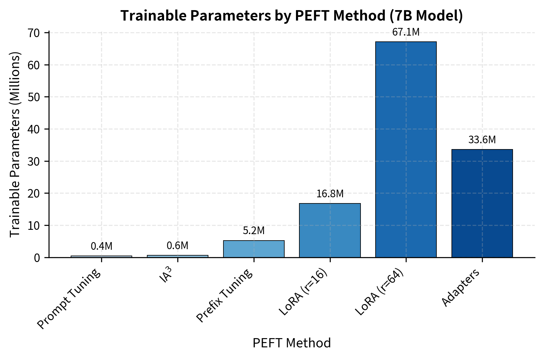
This result is striking: we can adapt a 7 billion parameter model by training only 16.8 million parameters, a reduction of over 400 times. The rank of 16 is deliberately chosen to be small enough to provide substantial parameter savings while still offering sufficient capacity for most adaptation tasks.
Adapters insert bottleneck modules (consisting of a down-projection and an up-projection) after both the attention and feed-forward (FFN) layers. This bottleneck architecture compresses inputs into a lower-dimensional representation before expanding them back, reducing parameter count while enabling non-linear adaptation. The fundamental idea behind adapters is that task-specific information can be "filtered" through a narrow bottleneck, forcing the model to learn only the most essential transformations. This compression-expansion pattern also introduces non-linearity through activation functions, giving adapters additional representational power compared to linear methods like LoRA. With bottleneck dimension :
We calculate the parameter count by summing the weights of the down-projection and up-projection matrices for each adapter. The symmetry of this calculation, with equal contributions from each projection direction, reflects the balanced nature of the bottleneck design:
where:
- : the number of adapters per layer (one inserted after Attention, one after FFN)
- : the hidden dimension of the model ()
- : the size of the bottleneck dimension ()
- : the number of parameters in the down-projection matrix
- : the number of parameters in the up-projection matrix
- : the number of layers in the model ()
Plugging in the values:
Adapters require roughly twice as many parameters as LoRA with rank 16. This increased parameter count buys additional expressiveness through the non-linear activation function between the down and up projections, but comes at the cost of both storage and, as we'll see later, inference overhead.
Prefix Tuning prepends learnable vectors to the keys and values at every layer. These virtual tokens effectively "steer" the attention mechanism at every depth, guiding the model's internal processing. Rather than modifying the model's weights directly, prefix tuning modifies the context that the model attends to. Optimizing key-value pairs at every layer influences attention flow without changing the transformation matrices. With prefix length :
The trainable parameters consist of the virtual token embeddings added to the Key and Value matrices at each layer. This formulation makes clear why prefix tuning affects only the attention mechanism: we're adding content for the model to attend to, not modifying how it processes that content:
where:
- : the prefix length (number of virtual tokens, set to )
- : the hidden dimension ()
- : a factor accounting for application to both Key and Value matrices
- : the number of layers ()
Substituting the values:
The parameter count for Prefix Tuning is lower than LoRA despite operating at every layer. This efficiency comes from the method's focused scope: it only influences the attention mechanism through the key-value channel, leaving all other computations unchanged.
Prompt Tuning adds learnable embeddings only at the input layer. Unlike discrete text prompts, these continuous embeddings are optimized directly via backpropagation to find the most effective task trigger. This approach represents perhaps the simplest possible form of model adaptation: we're essentially learning a better way to "ask" the model to perform our task. The continuous nature of these embeddings allows optimization to find representations that may have no natural language equivalent, potentially discovering more effective task specifications than any human-written prompt could provide. With prompt length :
The parameters come solely from the learnable embeddings prepended to the input layer. This single-layer application is what gives Prompt Tuning its remarkable parameter efficiency, though it also limits the method's ability to influence deep model computations:
where:
- : the prompt length (number of virtual tokens, set to )
- : the embedding dimension ()
Calculating the total:
With fewer than half a million parameters, Prompt Tuning achieves the smallest footprint of any method we've examined. This extreme efficiency makes it ideal for scenarios where storage or memory is at an absolute premium, though as we'll see in the performance analysis, this efficiency comes with tradeoffs.
IA³ introduces learned vectors that scale the activations element-wise. This acts like a feature equalizer, selectively amplifying or suppressing specific activation channels. IA³ assumes the base model computes useful features and only needs to adjust their relative importance for different tasks. Rather than learning new transformations, IA³ learns which existing computations to emphasize and which to diminish. IA³ is effective because it leverages pre-trained representations. We calculate the parameter count by summing the scaling vectors for the Key, Value, and FFN intermediate activations:
where:
- : the dimension of scaling vectors for attention keys and values (, matching the hidden dimension)
- : the dimension of the scaling vector for the FFN expansion layer ()
- : the number of layers ()
This results in a very small number of parameters:
The parameter count for IA³ is remarkably low, just over half a million for a 7B model. This efficiency stems from the element-wise nature of the scaling operation: we need only one scalar per activation dimension, rather than full transformation matrices. The tradeoff is that IA³ can only rescale existing activations, not compute fundamentally new features.
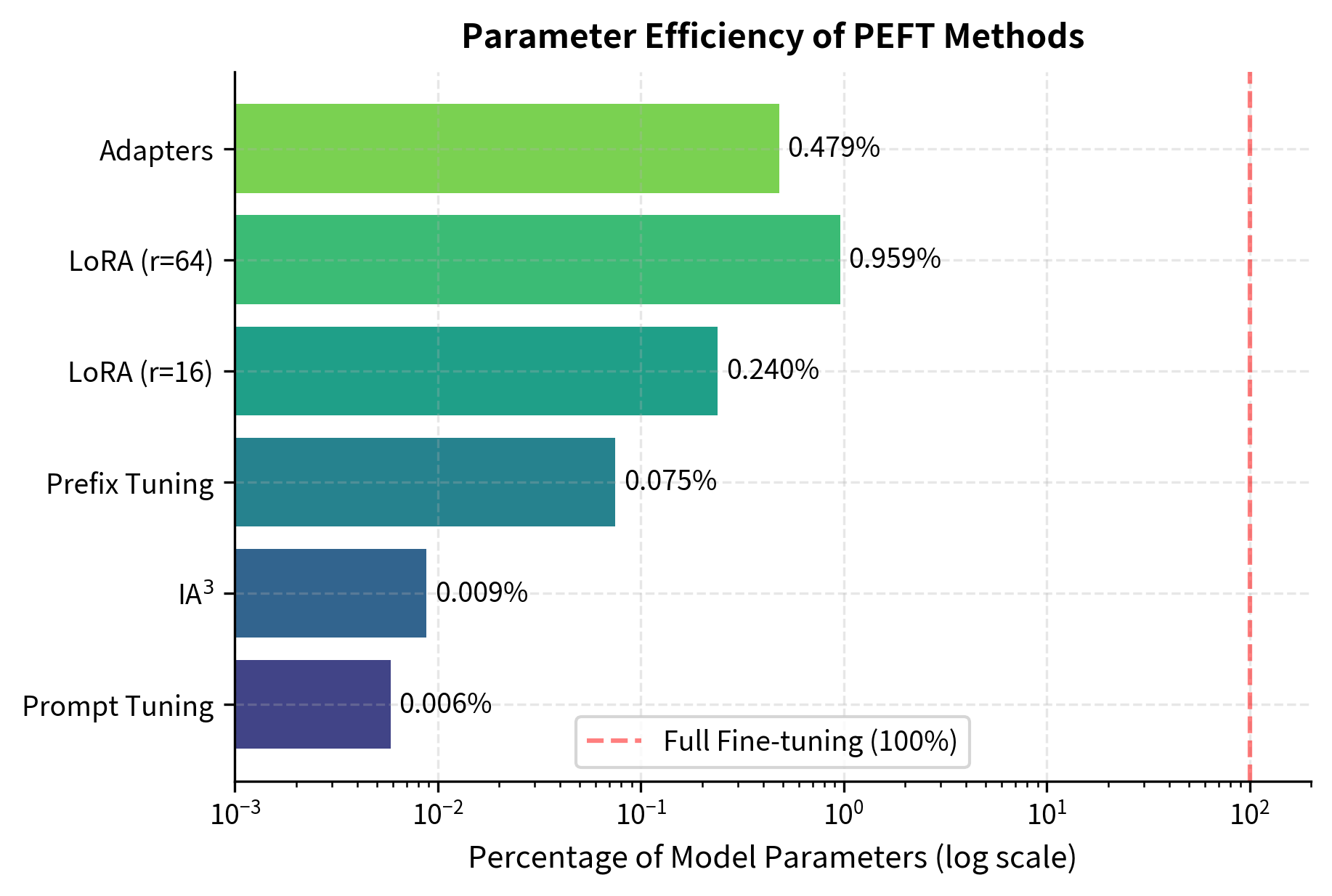
The differences are dramatic. Prompt Tuning and IA³ train fewer than 1 million parameters, less than 0.01% of the model. LoRA at typical ranks trains 0.2-0.9% of parameters. Even the "heaviest" PEFT method (Adapters) trains less than 0.5% of the model. These numbers illustrate a fundamental principle: the vast majority of a pre-trained model's knowledge is encoded in its frozen weights, and task-specific adaptation can be achieved with remarkably few additional parameters.
Memory Footprint Analysis
Parameter count alone doesn't tell the full story. During training, memory consumption includes model weights, optimizer states, gradients, and activations. Understanding the complete memory picture is essential for determining which methods will actually fit on your hardware. A method might train fewer parameters but still require substantial memory for other components of the training process.
For full fine-tuning with AdamW, memory is consumed by weights, optimizer states, gradients, and activations. Assuming mixed precision training:
We calculate the memory requirements by summing the components needed for model states and training overhead. This includes the static footprint of the model weights and the dynamic memory required for optimizer states, gradients, and forward-pass activations. Each component plays a distinct role in the training process, and understanding their individual contributions helps explain why full fine-tuning is so memory-intensive:
where:
- weights: memory for the model parameters (usually FP16)
- optimizer: memory for optimizer states (like momentum and variance in AdamW)
- gradients: memory for storing gradients during backpropagation
- activations: memory for intermediate outputs needed for the backward pass
Using a simplified estimation model:
where:
- : the total number of model parameters
- : FP16 model weights ( bytes per parameter)
- : optimizer states (simplified estimate)
- : gradients (FP32 or mixed)
- : activations (approximate average)
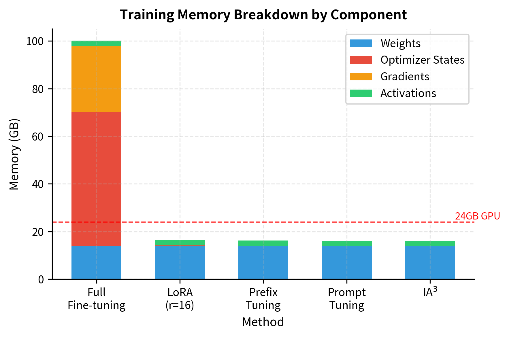
A 7B model requires approximately 84 GB of VRAM. Full fine-tuning is memory-intensive because requirements scale linearly with parameters, and each parameter needs storage for multiple values.
PEFT methods drastically reduce memory by freezing the base model and training only the adapter parameters. The key insight is that frozen parameters need only their weights stored, not optimizer states or gradients. With LoRA (rank 16):
For LoRA, we only need to store the optimizer states and gradients for the small set of trainable parameters, while the base model remains frozen in low precision. This separation between frozen and trainable parameters is the fundamental mechanism through which all PEFT methods achieve their memory efficiency:
where:
- : the number of frozen base model parameters ( billion)
- : the number of trainable LoRA parameters ( million)
- : bytes per frozen parameter (FP16 weights only)
- : the memory factor for trainable parameters (weights + optimizer + gradients + activations)
Applying this to our example:
This is why a 7B model that requires 80+ GB for full fine-tuning can be fine-tuned with LoRA on a single 24GB GPU. Memory savings make fine-tuning accessible; LoRA enables adaptation on hardware unsuitable for full fine-tuning. This shift in memory requirements enables you to adapt large models for your specific needs without expensive compute clusters.
The estimated values demonstrate the massive efficiency gains of PEFT. While full fine-tuning demands over 80GB of VRAM, requiring high-end data center GPUs, all PEFT methods operate comfortably within the memory limits of consumer hardware (14-16GB). This 5-6x reduction in memory footprint is what makes fine-tuning more accessible. The practical implication is transformative: techniques that were once exclusive to well-funded research labs are now available to you, small teams, and educational institutions.
Performance Comparison Across Tasks
Parameter efficiency means nothing if the method doesn't work. Let's examine how these methods perform across different task categories. We will examine how performance varies across tasks and data sizes to inform your selection guidelines.
Natural Language Understanding
NLU tasks like sentiment analysis, natural language inference, and question answering have been extensively benchmarked. Classification and extraction tasks are the most studied PEFT domains and provide robust comparative data. On the GLUE benchmark, the relative ordering tends to be:
Full Fine-tuning ≥ LoRA ≥ Adapters ≥ IA³ > Prefix Tuning > Prompt Tuning
However, the gaps are often smaller than you might expect. The methods that train more parameters (LoRA, Adapters) achieve performance closer to full fine-tuning, while the ultra-efficient methods (Prompt Tuning, IA³) show somewhat larger gaps. Yet even the "weakest" PEFT methods often achieve respectable performance. On BERT-base with the standard GLUE tasks:

The key insight: LoRA typically achieves 95-99% of full fine-tuning performance while training less than 1% of parameters. This remarkable efficiency ratio is what makes PEFT methods so attractive for practical applications. You can often get nearly all the benefit of full fine-tuning at a tiny fraction of the cost. The performance gap between LoRA and full fine-tuning on these NLU tasks is often within the noise of hyperparameter selection, suggesting that for many classification tasks, LoRA represents a near-optimal tradeoff between efficiency and capability.
Natural Language Generation
Generation tasks, such as summarization, translation, and dialogue, show different patterns. The quality of generated text depends heavily on how well the method can modify the model's output distribution. Generation tasks are sensitive to adaptation quality because they require sequential predictions where small errors compound.
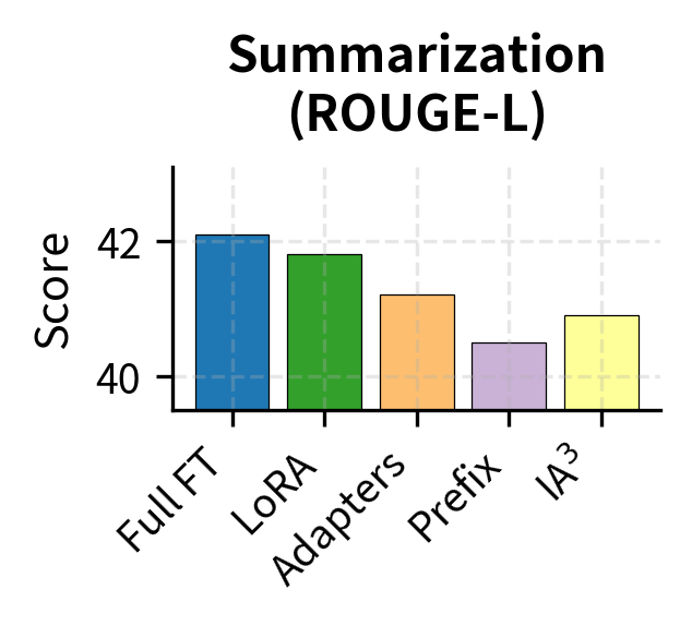
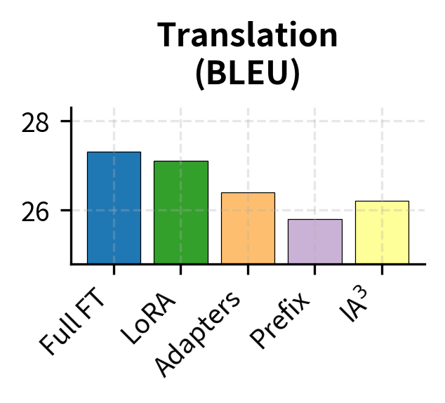
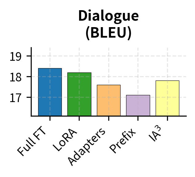
Prefix Tuning shows a larger gap on generation tasks. This makes intuitive sense: as we discussed in the Prefix Tuning chapter, the method modifies attention patterns through prefix keys and values but doesn't directly alter how the model generates output tokens. The feed-forward networks, which play a crucial role in transforming attended information into next-token predictions, remain entirely unchanged by prefix tuning. LoRA, by contrast, can modify both the attention mechanism and (when applied appropriately) the FFN layers, giving it more direct control over the generation process.
Instruction Following and Chat
The most practical application of PEFT today is adapting base models to follow instructions. This presents a unique challenge: the model must learn both the format of instruction-response pairs and diverse task knowledge. Instruction following requires the model to understand when it should generate output, what style that output should take, and how to appropriately respond to the vast diversity of your requests. This multi-faceted learning objective places significant demands on the adaptation method's capacity.
On instruction-following benchmarks, LoRA-tuned models often match fully fine-tuned versions:
QLoRA's strong performance here is remarkable: it achieves near-LoRA quality while enabling fine-tuning of 7B models on consumer GPUs with just 24GB of memory. The combination of 4-bit quantization for the base model weights and full-precision LoRA adapters proves to be an excellent practical compromise. We'll explore instruction tuning in depth in the next part.
Few-Shot and Low-Resource Settings
When training data is scarce (hundreds rather than thousands of examples), the relative performance of methods shifts. Data efficiency becomes a critical concern when labeled examples are expensive to obtain, when working with specialized domains, or when rapidly prototyping new applications. Understanding how each method behaves in low-data regimes helps inform decisions about whether to invest in data collection or accept the performance tradeoffs of a more efficient method:
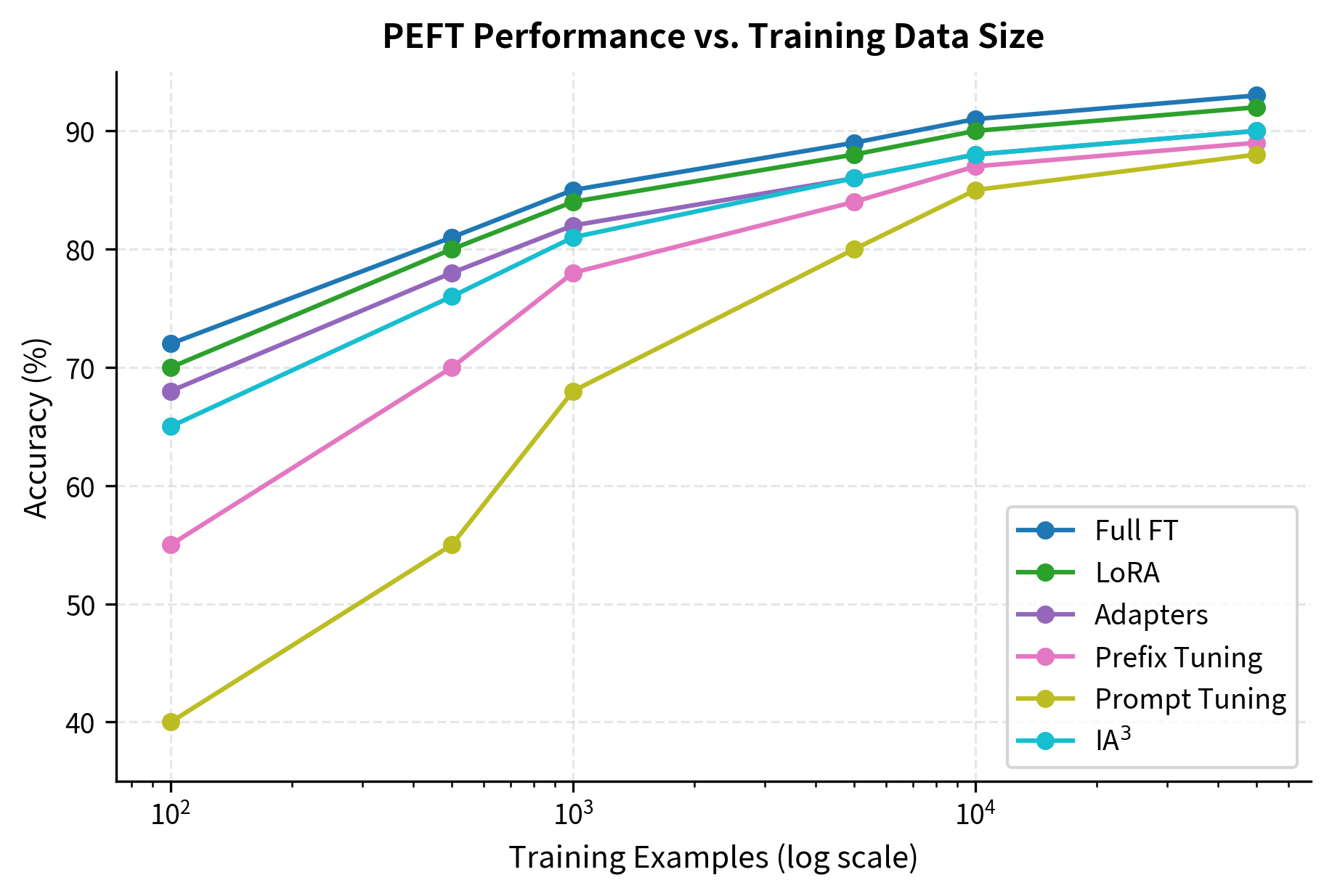
The pattern is clear: methods that train more parameters (LoRA, Adapters) are more data-hungry but achieve higher peak performance. Prompt Tuning struggles with limited data because it must learn rich representations from scratch in a very low-dimensional space. The soft prompt embeddings start as random vectors with no task-relevant structure, and with only a few hundred examples, there simply isn't enough signal to learn effective representations. IA³, while also parameter-efficient, fares better in low-data settings because its scaling approach builds on the model's existing feature representations rather than learning new ones from scratch.
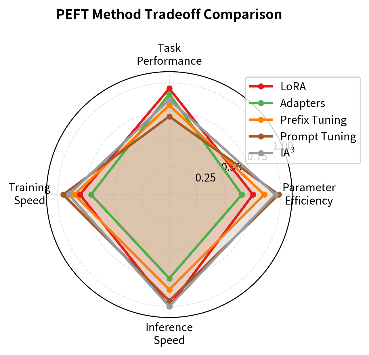
Computational Overhead Analysis
Beyond memory, PEFT methods differ in their computational costs during training and inference. These differences can significantly impact both development iteration speed and production serving costs. A complete understanding of PEFT tradeoffs requires examining not just parameter counts and performance, but also the time and compute required to train and deploy adapted models.
Training Speed
Training throughput depends on several factors that interact in complex ways:
- Forward pass overhead: Added computation from adapter layers or modified attention. Methods that introduce new layers (Adapters) or extend sequence length (Prefix Tuning) increase forward pass time.
- Backward pass scope: How many parameters receive gradients. Methods with fewer trainable parameters compute fewer gradients, reducing backward pass time significantly.
- Memory access patterns: Sequential access (Adapters) vs. broadcasted scaling (IA³). Memory-efficient operations can provide substantial speedups even when parameter counts are similar.
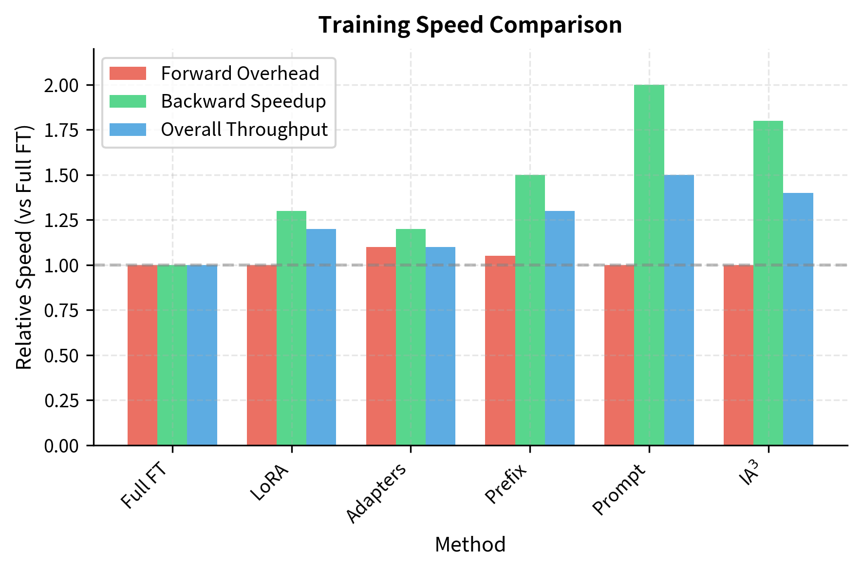
Throughput improves primarily from reduced gradient computation. Prompt Tuning is fastest because gradients flow through only 100 embedding vectors. The backward pass is faster because most parameters are frozen.
Inference Impact
A critical distinction: some PEFT methods add inference overhead while others are "free" at inference time. This distinction has major implications for production deployments, where inference costs often dominate the total cost of ownership for ML systems.
Zero inference overhead:
- LoRA: Weights can be merged () after training. The low-rank decomposition is purely a training-time construct; once the adapter is trained, we can precompute the full weight update and fold it into the base model weights.
- IA³: Scaling can be folded into weights. Since IA³ applies element-wise multiplication, the scaling factors can be absorbed into the preceding linear transformation's weights.
- Prompt Tuning: Only adds constant prefix tokens (minimal impact). While there is a small increase in sequence length, this typically adds less than 5% to inference time.
Persistent inference overhead:
- Adapters: Must execute additional layers at every forward pass. The bottleneck computations cannot be removed because they involve non-linear activations that cannot be merged with surrounding linear operations.
- Prefix Tuning: Increases effective sequence length by prefix size. The prefix tokens add to the key-value cache and increase attention computation proportional to the prefix length.
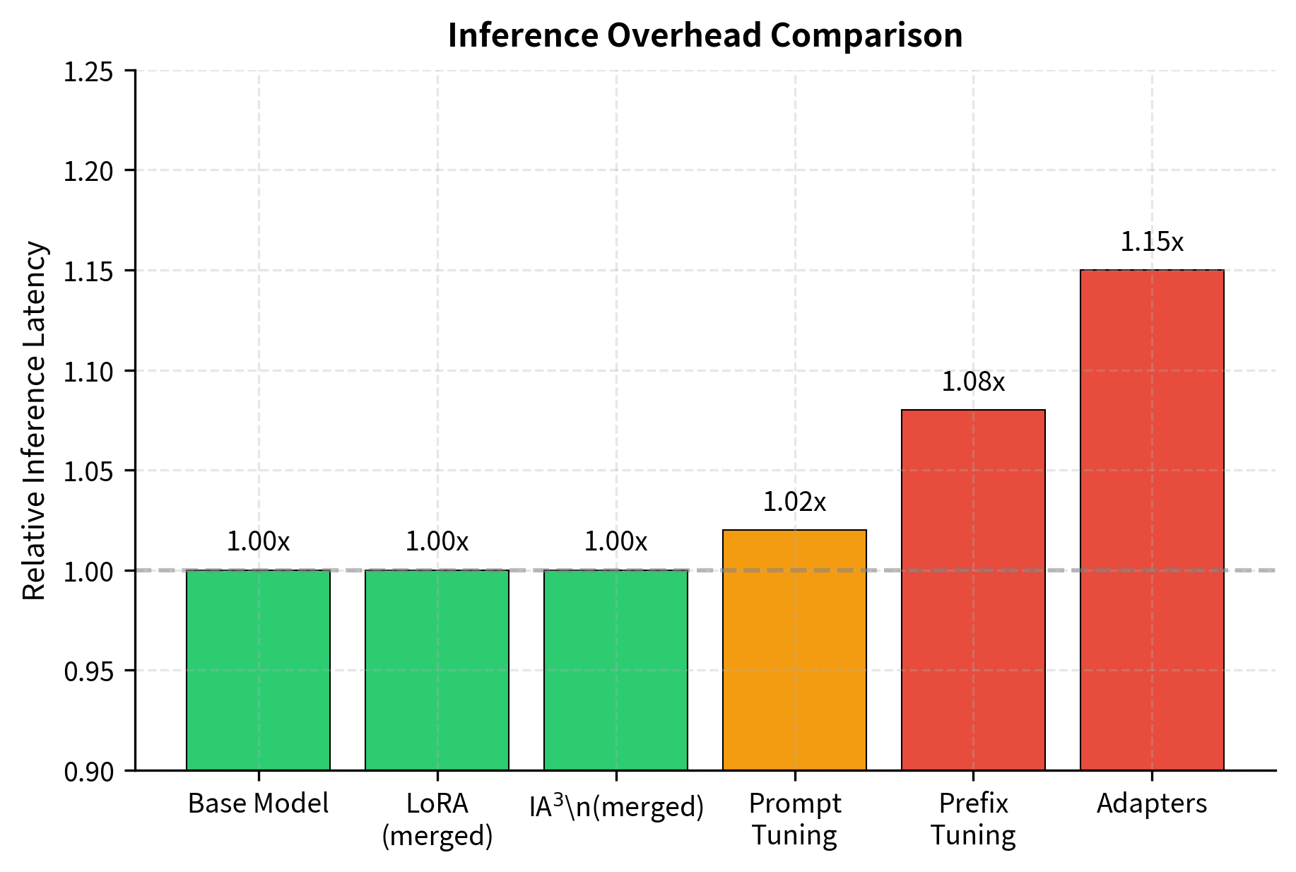
For production deployments where inference cost dominates, LoRA's ability to merge weights is a significant advantage. You get the benefits of task-specific adaptation with identical serving costs to the base model. This property makes LoRA the preferred choice for applications where models must serve millions of requests, as even small percentage increases in latency translate to substantial infrastructure costs at scale.
Task Suitability Analysis
Different PEFT methods suit different scenarios. Let's map methods to use cases based on the technical properties we've analyzed. The goal is to provide actionable guidance that accounts for your specific constraints and requirements. No single method is universally best; the right choice depends on your particular combination of performance needs, resource constraints, and deployment requirements.
When to Use LoRA
LoRA is the default choice for most scenarios and excels when:
- You need maximum performance: LoRA consistently achieves the smallest gap to full fine-tuning across diverse task types and model scales
- Inference cost matters: Merged weights mean zero serving overhead, making LoRA ideal for high-traffic production deployments
- You're fine-tuning on GPUs with 24-48GB VRAM: Standard LoRA (r=16-64) fits comfortably on professional-grade consumer hardware
- You want to stack multiple adapters: Different LoRA weights can be loaded dynamically for multi-task serving, enabling efficient model customization without maintaining separate model copies
Avoid LoRA when:
- You have fewer than 100 training examples (consider few-shot prompting instead)
- Memory is severely constrained (consider QLoRA or Prompt Tuning)
When to Use QLoRA
QLoRA extends LoRA's applicability to memory-constrained settings by combining 4-bit quantization of base model weights with standard LoRA adapters:
- Consumer hardware: Fine-tune 7B models on 24GB GPUs, 13B on 48GB, making large model adaptation accessible without enterprise-grade hardware
- Large models on limited budgets: Access to 70B-scale models without A100 clusters, democratizing research on frontier-scale models
- Research and experimentation: Lower barrier to entry for exploring large models, enabling faster iteration during the exploratory phase of projects
Avoid QLoRA when:
- Training speed is critical (quantization adds ~10-20% overhead due to the need to dequantize weights during computation)
- You have access to more memory (standard LoRA trains faster and avoids any potential quality degradation from quantization)
When to Use Adapters
Adapters are well-suited for scenarios that benefit from their modular, plug-and-play architecture:
- Multi-task learning: Each task gets its own adapter module, enabling clean separation of task-specific knowledge
- Modular architectures: Adapters compose naturally (task adapter + language adapter), allowing hierarchical organization of model capabilities
- Interpretability research: Adapter outputs can be probed to understand task-specific processing, as the discrete adapter boundaries provide natural intervention points
Avoid Adapters when:
- Inference latency is critical (adapters add permanent overhead that cannot be eliminated through weight merging)
- Maximum parameter efficiency is required (adapters train more parameters than LoRA at comparable performance levels)
When to Use Prefix Tuning
Prefix Tuning works well for scenarios that align with its attention-based modification approach:
- NLG tasks: Especially controllable generation where prefix vectors can encode style/tone attributes without modifying the core generation mechanism
- Interpretability: Prefix attention patterns reveal what the model "looks for," as you can analyze which positions in the prefix receive attention for different inputs
- Moderate data regimes: Better data efficiency than Prompt Tuning due to per-layer parameterization, while still more efficient than LoRA or Adapters
Avoid Prefix Tuning when:
- You're working with very long contexts (prefix reduces effective context length, potentially cutting into your input budget)
- Tasks require modifying feed-forward computation (prefix only affects attention, leaving FFN layers entirely unchanged)
When to Use Prompt Tuning
Prompt Tuning is the simplest PEFT method and fits scenarios where extreme efficiency is paramount:
- Extremely large models: When you can only access models through APIs or when even inference-only deployment is challenging
- Maximum parameter efficiency: Less than 0.01% trainable parameters, enabling storage of thousands of task-specific adaptations
- Large-scale multi-tenancy: Your tuned prompt is tiny to store, making personalized model adaptations economically feasible at scale
Avoid Prompt Tuning when:
- Training data is limited (Prompt Tuning is data-hungry, requiring thousands of examples to achieve good performance)
- Tasks require significant behavioral change from base model (the limited parameter budget constrains adaptation capacity)
- You need interpretable adaptations (soft prompts are not human-readable and resist straightforward analysis)
When to Use IA³
IA³ offers a unique balance between efficiency and capability through its activation scaling approach:
- Few-shot settings: Better data efficiency than Prompt Tuning because it builds on existing representations rather than learning from scratch
- Minimal overhead: Scales apply through element-wise multiplication, which is computationally trivial and adds no inference latency when folded into weights
- Quick experiments: Fastest to train among methods that modify attention, enabling rapid prototyping and ablation studies
Avoid IA³ when:
- Maximum performance is required (typically 1-2% below LoRA on most benchmarks)
- The task requires learning entirely new capabilities (limited expressiveness constrains what the model can learn)
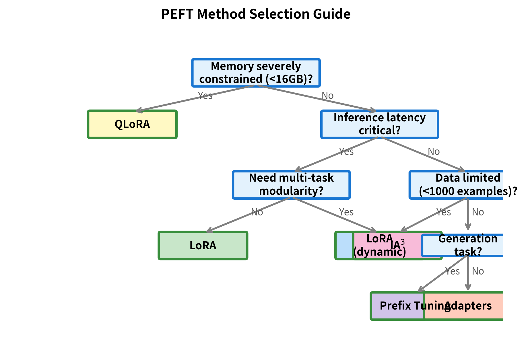
Practical Recommendations
Based on the analyses above, here are concrete recommendations for common scenarios:
General-Purpose Fine-tuning
If you are fine-tuning LLMs for downstream tasks:
- Start with LoRA (, ) applied to all attention projections
- Use 4-bit QLoRA if you're GPU-memory constrained
- Increase rank to 32-64 if performance is insufficient
- Add FFN adaptation (LoRA on up/down projections) for tasks requiring significant behavioral change
Production Deployment
When serving fine-tuned models in production:
- Merge LoRA weights into base model for zero inference overhead
- Avoid Adapters unless you need runtime adapter switching
- For multi-tenant serving: Keep LoRA weights separate and apply at runtime with specialized serving infrastructure
Research and Experimentation
When exploring new tasks or model capabilities:
- Start with Prompt Tuning for fastest iteration
- Move to IA³ if Prompt Tuning underperforms
- Use LoRA for final experiments requiring best performance
Extreme Resource Constraints
When working with very limited compute:
- QLoRA with provides excellent efficiency
- Gradient checkpointing trades compute for memory
- Consider API-based fine-tuning if available for your model
Implementation: Comparative Analysis
Let's implement a framework for comparing PEFT methods on a real task.
These results confirm the theoretical efficiency of PEFT. Prompt Tuning uses under 0.01% of parameters, while LoRA uses about 0.5%. This footprint enables the memory savings calculated from first principles.
Now let's measure training throughput:
Prompt Tuning and IA³ offer the highest training throughput, requiring gradients for only a small number of parameters. LoRA and Prefix Tuning also provide speedups over full fine-tuning, though the exact gain depends on the rank and number of adapted layers. These speed improvements, while less dramatic than the memory savings, significantly accelerate the iterative development cycle. Faster training means more experiments per day, faster hyperparameter searches, and quicker iteration toward optimal configurations.
Combining PEFT Methods
An emerging research direction explores combining multiple PEFT methods for improved performance. The intuition is that different methods modify different aspects of model behavior, and their complementary strengths might compound when combined:
LoRA + Adapters: Apply LoRA to attention layers and adapters after FFN layers. This captures both low-rank attention modifications and complex post-FFN transformations.
Prompt Tuning + LoRA: Use soft prompts for task-level conditioning while LoRA handles fine-grained adaptation. Particularly useful for instruction-following with multiple task types.
Key Parameters
The key configuration classes and parameters for PEFT methods are:
-
- r: Rank of the update matrices. Lower means fewer parameters and less memory.
- lora_alpha: Scaling factor for updates. The weight scaling is .
- target_modules: List of module names (e.g., "query", "value") to apply LoRA to.
- lora_dropout: Dropout probability for LoRA layers, aiding in regularization.
-
PrefixTuningConfig / PromptTuningConfig:
- num_virtual_tokens: Number of learnable tokens to prepend (prefix or prompt length).
- prompt_tuning_init: Initialization method for soft prompts (e.g., random or from text).
Limitations and When to Use Full Fine-tuning
Despite their efficiency, PEFT methods have inherent limitations:
Constrained adaptation capacity: By design, PEFT methods limit what the model can learn. For tasks requiring substantial behavioral change, such as learning a new language, acquiring domain expertise, or fundamentally shifting the model's capabilities, full fine-tuning may be necessary. LoRA's low-rank constraint assumes task-specific modifications live in a low-dimensional subspace, which may not hold for all tasks.
Degradation at scale: While PEFT methods work well for single-task adaptation, repeatedly applying multiple LoRA adapters or stacking adapters can lead to interference. Research on LoRA merging and multi-task adapter composition remains active.
Sensitivity to hyperparameters: PEFT methods introduce new hyperparameters (rank, prefix length, bottleneck dimension) that require tuning. Poor choices can significantly impact performance, sometimes more dramatically than learning rate selection in full fine-tuning.
Not a substitute for pre-training: PEFT methods adapt existing capabilities; they don't create new ones. A model that doesn't "know" something from pre-training generally won't learn it from PEFT alone, regardless of how much task-specific data you provide.
When should you opt for full fine-tuning despite the efficiency benefits of PEFT?
- Maximum performance is non-negotiable: In high-stakes applications, the 1-3% gap to full fine-tuning may matter
- Sufficient compute is available: If you have the resources, full fine-tuning remains the gold standard
- Task requires deep behavioral change: Domain adaptation, safety training, or capability unlocking may exceed PEFT's adaptation budget
- You're creating a foundation for further PEFT: Full fine-tuning a domain-specific base model, then using PEFT for downstream tasks
Summary
This chapter synthesized our exploration of parameter-efficient fine-tuning methods into practical guidance for method selection:
Parameter efficiency varies by orders of magnitude. Prompt Tuning and IA³ train fewer than 0.01% of parameters, while LoRA and Adapters train 0.2-0.5%. This translates directly to memory savings: a 7B model requiring 84GB for full fine-tuning can be adapted with LoRA using 14GB.
Performance gaps are smaller than efficiency gains. LoRA typically achieves 95-99% of full fine-tuning performance across NLU, NLG, and instruction-following tasks. The gap narrows further with larger models and more training data.
Method choice depends on constraints. LoRA is the default recommendation for most scenarios due to its strong performance and zero inference overhead when weights are merged. QLoRA extends this to memory-constrained settings. Adapters suit multi-task modular architectures. Prefix and Prompt Tuning offer maximum efficiency at some performance cost.
Inference impact matters for production. LoRA and IA³ can be merged into base weights for identical serving costs. Adapters add permanent inference overhead but enable runtime task switching.
As we move into Part XXVI on instruction tuning, these PEFT methods, especially LoRA and QLoRA, will become essential tools. Instruction tuning transforms base models into capable assistants, and doing so efficiently is often the difference between practical application and theoretical interest.
Quiz
Ready to test your understanding? Take this quick quiz to reinforce what you've learned about comparing and selecting PEFT methods.

Comments