Prompt Tuning: Parameter-Efficient Fine-Tuning with Soft Prompts

In the previous chapter, we explored prefix tuning, which prepends trainable continuous vectors to the keys and values at every layer of a transformer. While effective, this approach has drawbacks. Soft prompts must be maintained across all attention layers, and the reparameterization MLP used during training adds additional overhead. This naturally raises a key question: Can we achieve similar parameter efficiency with an even simpler approach?

Prompt tuning, introduced by Lester et al. in 2021, answers this question decisively. Instead of modifying every layer of the transformer, prompt tuning prepends trainable "soft prompt" embeddings only at the input layer. The frozen model processes these soft prompts alongside the actual input tokens through all its layers normally. This radical simplification reduces the number of trainable parameters, producing a remarkable finding: as model scale increases, prompt tuning closes the gap with full fine-tuning and eventually matches its performance at sufficient scale.

This chapter examines the prompt tuning formulation, explores how initialization strategies affect performance, investigates the scaling behavior that makes prompt tuning compelling, and analyzes how prompt length influences results. Understanding these dynamics reveals why prompt tuning became a foundational technique in parameter-efficient adaptation.

As we discussed in the previous chapter, prefix tuning achieves parameter efficiency by prepending trainable key-value pairs to each transformer layer. This design reflects the observation that attention patterns throughout the network could be steered by modifying what the model attends to at every layer. However, this approach has a cost: the number of parameters scales with both the prompt length and the number of layers.

Prompt tuning takes a different approach. Instead of intervening at every layer, the frozen transformer propagates task-specific information from the input embeddings through all subsequent layers. The soft prompt tokens are processed by the same attention mechanisms and feed-forward networks as regular tokens, letting the model's pretrained computations handle task adaptation internally.

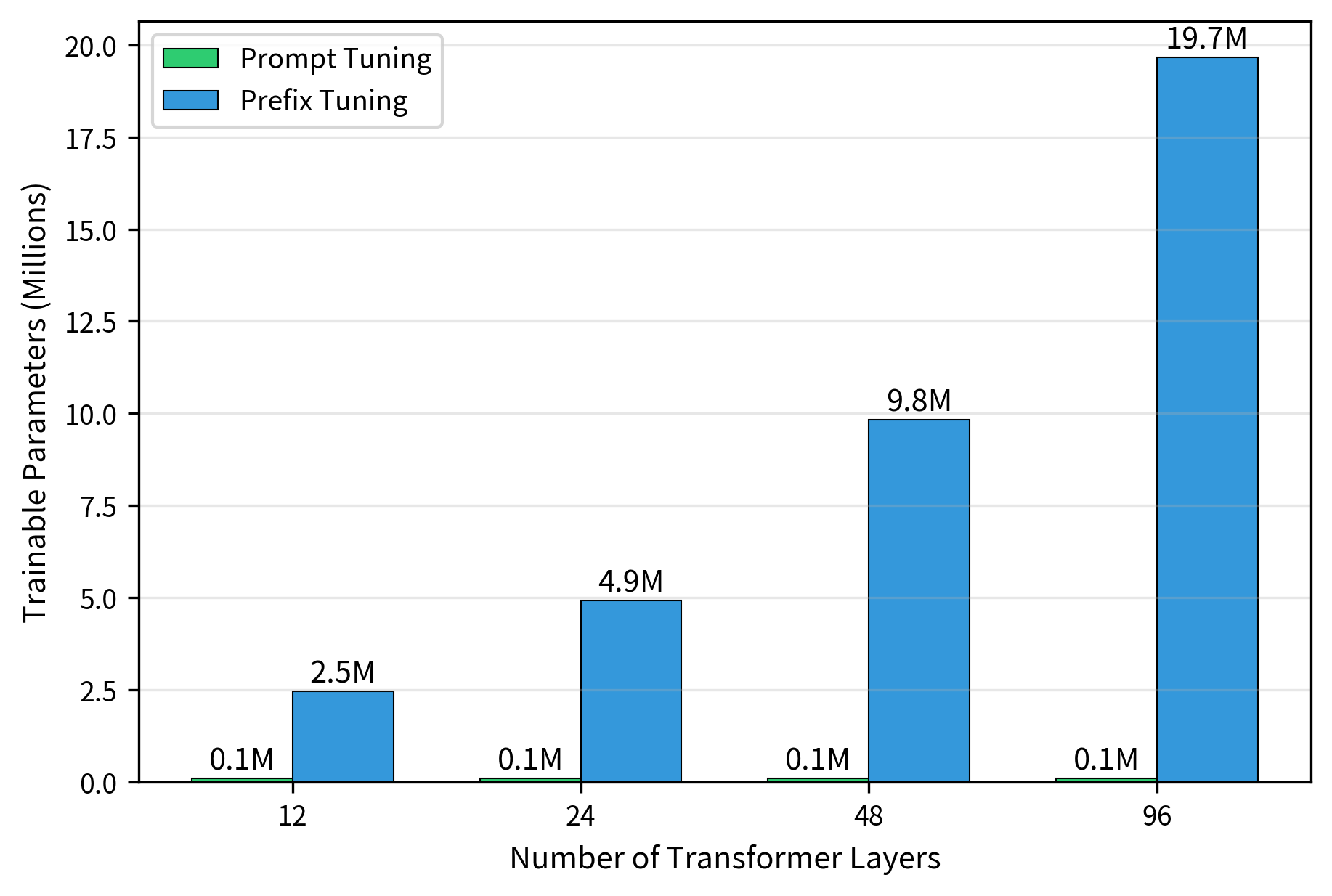
This design choice has several implications. First, the parameter count becomes independent of model depth. A 12-layer or 96-layer model requires the same parameters, determined only by prompt length and embedding dimension. Second, the approach is architecturally simpler because there are no modifications to any transformer layer. The soft prompts are simply concatenated with the embedded input and processed normally.

The key insight driving prompt tuning is that large language models have learned such rich internal representations that a small modification at the input level can cascade through the network to produce task-appropriate outputs. The success of this approach depends critically on model scale, as we will see when examining the scaling behavior later in this chapter.

To understand prompt tuning mathematically, let's examine how soft prompts integrate with the standard transformer input pipeline. In a typical transformer model, input text first passes through tokenization, then each token is mapped to a dense vector through the embedding layer. Prompt tuning intervenes at this point by inserting learnable vectors. The frozen model treats these as embeddings of additional tokens.

Let $\mathbf{X} \in \mathbb{R}^{n \times d}$ represent the embedded input sequence, where $n$ is the sequence length and $d$ is the embedding dimension. This matrix contains one row for each input token, with each row being a $d$-dimensional vector that encodes both the token's meaning and its position in the sequence. Prompt tuning introduces a trainable prompt matrix $\mathbf{P} \in \mathbb{R}^{p \times d}$, where $p$ is the prompt length. Each row of this matrix represents one learnable "virtual token" that exists purely in the continuous embedding space.

We form the augmented input by prepending the soft prompt matrix to the original input sequence:

where:

• $\mathbf{X}'$: the augmented input matrix containing both prompt and data
• $\mathbf{P}$: the matrix of learnable soft prompt parameters
• $\mathbf{X}$: the original input embedding matrix
• $[\cdot; \cdot]$: the concatenation operation along the sequence length dimension

The concatenation operation stacks the prompt matrix on top of the input matrix, creating a new sequence that begins with $p$ soft prompt tokens followed by the $n$ actual input tokens. From your transformer's perspective, this augmented sequence looks just like any other embedded input, except that the first $p$ positions contain learned vectors rather than embeddings looked up from the vocabulary. This is key to prompt tuning's simplicity: no architectural modifications are needed.

This concatenated sequence is then processed by the frozen transformer normally. The frozen model applies its full sequence of attention layers and feed-forward networks without any awareness that the first few tokens are special. If we denote the frozen language model as $f_\theta$, the output is computed as:

where:

• $\mathbf{Y}$: the output representations from the transformer
• $f_\theta$: the frozen transformer function parameterized by weights $\theta$
• $[\mathbf{P}; \mathbf{X}]$: the concatenated sequence of prompt and input embeddings

During training, only $\mathbf{P}$ receives gradient updates. The entire transformer with parameters $\theta$ remains frozen, meaning that backpropagation computes gradients for the prompt parameters but treats the model weights as constants. The training objective is the standard task loss, whether cross-entropy for classification, language modeling loss for generation, or any other task-appropriate objective. The gradients flow backward through the frozen model, ultimately reaching and updating only the soft prompt embeddings.

Prompt tuning's simplicity is most evident when we examine its parameter count. Since soft prompts exist only at the input level, trainable parameters depend solely on the number of virtual tokens and embedding dimension. The number of trainable parameters in prompt tuning is:

where:

• N_params: the total number of trainable parameters
• $p$: the length of the soft prompt (number of virtual tokens)
• $d$: the embedding dimension of the model

To make this concrete, consider a model with embedding dimension $d = 1024$ and prompt length $p = 100$. This configuration yields exactly 102,400 parameters, approximately 0.01% of a 1 billion parameter model. This is a dramatic reduction compared to full fine-tuning, where all billion parameters receive gradient updates.

The comparison with prefix tuning is equally striking. Prefix tuning requires parameters proportional to $p \times L \times 2d$, where $L$ is the number of layers and the factor of 2 accounts for both keys and values at each layer. For a 24-layer model with the same embedding dimension and prompt length, prefix tuning would require 48 times more parameters than prompt tuning. Prompt tuning's parameter count remains constant regardless of model depth, making it more attractive as models grow deeper.

The formulation reveals a key difference from prefix tuning that has important implications for how each method steers the model's behavior. In prefix tuning, the soft prefixes directly modify the attention computation at every layer by adding to the keys and values:

where:

• $\mathbf{Q}$: the query matrix derived from the current layer's input
• $\mathbf{P}_K, \mathbf{P}_V$: the trainable prefix matrices for keys and values
• $\mathbf{K}, \mathbf{V}$: the key and value matrices derived from the input
• $[\cdot; \cdot]$: the concatenation operation extending the keys and values

This direct injection means that every attention head at every layer has access to learned key-value pairs that can guide its computations. The prefixes effectively provide "steering information" directly where the model makes attention decisions. In contrast, soft prompts in prompt tuning only appear as additional "tokens" in the input sequence. They do not directly modify any attention matrices or feed-forward computations. Instead, the model's own attention mechanism decides how much to attend to these soft prompts versus the actual input tokens at each layer. This represents a more indirect form of intervention because prompt tuning relies on the model learning to use soft prompts through its natural attention patterns rather than injecting information directly into the attention computation. The soft prompts must earn their influence by being useful for the task, as determined by the attention weights the model computes.

This architectural difference explains why prompt tuning requires larger model scale to match prefix tuning's performance. Smaller models lack the capacity to propagate task-relevant information from input soft prompts through many layers. Each layer's computations dilute and transform the representations. Smaller models with fewer parameters per layer struggle to preserve task-specific signals across this deep processing. Larger models, by contrast, have richer internal representations and more parameters to capture subtle patterns, allowing them to more effectively leverage input-level modifications by learning attention patterns that extract and preserve relevant information from soft prompts.

How should you initialize the soft prompt matrix $\mathbf{P}$? This practical question directly affects whether your training succeeds. Unlike weight matrices in neural networks, where random initialization with appropriate scaling typically works well, prompt initialization significantly impacts prompt tuning performance, especially for smaller models. The reason is rooted in the embedding space. Transformers are trained to process vocabulary token embeddings, a specific vector distribution. Soft prompts that start far from this distribution may create representations that the model struggles to interpret meaningfully. Several strategies have been explored to address this challenge.

The simplest approach initializes each prompt embedding from a random distribution:

where:

• $\mathbf{P}_{ij}$: the element at index $(i,j)$ of the prompt matrix
• $\mathcal{U}(-a, a)$: a uniform distribution bounded by $a$
• $\mathcal{N}(0, \sigma^2)$: a normal distribution with mean $0$ and variance $\sigma^2$

The hyperparameters $a$ or $\sigma$ are typically chosen to match the model's existing embedding scale, often determined empirically or set to small values like 0.02. Random initialization provides no task-related inductive bias. The optimization process must discover useful prompt embeddings entirely from the training signal, starting from a point that may lie outside the manifold of meaningful token representations. This approach works reasonably well for large models with sufficient capacity to correct for poor starting points, but it can lead to suboptimal results if you're working with smaller models or when you have limited training data.

A more informed strategy initializes prompt embeddings using existing token embeddings from the model's vocabulary. The intuition is straightforward: the frozen model has learned to process vocabulary embeddings effectively during pretraining. By starting in the same region of embedding space, you give the soft prompts a head start. For each prompt position $i$, you sample a random token $t_i$ from the vocabulary and use its embedding:

where:

• $\mathbf{P}_i$: the initialization vector for the $i$-th prompt token
• $\mathbf{E}$: the model's embedding matrix
• $t_i$: the index of the sampled vocabulary token

This ensures soft prompts start in embedding space the model already processes meaningfully. Since attention mechanisms are designed to work with vectors from this distribution, starting nearby may accelerate optimization. During training, the prompts can then drift away from their initial positions to better serve your task, but they begin in territory the model understands. The particular tokens you choose for initialization matter less than the fact that we are sampling from the correct distribution.

For classification tasks, you can enhance vocabulary initialization by selecting tokens related to task or class labels. For sentiment classification, you might initialize using the embeddings of tokens like "positive", "negative", "sentiment", "review":

where:

• $\mathbf{P}_i$: the initialization vector for the $i$-th prompt token
• $\mathbf{E}$: the pretrained embedding matrix
• $\text{class\_token}_i$: the token index corresponding to a class label or task-relevant word

This provides a strong inductive bias, giving the optimizer a starting point that already encodes task-relevant semantics. The training process then refines these embeddings to better capture the specific classification boundary. In effect, you're telling the model to "start by thinking about these concepts" and letting gradient descent figure out exactly how to think about them. For tasks where the class labels have clear lexical representations, this initialization can significantly reduce the number of training steps required to achieve good performance.

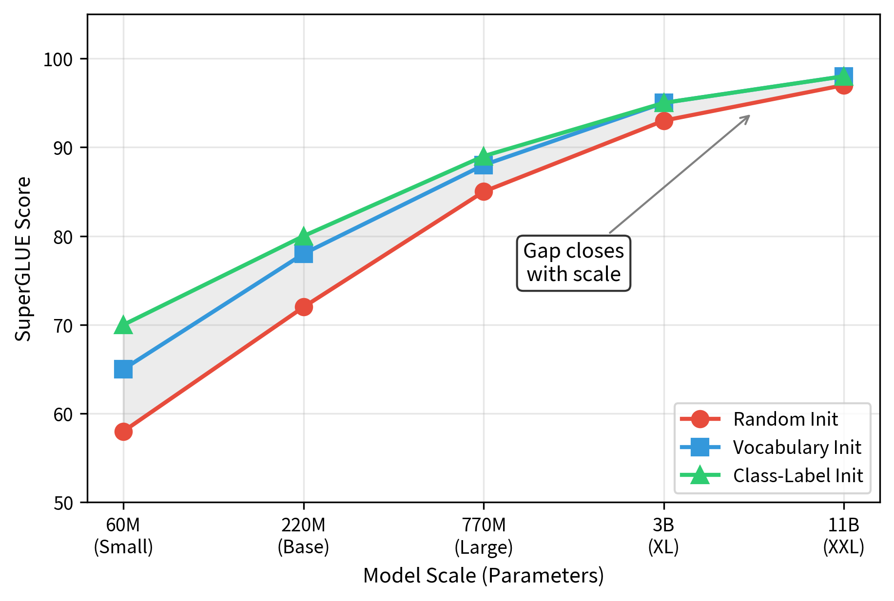
The original prompt tuning paper by Lester et al. found that initialization strategy matters most at smaller model scales. For T5-Small (60 million parameters), class-label initialization significantly outperformed random initialization by several percentage points on benchmark tasks. The gap was substantial enough to change conclusions about whether prompt tuning was viable for smaller models. As model scale increased to T5-XXL with 11 billion parameters, the gap closed and all strategies converged to similar final performance. This convergence suggests that larger models are more robust to initialization choices.

This pattern shows that larger models can recover from poor initialization during training, while smaller models with limited capacity benefit from starting closer to a good solution. Smaller models have more challenging optimization landscapes where poor initialization leads to suboptimal local minima. In practice, vocabulary or class-label initialization adds minimal implementation complexity and provides a safety margin against poor convergence, making vocabulary or class-label initialization the recommended default regardless of model scale.

The most compelling finding from the prompt tuning research is its scaling behavior. This sets prompt tuning apart from many parameter-efficient methods that trade performance for efficiency at any scale. As model scale increases, prompt tuning's performance gap with full fine-tuning shrinks until they achieve equivalent performance.

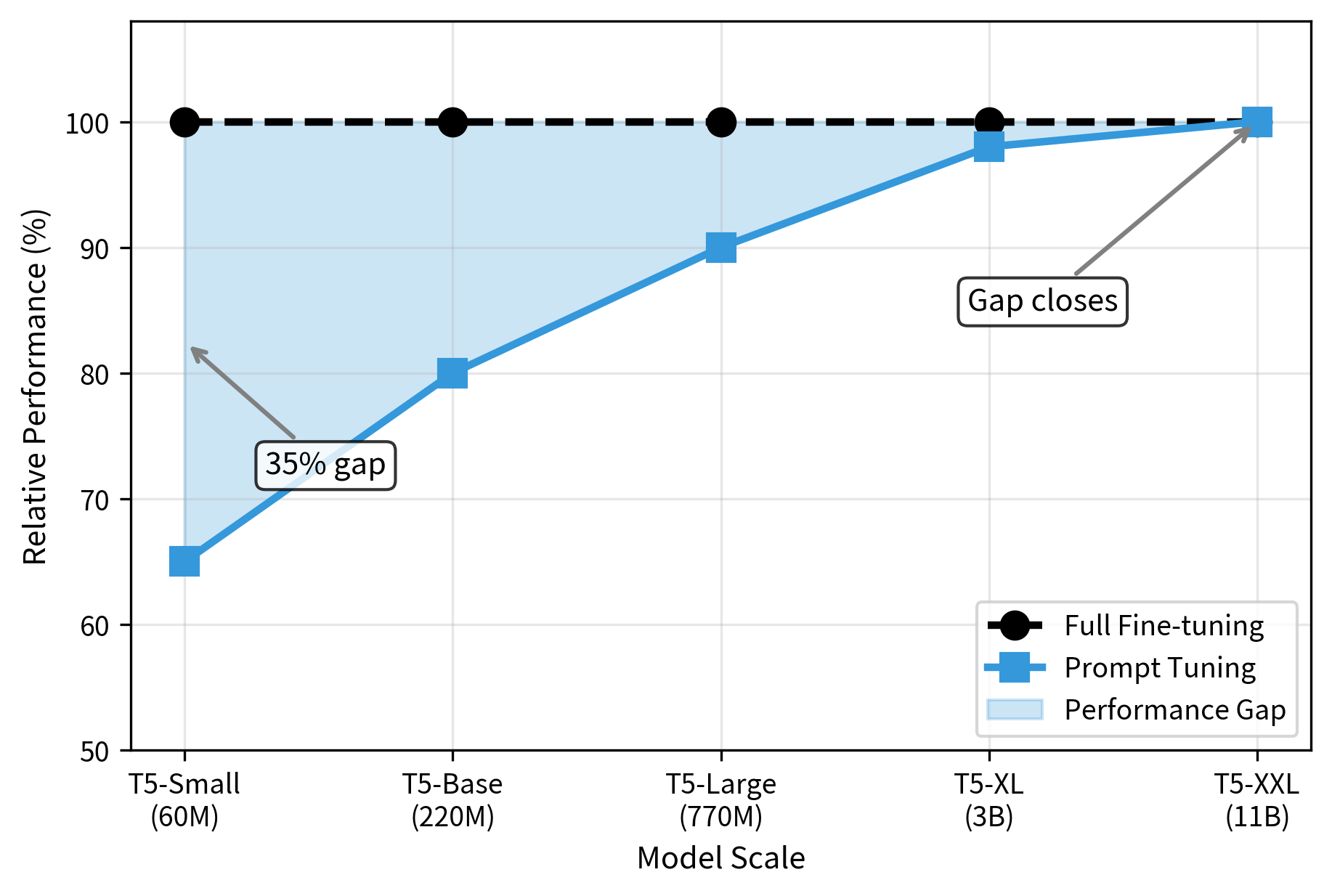
Lester et al. evaluated prompt tuning across the T5 model family on the SuperGLUE benchmark, a challenging suite of natural language understanding tasks. The results showed a clear and consistent trend that held across multiple tasks. At T5-Small (60M parameters), prompt tuning achieves only 65% of full fine-tuning performance, a gap that makes prompt tuning impractical at this scale. This gap motivated research into how to improve prompt tuning's effectiveness. For T5-Base with 220 million parameters, this improved to around 80%, a meaningful improvement but still a notable gap. By T5-Large with 770 million parameters, the gap narrowed further to about 90%, entering territory where prompt tuning became a viable option for many applications. At T5-XL (3B) and T5-XXL (11B), prompt tuning matches full fine-tuning performance, eliminating any efficiency penalty.

This scaling behavior can be understood through the lens of model capacity and representational richness. Smaller models have limited representational power distributed across their layers. When only the input embeddings are modified, the model has limited flexibility to adapt its behavior for a new task. The internal computations are constrained by the model's size, and the soft prompt signal may be diluted or lost as it propagates through the network. Larger models, with richer internal representations and more expressive attention patterns, can more flexibly adapt their computations based on the soft prompt context. They have enough parameters at each layer to learn how to extract and use the task-specific information encoded in the soft prompts.

This scaling behavior has important implications for when to use prompt tuning. For very large models with billions of parameters, prompt tuning offers comparable performance to full fine-tuning while training orders of magnitude fewer parameters. This makes many adaptation scenarios practical that would be impossible with full fine-tuning due to memory constraints. A 10B model typically requires hundreds of gigabytes of GPU memory for full fine-tuning, but prompt tuning needs only enough for gradients of ~100K parameters.

However, smaller models often show larger performance gaps that may disqualify prompt tuning for accuracy-critical applications. If you're adapting a 100 million parameter model, prompt tuning alone might not achieve acceptable performance for your use case. For these situations, consider prefix tuning (which intervenes at every layer) or LoRA (which modifies weight matrices through low-rank updates). An upcoming chapter compares PEFT methods systematically to guide your choices.

Several hypotheses explain why larger models benefit more from prompt tuning. Understanding these helps determine when prompt tuning will - Larger models have more attention heads, allowing different heads to specialize in attending to soft prompts versus input tokens. Some heads learn to extract task instructions from the soft prompts while others focus on processing the input, enabling a division of labor that smaller models cannot achieve.

• Larger models have more layers, providing more opportunities for the soft prompt information to be integrated and refined. Each layer progressively transforms the representations to make the task-relevant signal clearer.
• Larger models have learned richer representations during pretraining that can more flexibly recombine based on context. Their embedding spaces capture finer distinctions between concepts, making it easier for small modifications to trigger appropriate behaviors.

Prompt tuning resembles in-context learning (discussed earlier) because it learns an optimal 'soft context' that activates the model's task-solving capabilities. Soft prompts function as compressed instructions that define the task, similar to how few-shot examples work. Larger models, which exhibit stronger in-context learning abilities with discrete prompts, can more effectively leverage this learned continuous context. The properties that make large models effective at following natural language instructions also help them follow learned soft prompt instructions.

The prompt length $p$ is the primary hyperparameter in prompt tuning, and understanding its effects is crucial for achieving good results. Longer prompts provide more learnable parameters to encode task-specific information. However, longer prompts also consume more of the model's context window, leaving less room for actual input tokens. Finding the right balance means understanding how prompt length interacts with task complexity, model capacity, and practical constraints.

Empirical studies show that performance improves with prompt length initially, then plateaus or declines. Early tokens provide substantial benefit, while additional tokens show diminishing returns. The optimal length depends on the task and model:

• Very short prompts (1-5 tokens): Often lack capacity to encode task requirements, resulting in underperformance. A single token may not have enough dimensions to capture the nuances of a classification task.
• Short prompts (10-20 tokens): Can work well for simple tasks like binary classification where the model needs to know it's handling a sentiment task or similar basic instruction.
• Medium prompts (20-100 tokens): The sweet spot for most tasks, balancing expressiveness with efficiency. This range provides enough capacity for complex task definitions while maintaining manageable parameter counts. Good performance can be achieved without excessive computational overhead.
• Long prompts (100+ tokens): Diminishing returns; additional parameters don't translate to better performance and may harm performance through optimization difficulties or by encouraging overreliance on soft prompts instead of input.

More complex tasks generally benefit from longer prompts, though the relationship depends on the nature of the task's complexity. For simple sentiment classification with two clear categories, you might use a 20-token prompt to encode the task definition. For complex reasoning tasks or multi-class classification with many categories, you should consider prompts of 50-100 tokens to capture necessary nuances.

The intuition is clear: soft prompts must encode both the task definition (expected outputs) and task-specific patterns (relevant input features). More complex tasks require more "virtual instructions" encoded in the prompt embeddings. A sentiment classifier needs only to encode "map positive language to class 1 and negative language to class 0," while a topic classifier with 20 categories must represent all distinctions in the soft prompt representations.

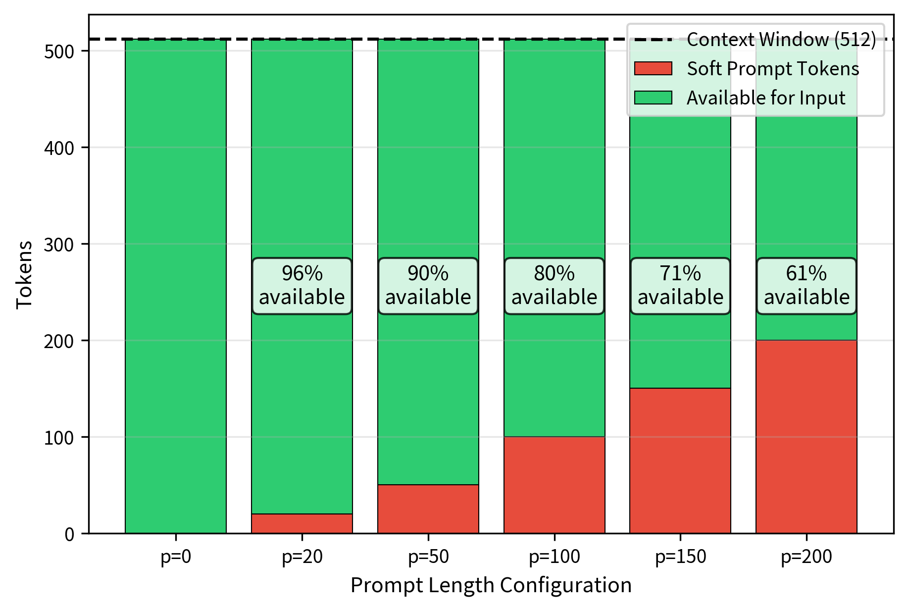
A practical consideration is the context window trade-off. If a model has a 512 token context window and uses a 100 token prompt, only 412 tokens remain for the actual input. For tasks with long documents, this may force truncation of important content, potentially harming performance more than the longer prompt helps.

This trade-off is more acute for prompt tuning than prefix tuning. Prefix tuning adds key-value pairs to the attention computation rather than the sequence, so they don't consume input token space. Prompt tuning's soft prompts are true virtual tokens that compete with input tokens for the attention window. When designing a prompt tuning solution, you should consider typical input length and ensure the prompt doesn't consume so much context that important input is lost. For applications with highly variable input lengths, this may require prompt lengths that work well across the distribution rather than optimizing for average-length inputs.

Let's implement prompt tuning for a text classification task to see how it works in practice. We'll create a prompt-tunable wrapper around a frozen transformer model.

The core of prompt tuning is a learnable embedding matrix that gets prepended to the input. We create a module that handles the soft prompt generation and concatenation.

Now we'll create a complete classifier that combines the soft prompts with a frozen pretrained model.

Let's instantiate the model and examine the parameter efficiency.

With just 20 soft prompt tokens, the model updates approximately 0.02% of the total parameters. The soft prompt embeddings contribute $20 \times 768 = 15,360$ parameters (mostly from the soft prompts), and the classification head adds $768 \times 2 + 2 = 1,538$ parameters.

Let's create a simple training example to demonstrate how prompt tuning works in practice.

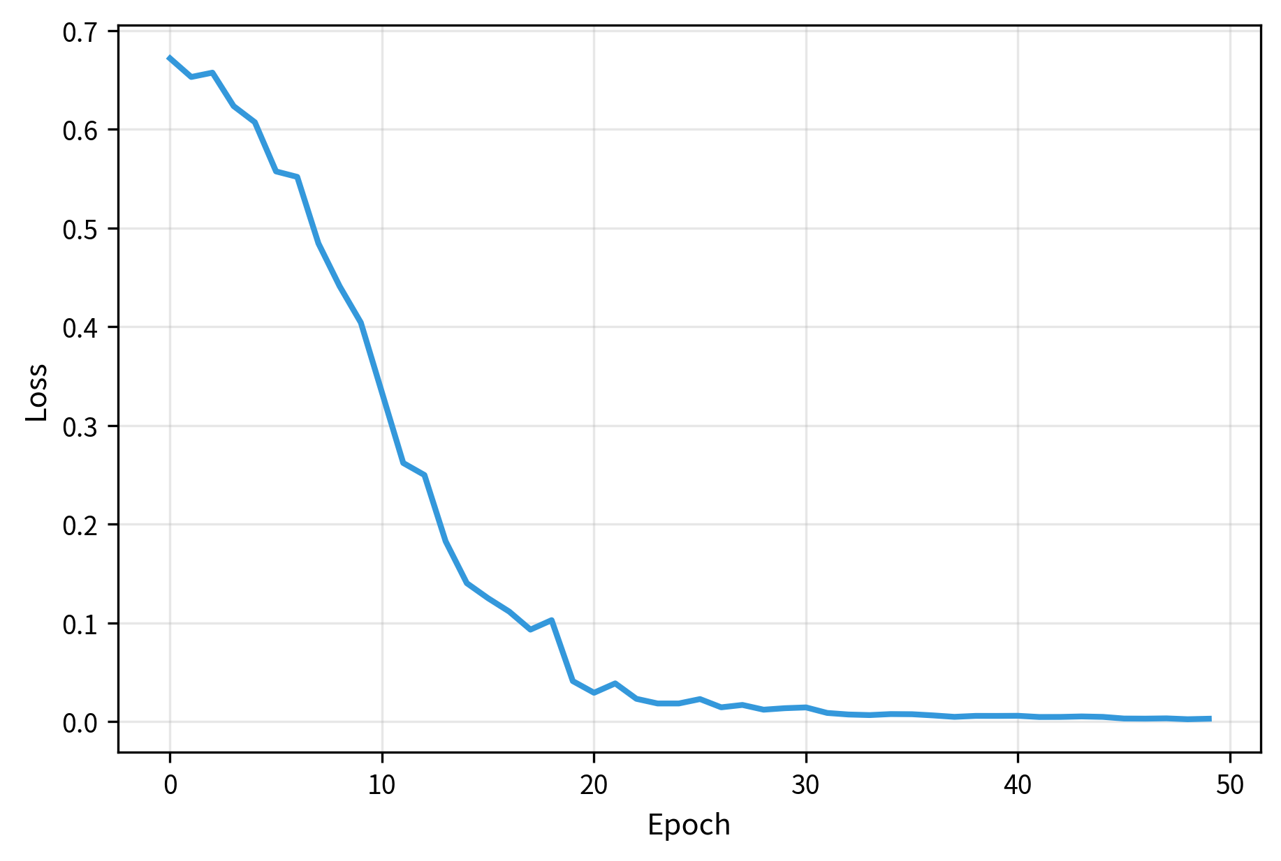
The training loss decreases smoothly, demonstrating that the model can learn the classification task by updating only the soft prompt embeddings. Despite training just 0.02% of parameters, the model successfully adapts to the sentiment classification task.

The model correctly classifies the test examples, identifying positive and negative sentiments accurately. This demonstrates that the small set of trainable soft prompt parameters is sufficient to steer the frozen model's behavior for this task.

Let's compare random versus vocabulary initialization to see the effect on early training dynamics.

The vocabulary-initialized model often shows slightly faster initial convergence, though both approaches eventually reach similar performance. This difference becomes more pronounced with smaller models or limited training data.

One interesting property of prompt tuning is that we can analyze the learned soft prompts to understand what the model has learned.

The nearest vocabulary tokens to each soft prompt provide insight into what semantic concepts the model has encoded. For a sentiment classification task, we might expect to see tokens related to sentiment, evaluation, or opinion.

Let's empirically examine how prompt length affects model performance by training models with different prompt lengths.

The results demonstrate the trade-off with prompt length. Very short prompts may lack the capacity to encode task requirements, while very long prompts provide diminishing returns and may even slightly hurt performance due to optimization challenges. The sweet spot typically lies in the 10-50 token range for most classification tasks.

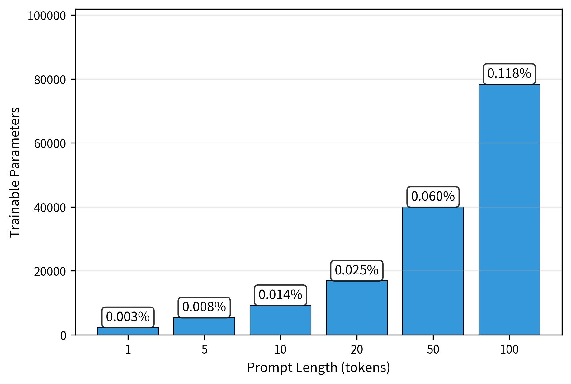
Even with 100 prompt tokens, we're training less than 0.12% of the model's parameters. This extreme parameter efficiency is what makes prompt tuning attractive for scenarios with limited compute or when maintaining many task-specific adaptations.

Key parameters:

• num_prompt_tokens: Number of soft prompt tokens prepended to the input
• init_from_vocab: Whether to initialize prompts from the model's vocabulary
• embedding_dim: Dimension of the prompt embeddings (must match model)

Prompt tuning represented a significant advance in parameter-efficient fine-tuning, demonstrating that remarkably few parameters could adapt large models to new tasks. However, understanding its limitations is crucial for effective use. The most significant limitation is the scale dependence discussed earlier. While prompt tuning matches full fine-tuning at 10B+ parameter scales, smaller models exhibit a meaningful performance gap. This creates a practical challenge. Large models benefit most from prompt tuning, while smaller models may benefit more from alternatives such as LoRA or prefix tuning that directly modify model computation. This scale requirement partially offsets the democratization benefits of parameter-efficient methods. A second limitation involves the interpretability of learned prompts. Unlike discrete prompts, which are human-readable, soft prompts exist only in embedding space. Finding nearest vocabulary neighbors provides only rough insight into the learned representations. For applications requiring transparency or auditing of the adaptation mechanism, soft prompts present challenges that discrete prompting avoids.

The context window trade-off deserves consideration. Every soft prompt token consumes one position in the model's context window, which can be significant for tasks involving long documents or conversations. A 100-token soft prompt in a 512-token context model leaves only 412 tokens for actual input, potentially forcing truncation of important content. Prefix tuning, while requiring more parameters, does not consume input tokens' context space in the same way.

Despite these limitations, prompt tuning's impact on the field has been substantial. It demonstrated the power of scale for parameter-efficient methods, showing that simpler approaches can match complex ones given sufficient model capacity. This finding influenced subsequent research into understanding why large models are so adaptable and how to leverage this adaptability efficiently. The simplicity of prompt tuning also made it accessible: unlike methods requiring modifications to transformer architectures, prompt tuning works with any model that accepts embedding inputs.

Prompt tuning also became an important benchmark for comparing PEFT methods. The scaling curves from the original paper became a reference point, with subsequent methods often demonstrating their value by showing better performance than prompt tuning at smaller scales while maintaining efficiency at larger scales.

Prompt tuning simplifies parameter-efficient fine-tuning by prepending learnable soft prompt embeddings to the input. Unlike prefix tuning, which modifies attention computations at every layer, prompt tuning operates only at the input level, trusting the frozen model to propagate task-relevant information through its layers.

Key concepts:

• Formulation: Soft prompts $\mathbf{P} \in \mathbb{R}^{p \times d}$ are concatenated with input embeddings and processed by the frozen model normally, with only $\mathbf{P}$ receiving gradient updates during training.

• Initialization strategies: Vocabulary initialization uses existing token embeddings as starting points and generally outperforms random initialization, especially for smaller models. Class-label initialization provides even stronger inductive bias for classification tasks.

• Scaling behavior: The performance gap between prompt tuning and full fine-tuning shrinks as model scale increases. At 10B+ parameters, prompt tuning matches full fine-tuning, making it increasingly attractive for very large models.

• Prompt length effects: Moderate prompt lengths (10-100 tokens) typically work best. Very short prompts lack capacity while very long prompts provide diminishing returns and consume context window space.

The parameter efficiency of prompt tuning is remarkable: adapting a 10B parameter model might require training only 0.01% of parameters. This enables you to maintain hundreds of task-specific adaptations for a single base model, dramatically reducing storage and deployment costs.

The next chapter explores adapter layers, a different approach that inserts small trainable modules between transformer layers, providing an alternative intervention point for efficient adaptation. Subsequent chapters compare all PEFT methods systematically to help you choose when to use each approach.

Ready to test your understanding? Take this quick quiz to reinforce what you've learned about prompt tuning and its parameter-efficient approach to model adaptation.