

Master autoregressive and moving average models for financial time-series. Learn stationarity, ACF/PACF diagnostics, ARIMA estimation, and forecasting.
Choose your expertise level to adjust how many terms are explained. Beginners see more tooltips, experts see fewer to maintain reading flow. Hover over underlined terms for instant definitions.
Time-Series Models for Financial Data
Financial markets generate vast streams of sequential observations: prices, returns, interest rates, volatility measures, and economic indicators. Understanding the temporal structure of these data is essential for forecasting, risk management, and trading strategy development. Time-series models provide a principled framework for capturing the statistical dependencies that exist between observations across time.
Unlike the stochastic differential equations we explored in earlier chapters on Brownian motion and Itô calculus, the models in this chapter operate in discrete time and focus on the autocorrelation structure of observed data. While Black-Scholes assumes returns are independent and identically distributed, empirical evidence from our study of stylized facts reveals that financial returns exhibit serial correlation in their magnitudes (volatility clustering) and occasional predictable patterns in their levels. Time-series models give us the tools to detect, quantify, and exploit these patterns.
This chapter introduces the foundational autoregressive (AR) and moving average (MA) models, then combines them into the ARMA framework for stationary series. We extend to ARIMA models for handling non-stationary data like trending economic indicators or asset prices. Throughout, we develop practical skills for model identification using autocorrelation analysis, parameter estimation, and forecasting with proper uncertainty quantification.
Stationarity: The Foundation of Time-Series Analysis
Before building any time-series model, we must understand stationarity, a property that determines which modeling techniques apply and whether our statistical estimates are meaningful. The concept of stationarity addresses a fundamental challenge in time-series analysis: how can we learn about a process when we observe only a single realization of it? If the statistical properties of a series change arbitrarily over time, then observations from the past tell us nothing reliable about the future. Stationarity provides the stability assumption that makes statistical inference possible.
Think of stationarity as a form of temporal homogeneity. Just as we assume in cross-sectional statistics that observations come from the same underlying distribution, stationarity assumes that the time series comes from a process whose statistical character remains consistent across time. This does not mean the series is constant or predictable. Rather, it means the rules governing its behavior do not change.
Strict and Weak Stationarity
A time series is strictly stationary if its joint probability distribution is invariant to time shifts. For any set of time indices and any shift , the joint distribution of equals that of . This is a strong requirement rarely verified in practice. Strict stationarity essentially demands that if you were to examine any collection of observations from the series, you could not tell what time period they came from based solely on their statistical properties. The distribution of Monday's return and the following Wednesday's return must be identical to the distribution of any other Monday-Wednesday pair, regardless of when those observations occur.
More useful is weak stationarity (or covariance stationarity), which requires only:\n\n1. Constant mean: for all 2. Constant variance: for all 3. Autocovariance depends only on lag: for all
Weak stationarity relaxes the strict requirement by focusing only on the first two moments of the distribution. We do not require the entire distribution to be time-invariant, only the mean, variance, and the covariance structure. This makes weak stationarity much easier to test and work with in practice. The third condition is particularly important: it states that the covariance between observations depends only on how far apart they are in time (the lag ), not on their absolute position in the series. The covariance between observations 5 periods apart must be the same whether we are looking at periods 1 and 6 or periods 100 and 105.
The autocovariance function measures how observations separated by periods covary. This function captures the memory of the process, telling us how much information about the current value is contained in values from periods ago. The autocorrelation function (ACF) normalizes this to a scale that is easier to interpret:
where:
- : value of the series at time
- : autocorrelation at lag
- : autocovariance at lag
- : variance of the series ()
- : covariance between observations periods apart
The normalization by (the variance) ensures that autocorrelations are bounded between -1 and 1, just like ordinary correlation coefficients. For a stationary series, always holds because any observation is perfectly correlated with itself. The constraint for all lags follows from the Cauchy-Schwarz inequality. The ACF provides a complete summary of the linear dependence structure of a stationary time series and serves as our primary diagnostic tool for model identification.
Stationarity in Financial Data
Asset prices are almost never stationary: they exhibit trends, drift, and variance that changes over time. The S&P 500 today is systematically higher than it was 50 years ago, violating the constant mean requirement. This non-stationarity is not a modeling failure but reflects genuine economic reality. Over long horizons, stock prices tend to rise because companies generate earnings and reinvest profits, creating compound growth in value. A statistical model that assumed stock prices fluctuate around a fixed mean would fundamentally mischaracterize how equity markets work.
However, returns are often approximately stationary:
where:
- : return at time
- : price at time
- : price at time
The transformation from prices to returns removes the trending behavior. Log returns fluctuate around a relatively stable mean (often close to zero for daily data) with variance that, while exhibiting clustering, maintains a long-run average. Intuitively, while the price level can wander arbitrarily far from any fixed reference point, the percentage changes in price tend to stay within a bounded range. This is why most time-series modeling in finance focuses on returns rather than prices. The transformation to returns is not just a mathematical convenience; it reflects the economic intuition that investors care about percentage gains and losses, not absolute price levels.
A series is integrated of order , written , if it must be differenced times to achieve stationarity. Asset prices are typically : one difference (the return) yields a stationary series. Economic series like GDP may be or .
Autoregressive (AR) Models
Autoregressive models capture the idea that today's value depends linearly on past values. This concept reflects a fundamental intuition about how many processes evolve: the current state of a system depends on where it was recently. An AR(p) model expresses the current observation as a weighted sum of the previous observations plus a noise term. The term "autoregressive" means the series is regressed on its own past values, unlike ordinary regression which uses external variables.
The AR(1) Model
To capture the linear dependence of the current observation on its immediate predecessor, the simplest autoregressive model is AR(1). This model embodies the idea that today's value is pulled toward its previous value, with some random perturbation added. Mathematically:
where:
- : value of the series at time
- : value of the series at time
- : constant (intercept)
- : autoregressive coefficient
- : white noise term with mean 0 and variance
The white noise terms are assumed independent: for . This independence assumption is crucial because it means all the predictable structure in the series comes from the autoregressive relationship, not from patterns in the shocks themselves. The parameter controls the strength and direction of persistence. When is positive, high values tend to be followed by high values and low values by low values. When is negative, the series tends to oscillate, with high values followed by low values and vice versa. The magnitude of determines how strong this tendency is.
Stationarity Conditions
For AR(1) to be stationary, we require . This condition ensures that the influence of past shocks decays over time rather than persisting indefinitely or exploding. To see why this condition is necessary, assume stationarity holds and take expectations of both sides of the AR(1) equation:
where:
- : expectation operator
- : value of the series at time
- : constant term
- : autoregressive coefficient
- : white noise term
Since under stationarity (the mean must be the same at all time periods), and by the white noise assumption, we can solve for the unconditional mean:
where:
- : mean of the process
- : constant term
- : autoregressive coefficient
This solution exists only if . If , the denominator becomes zero and no finite mean exists, indicating a non-stationary process known as a random walk. Moreover, computing the variance requires using the independence of and . This independence follows from the assumption that is unpredictable given past information:
where:
- : variance at time
- : constant term
- : autoregressive coefficient
- : white noise term
- : variance of the white noise term
Under stationarity with , we can substitute and solve for the unconditional variance:
where:
- : variance of the process ()
- : variance of the white noise term
- : autoregressive coefficient
This expression is positive and finite only if , meaning . When , the variance formula would yield either a negative number (impossible) or infinity (the series explodes). The stationarity condition thus emerges naturally from requiring that both the mean and variance be well-defined finite constants.
ACF of AR(1)
The autocorrelation function of AR(1) decays geometrically, a signature pattern that helps us identify AR processes in empirical data. To derive the autocovariance, we work with the mean-centered series to simplify calculations. The deviation from the mean satisfies . Multiplying both sides by for and taking expectations yields the autocovariance at lag :
where:
- : autocovariance at lag
- : expectation operator
- : value of the series at time
- : mean of the process
- : autoregressive coefficient
- : white noise term
- : autocovariance at lag
The key insight is that for because the current shock is uncorrelated with past values of the series. This recursion yields by repeated substitution, so the autocorrelation function has an elegant closed form:
where:
- : autocorrelation at lag
- : autoregressive coefficient
- : lag number
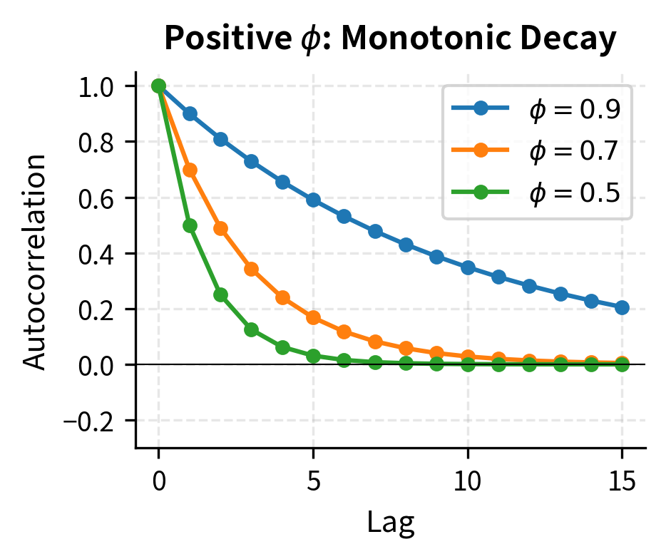
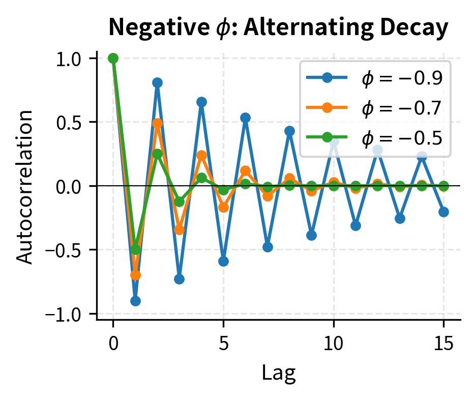
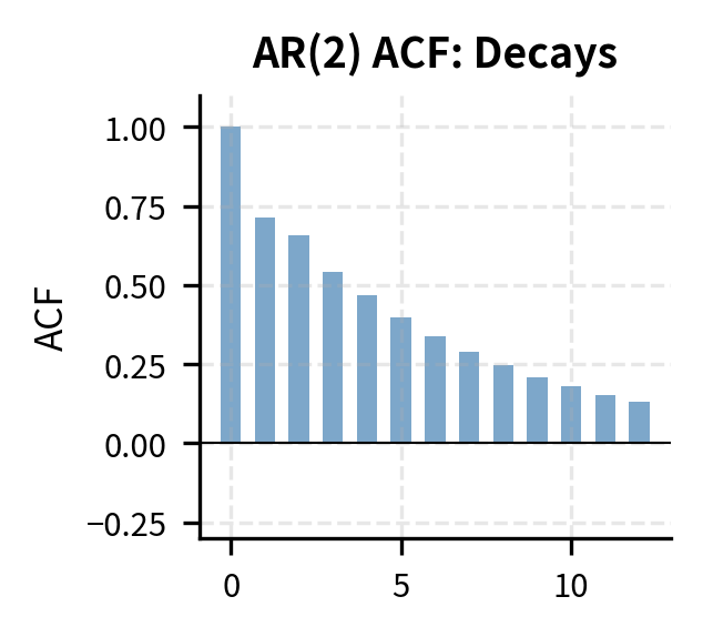
When , correlations decay exponentially but remain positive at all lags. This positive persistence means high values tend to be followed by somewhat high values, with the memory gradually fading. When , correlations alternate in sign while decaying in magnitude. This creates an oscillating pattern where high values tend to be followed by low values, then moderately high values, and so on. The geometric decay pattern is the hallmark of AR(1) and provides a clear diagnostic signature in sample ACF plots.
General AR(p) Models
The AR(p) model extends the first-order case to include lags, allowing for more complex dependence structures where observations depend on multiple past values:
where:
- : value of the series at time
- : constant term
- : autoregressive coefficient at lag
- : white noise error term
The multiple lags can capture more nuanced dynamics. For instance, an AR(2) model might exhibit cyclical behavior if the coefficients are chosen appropriately, which a simple AR(1) cannot produce. Using the lag operator where , we can express the AR(p) model compactly:
where:
- : value of the series at time
- : lag operator such that
- : autoregressive coefficient at lag
- : constant term
- : white noise error term
We write this as where is called the autoregressive polynomial. The lag operator notation provides not just compactness but also mathematical power, allowing us to manipulate time-series equations using algebraic techniques.
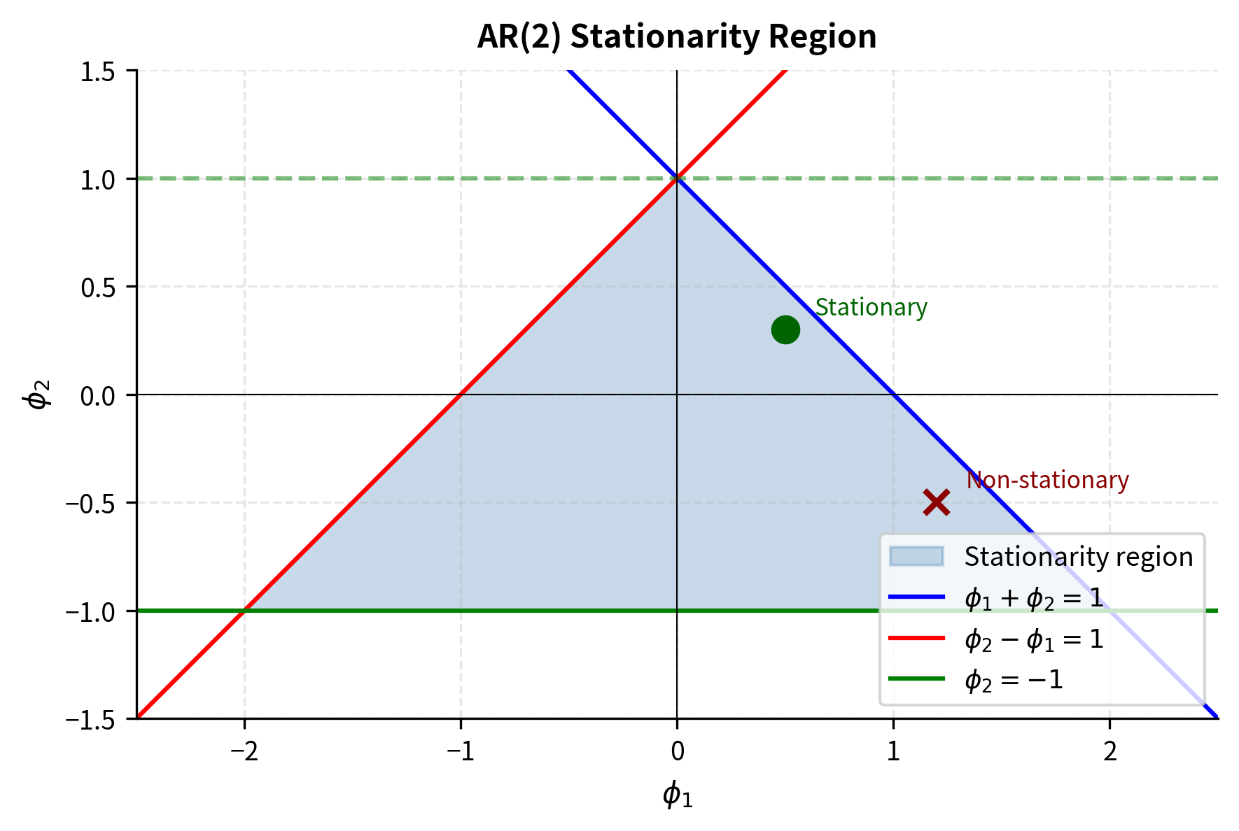
Stationarity requires all roots of the characteristic polynomial to lie outside the unit circle in the complex plane. This generalizes the AR(1) condition to higher-order models. For AR(2) with , the stationarity conditions can be expressed as three inequalities:
where:
- : autoregressive coefficients of the AR(2) model
These conditions define a triangular region in the parameter space where stationary AR(2) processes exist. Outside this region, the process either explodes or exhibits non-stationary wandering behavior.
Partial Autocorrelation Function (PACF)
The partial autocorrelation at lag , denoted , measures the correlation between and after removing the linear effects of intermediate lags . This "partial" correlation isolates the direct relationship between observations periods apart, controlling for everything in between. The intuition is similar to partial correlation in regression analysis: we want to know how much additional information provides about beyond what is already captured by the intervening observations.
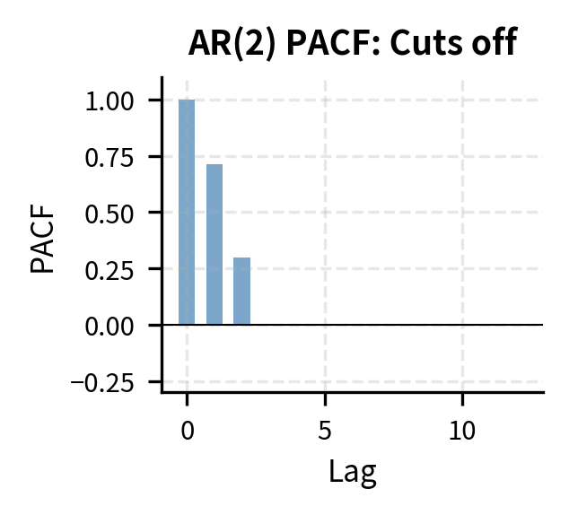
For an AR(p) process, a key identification property holds:
where:
- : partial autocorrelation at lag
- : order of the autoregressive process
This cutoff property follows from the structure of the AR(p) model. Since depends directly only on through , once we account for these intermediate values, for provides no additional predictive information. The PACF cuts off sharply after lag , while the ACF decays gradually. This stark contrast makes the PACF the primary tool for identifying AR order: we look for the lag after which all partial autocorrelations become insignificant.
Moving Average (MA) Models
While AR models express current values as functions of past values, moving average models take a fundamentally different approach by expressing current values as functions of past shocks. The terminology can be confusing because we are not computing averages in the usual sense. Instead, the current observation is modeled as a weighted combination of recent random innovations. This perspective views the time series as arising from the accumulation of shocks, with each shock having both an immediate impact and lingering effects over subsequent periods.
The MA(1) Model
The MA(1) model expresses the current value as the mean plus the current shock and a fraction of the previous shock:
where:
- : value of the series at time
- : mean of the process
- : white noise shock at time
- : moving average coefficient
- : white noise shock at time
Unlike AR models, MA models are always stationary regardless of parameter values. This happens because the model is defined as a finite linear combination of independent random variables, which always has well-defined finite moments. However, we typically impose invertibility conditions for meaningful interpretation and to ensure unique parameter identification, as we will discuss later.
Properties of MA(1)
The mean of the MA(1) process is straightforward to compute by taking expectations:
where:
- : expected value of the series
- : mean parameter
- : white noise shock at time
- : moving average coefficient
The variance calculation uses the independence of the white noise terms at different times. Since and are uncorrelated, their contributions to the variance simply add:
where:
- : variance of the series
- : variance of the white noise shock
- : moving average coefficient
For autocovariances, the MA(1) model exhibits a striking feature: only lag 1 is nonzero. To see why, we expand the covariance between adjacent observations:
where:
- : autocovariance at lag 1
- : moving average coefficient
- : variance of the white noise shock
- : value of the series at time
- : mean of the process
- : white noise shocks
The cross-terms vanish because white noise shocks at different times are uncorrelated by assumption. The only surviving term is , which arises from the single shock that appears in both and . For , there is no overlap in the terms entering and , so .
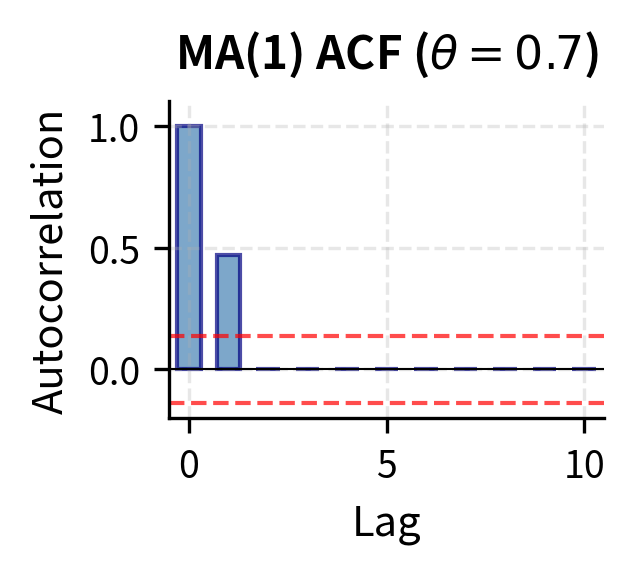
The ACF is therefore:
where:
- : autocorrelation at lag
- : moving average coefficient
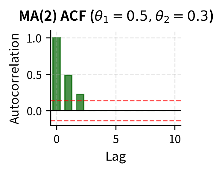
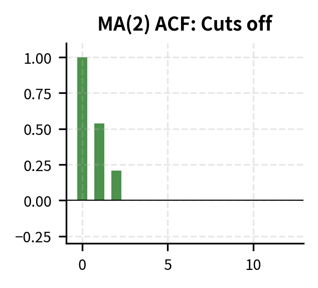
This cutoff property of the ACF is the diagnostic signature of MA models. An MA(q) process has for all , meaning the autocorrelation function drops abruptly to zero after lag . This sharp cutoff contrasts with the gradual decay of AR models and provides the basis for identifying MA order from sample ACF plots.
General MA(q) Models
The MA(q) model extends to include lagged shock terms:
where:
- : value of the series at time
- : constant mean
- : white noise shock at lag
- : moving average coefficient at lag
Using the lag operator:
where:
- : value of the series at time
- : moving average polynomial
- : constant mean
- : white noise series
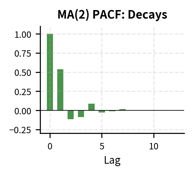
The moving average polynomial captures the distributed impact of shocks over time. The ACF cuts off after lag , while the PACF decays gradually. This is the opposite pattern from AR models. When we observe sample ACF with a sharp cutoff and PACF with gradual decay, this strongly suggests an MA process.
Invertibility
An MA model is invertible if it can be expressed as an AR() process, meaning we can write current shocks in terms of past observations. For MA(1), invertibility requires . The importance of invertibility goes beyond mathematical elegance. Non-invertible MA models create identification problems: an MA(1) with parameter and another with parameter produce identical autocorrelation structures, making the models observationally equivalent. By convention, we restrict attention to invertible representations to ensure unique parameter estimates.
ARMA Models: Combining AR and MA
Real financial time series often exhibit both autoregressive and moving average characteristics. Neither pure AR nor pure MA models may adequately capture the dependence structure. The ARMA(p,q) model combines both components:
where:
- : value of the series at time
- : constant term
- : autoregressive coefficients
- : moving average coefficients
- : white noise terms
In lag operator notation:
where:
- : autoregressive polynomial
- : constant term
- : moving average polynomial
Why Combine AR and MA?
The principle of parsimony motivates ARMA. Sometimes a pure AR model requires many lags to capture the autocorrelation structure, but a mixed ARMA model achieves the same fit with fewer parameters. This parsimony matters for both statistical and practical reasons. Models with fewer parameters are easier to interpret, more stable to estimate, and less prone to overfitting.
Consider an AR(1) process. Its ACF decays geometrically. An MA() could replicate this pattern, but that would require infinitely many parameters. Conversely, an MA(1) has an ACF that cuts off after lag 1, but an AR() could approximate it. ARMA provides flexibility to match complex autocorrelation patterns economically, using a small number of AR and MA terms to capture structures that would require many terms in either pure representation.
ARMA(1,1) Example
The ARMA(1,1) specification combines the first-order properties of both models, providing a rich but still tractable framework:
where:
- : value of the series at time
- : value of the series at time
- : constant term
- : autoregressive coefficient
- : moving average coefficient
- : white noise error term
- : white noise error term at time
Its ACF starts at:
where:
- : autocorrelation at lag 1
- : AR coefficient
- : MA coefficient
and then decays geometrically following the AR structure:
where:
- : autocorrelation at lag
- : autoregressive coefficient
- : autocorrelation at lag
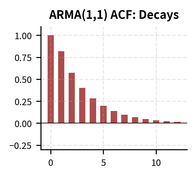
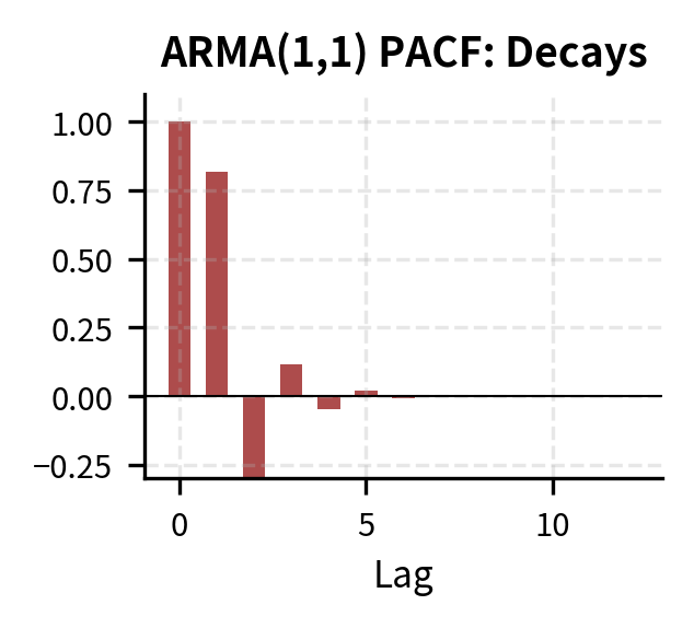
The MA component affects only the starting value of the autocorrelation sequence, while the AR component determines the rate of decay. The PACF also decays rather than cutting off, which is characteristic of processes with MA components. This makes ARMA models harder to identify than pure AR or MA processes, since neither the ACF nor PACF shows a clean cutoff pattern.
Stationarity and Invertibility
An ARMA(p,q) model is:
- Stationary if all roots of lie outside the unit circle
- Invertible if all roots of lie outside the unit circle
We typically work only with stationary and invertible representations. Stationarity ensures the process has stable statistical properties, while invertibility ensures unique parameter identification and allows us to recover the underlying shocks from observed data.
ARIMA Models: Handling Non-Stationarity
When the original series is non-stationary, such as asset prices or GDP, we can often achieve stationarity through differencing. Rather than modeling the original series directly, we model the changes. The ARIMA(p,d,q) model applies ARMA(p,q) to a -times differenced series, combining differencing to achieve stationarity with ARMA to model the resulting stationary dynamics.
The Differencing Operator
Define the difference operator , which computes the change from one period to the next:
where:
- : difference operator
- : value at time
- : value at time
For financial prices, first differencing yields returns. If the original price series has a unit root (is I(1)), then returns will be stationary. Second differencing applies the operator twice:
where:
- : second difference of the series
- : value at time
- : value at time
- : value at time
Second differencing is occasionally needed for economic series with both a unit root and a time-varying trend, though over-differencing can introduce artificial patterns and should be avoided.
ARIMA(p,d,q) Specification
An ARIMA(p,d,q) model states that follows an ARMA(p,q). The integrated component handles the transformation to stationarity, while the ARMA component models the resulting stationary dynamics. We can express this using the difference operator or the lag operator explicitly:
where:
- : value of the series at time
- : difference operator
- : AR polynomial
- : differencing operator of order
- : constant term
- : MA polynomial
- : white noise error term
Common specifications include:
- ARIMA(0,1,0): Random walk
- ARIMA(0,1,1): Random walk plus MA(1) on returns
- ARIMA(1,1,0): AR(1) on returns (first differences)
- ARIMA(1,1,1): ARMA(1,1) on returns
Drift in ARIMA Models
When , the constant induces a deterministic trend in the original series. For ARIMA(0,1,0) with constant:
where:
- : value of the series at time
- : value at time
- : constant term (drift)
- : white noise error term
This says that each period, the series increases by on average plus a random shock. Summing the increments from to reveals the cumulative effect of the drift and shocks:
where:
- : value at time
- : initial value
- : deterministic trend component
- : stochastic trend component
The term is a linear trend that grows steadily with time. The accumulated shocks form a stochastic trend that wanders randomly. This is the random walk with drift model, commonly used for log stock prices. It captures the empirical observation that stock prices tend to rise over time (positive drift) while exhibiting substantial random variation around this trend.
Model Identification
Identifying the appropriate specification is both art and science. The Box-Jenkins methodology provides a systematic approach.
Step 1: Assess Stationarity
First, examine the series visually and statistically:
- Visual inspection: Does the series trend or wander? Does variance appear stable?
- ACF analysis: For non-stationary series, the ACF decays very slowly
- Unit root tests: The Augmented Dickey-Fuller (ADF) test formally tests for stationarity
If the series is non-stationary, difference it and repeat. Most financial price series require (returns), while some economic series may need .
Step 2: Examine ACF and PACF
For the stationary (possibly differenced) series:
| Model | ACF Pattern | PACF Pattern |
|---|---|---|
| AR(p) | Decays gradually | Cuts off after lag |
| MA(q) | Cuts off after lag | Decays gradually |
| ARMA(p,q) | Decays gradually | Decays gradually |
The ACF and PACF of financial returns often suggest low-order models. Daily stock returns typically show little autocorrelation in levels but significant autocorrelation in squared returns (addressed in the next chapter on volatility modeling).
Step 3: Estimate Candidate Models
Fit several plausible specifications and compare using information criteria:
where:
- : Akaike Information Criterion
- : Bayesian Information Criterion
- : maximized likelihood
- : number of parameters
- : sample size
Lower values indicate better models. BIC penalizes complexity more heavily and tends to select simpler models.
Step 4: Diagnostic Checking
After estimation, verify that residuals behave like white noise:\n\n- Ljung-Box test: Tests whether residual autocorrelations are jointly zero
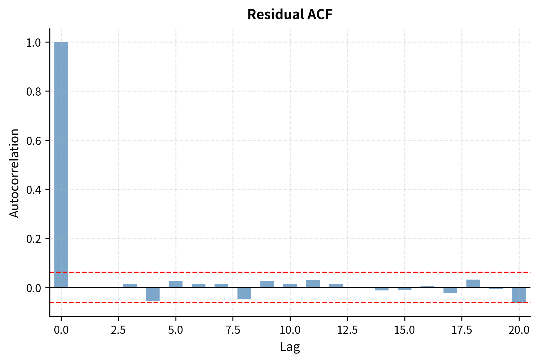
- Residual ACF: Should show no significant autocorrelations
- Normality tests: Check if residuals are approximately normal (though financial residuals often have fat tails)
If diagnostics fail, revisit the specification.
Forecasting with ARIMA Models
Time-series models are widely used for forecasting. Using observations up to time , we predict for horizons Forecast quality determines a model's practical value.
Point Forecasts
The optimal forecast (minimizing mean squared error) is the conditional expectation:
where:
- : forecast for time made at time
- : conditional expectation operator
- : future value at horizon
- : information set available at time
This conditional expectation uses all available information up to time to form the best prediction of the future value. For an AR(1) model , the one-step-ahead forecast is simply:
where:
- : one-step-ahead forecast
- : constant term
- : autoregressive coefficient
- : last observed value
For longer horizons, we iterate the forecasting equation, replacing unknown future values with their forecasts:
where:
- : two-step-ahead forecast
- : one-step-ahead forecast
- : constant term
- : autoregressive coefficient
- : last observed value
More generally, the forecast formula reveals how the current observation influences predictions at any horizon:
where:
- : forecast for given information at
- : unconditional mean
- : AR coefficient
- : forecast horizon
The forecast is a weighted average of the unconditional mean and the current deviation from that mean. The weight on the current deviation is , which shrinks toward zero as the horizon increases. As , forecasts converge to the unconditional mean: . This reflects the fundamental property that for stationary series, distant future values are increasingly disconnected from current conditions.
Forecast Intervals
The forecast error at horizon is the difference between the realized value and our prediction:
where:
- : forecast error at horizon
- : realized value at time
- : forecast made at time
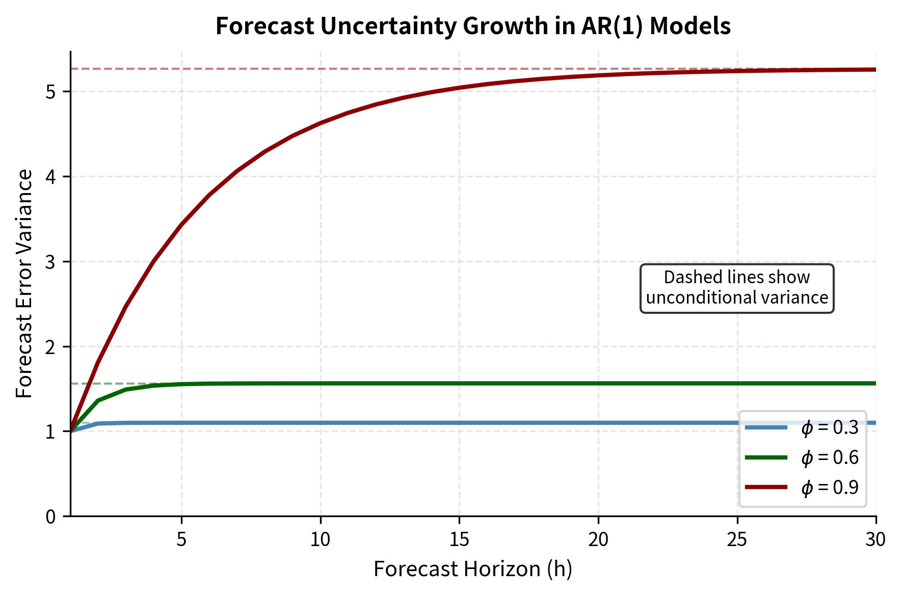
For AR(1), the forecast error variance grows with horizon as uncertainty accumulates:
where:
- : variance of the forecast error at horizon
- : innovation variance
- : AR coefficient
As , this converges to the unconditional variance . The uncertainty approaches the unconditional variance because at very long horizons, our conditional forecast converges to the unconditional mean, and the forecast error becomes essentially the deviation of the future observation from that mean.
A 95% forecast interval is:
where:
- : forecast for time given information at
- : z-score for 95% confidence
- : forecast error variance
This widening of forecast intervals reflects increasing uncertainty at longer horizons, a fundamental feature of time-series prediction. The honest acknowledgment of forecast uncertainty is crucial for risk management and decision-making under uncertainty.
Implementation: Analyzing S&P 500 Returns
Let's apply these concepts to real financial data, analyzing daily S&P 500 returns.
Simulating Financial Data
We'll work with a simulated dataset that mimics S&P 500 characteristics, then show how to identify and fit ARIMA models.
Visualizing Prices vs. Returns
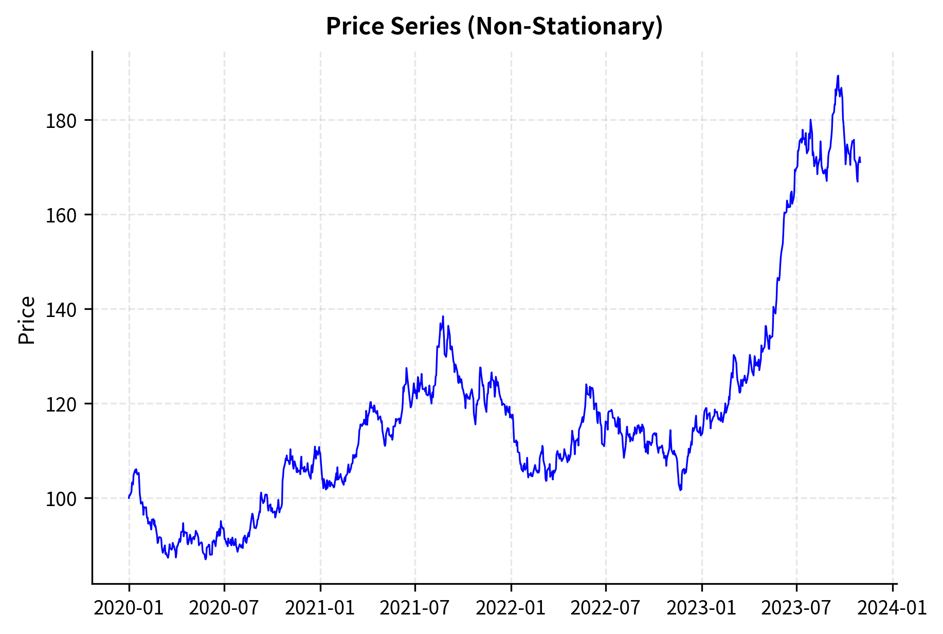
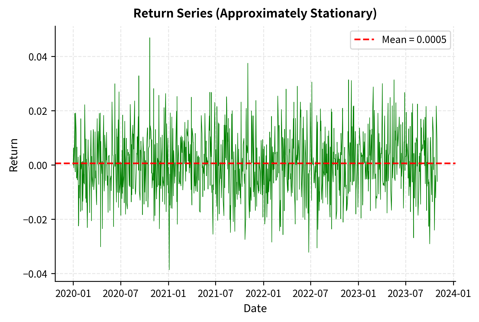
The price series shows a clear upward trend, violating the constant mean requirement for stationarity. Returns, however, fluctuate around a stable mean near zero, making them suitable for ARMA modeling.
Computing ACF and PACF
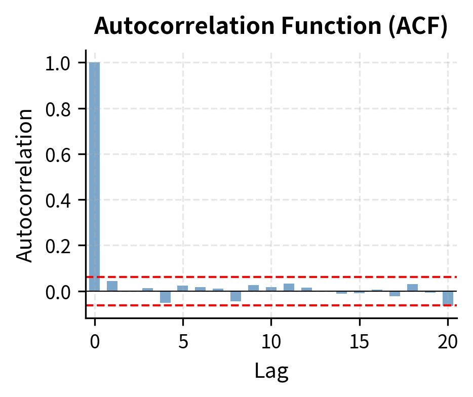
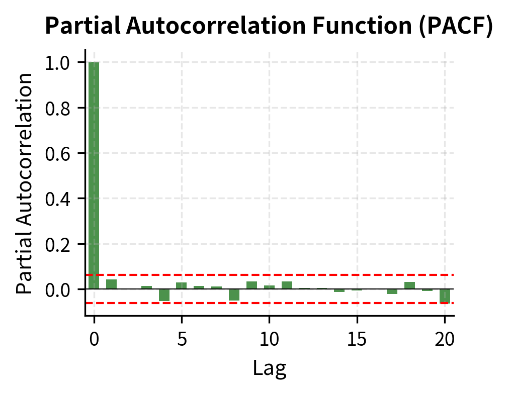
The ACF shows the lag-1 autocorrelation is significant, with subsequent lags decaying. The PACF shows a significant spike at lag 1 followed by values within the confidence bands. This pattern, with PACF cutting off after lag 1 and ACF decaying, strongly suggests an AR(1) model.
Estimating an AR(1) Model
We'll estimate the AR(1) parameters using ordinary least squares, which is consistent for stationary AR models.
The estimated AR(1) coefficient is close to our simulated value of 0.05. The model is stationary since .
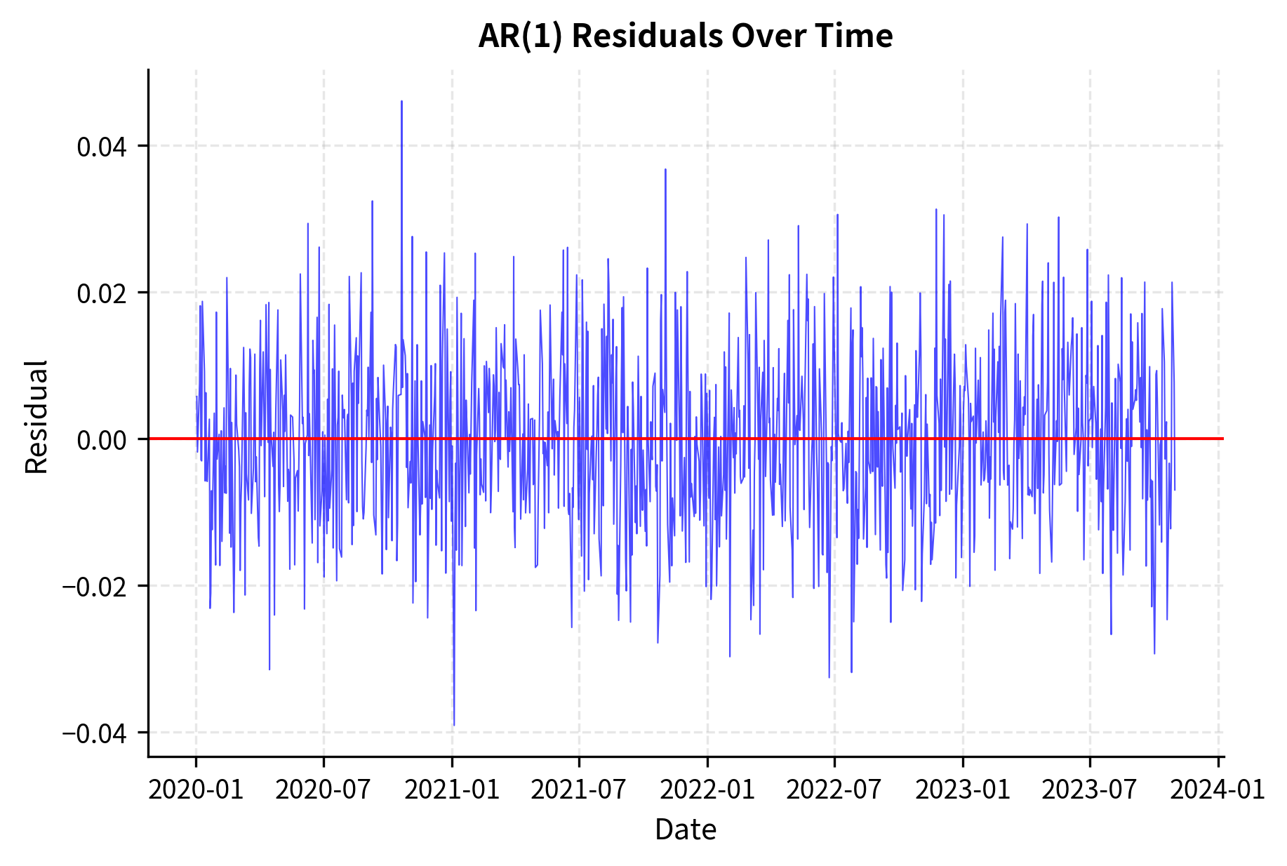
Diagnostic Checking
The Ljung-Box test checks whether residual autocorrelations are collectively significant. A high p-value suggests the residuals behave like white noise, indicating an adequate model.
Forecasting
With the estimated model, we can generate forecasts with confidence intervals.
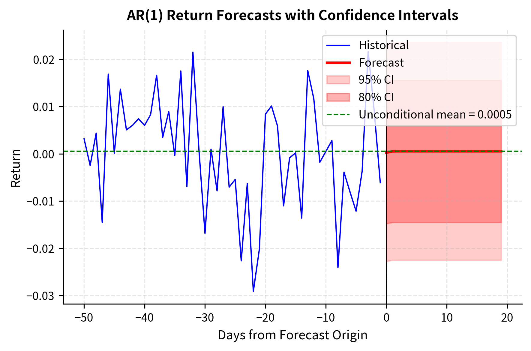
The forecasts converge quickly to the unconditional mean because the AR(1) coefficient is small. The confidence intervals widen initially but stabilize as they approach the unconditional variance.
Using statsmodels for ARIMA
In practice, we use established libraries for ARIMA estimation. The statsmodels package provides comprehensive time-series functionality.
The ADF test strongly rejects the null hypothesis of a unit root, confirming that returns are stationary and suitable for ARMA modeling without differencing.
Information criteria help select the best model balancing fit and parsimony. The BIC, with its heavier penalty for complexity, often selects simpler models appropriate for financial data.
The model summary confirms that the AR(1) coefficient is statistically significant and close to the true value of 0.05. The low p-values indicate strong evidence against zero coefficients.
ARIMA for Price Series
When working with prices directly, we need ARIMA with . This models returns (first differences) using ARMA.
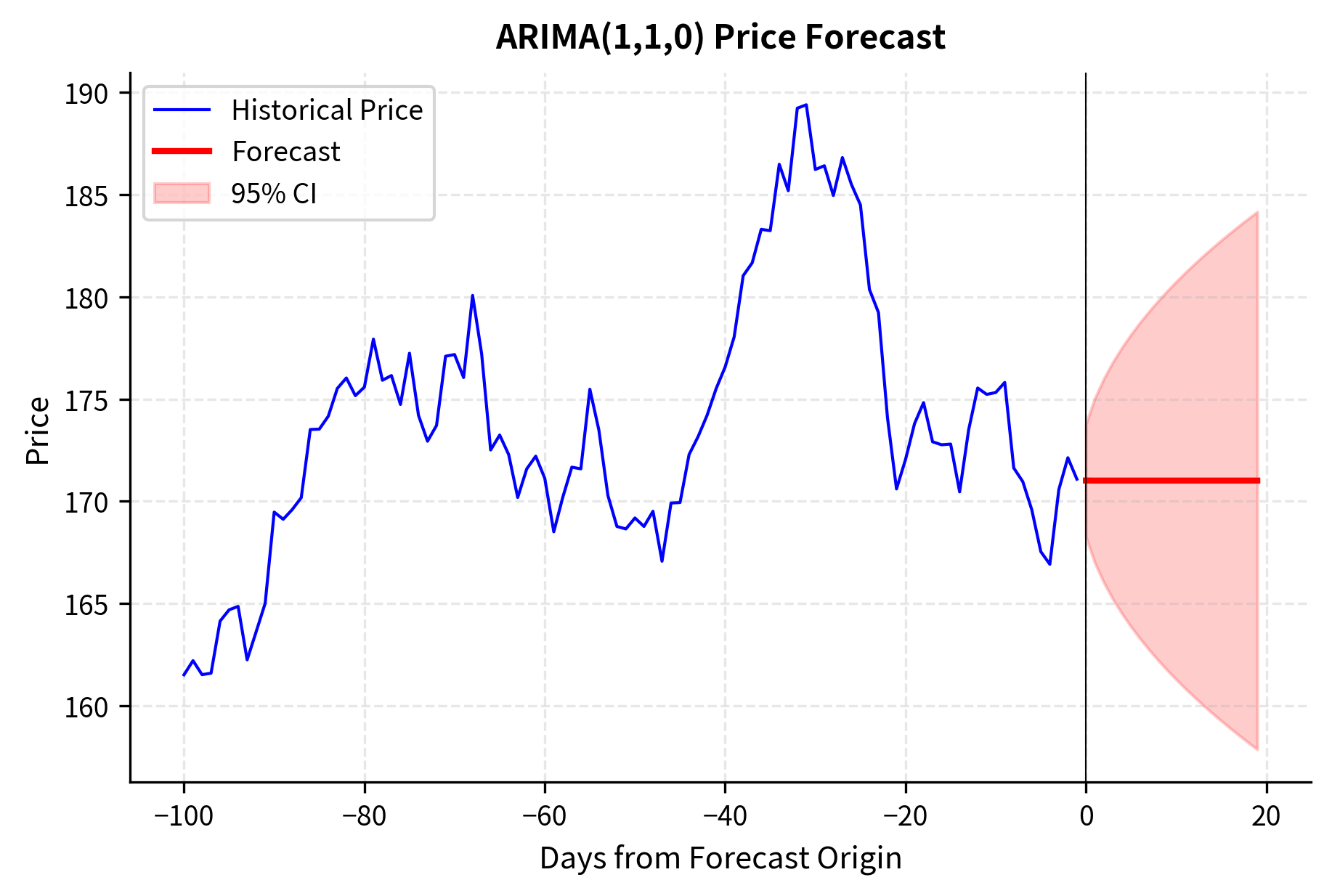
The confidence interval for price forecasts widens dramatically compared to return forecasts. This reflects the accumulation of return forecast errors: uncertainty compounds over time when predicting integrated series.
Financial Applications of ARIMA Models
ARIMA models find practical application across several areas of quantitative finance. This section examines three key applications: exploiting mean-reverting behavior in spreads, quantifying risk through conditional forecasts, and projecting macroeconomic variables.
Mean Reversion Trading
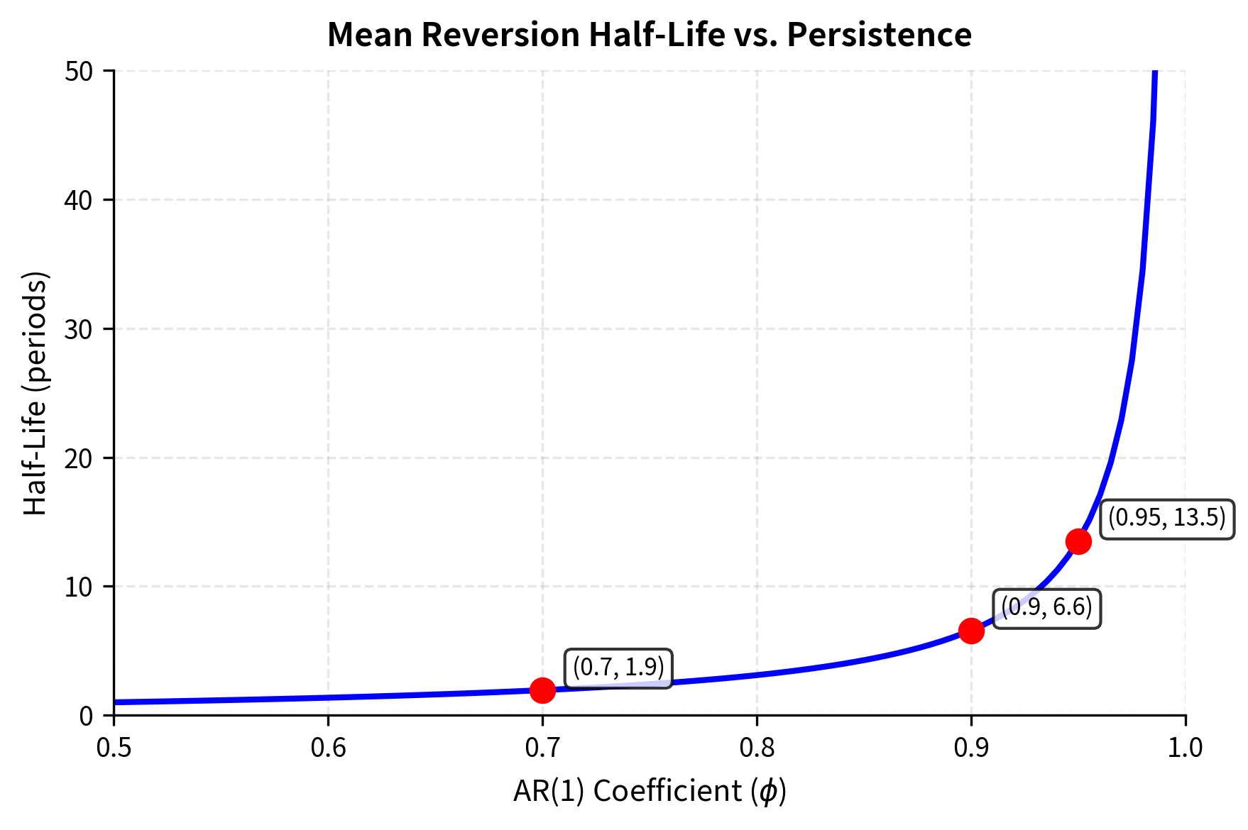
Interest rate spreads and basis trades often exhibit mean-reverting behavior well-captured by AR models. If a spread follows AR(1) with :
where:
- : spread at time
- : long-run mean spread
- : autoregressive coefficient (determines speed of reversion; must be )
- : random shock
When the spread deviates from , the expected deviation decays geometrically. The half-life measures the time required for this deviation to shrink by 50% (). Since the expected deviation at is , we solve:
where:
- : half-life of the mean reversion process
- : autoregressive coefficient
For , the half-life is approximately 13.5 periods.
Risk Management
ARIMA forecasts provide inputs for Value-at-Risk calculations. The conditional distribution of future returns:
where:
- : distribution of returns at conditional on time
- : conditional expected return
- : conditional forecast variance
allows computation of forward-looking VaR that accounts for current conditions rather than using unconditional distributions.
Economic Forecasting
Central bank policy analysis uses ARIMA models for inflation, GDP growth, and employment forecasts. These series often require or and seasonal components (SARIMA) that extend the basic ARIMA framework.
Limitations and Practical Considerations
Time-series models help analyze serial dependence, but they have limitations with financial data.
Linear structure assumption: ARMA models capture only linear dependencies. As we observed in the chapter on stylized facts, financial returns exhibit significant nonlinear features. While squared returns may be highly autocorrelated (indicating predictable volatility patterns), raw returns often show minimal linear autocorrelation. This means ARMA models may suggest returns are nearly unpredictable when substantial predictability exists in higher moments. The next chapter on GARCH models addresses this limitation by modeling the conditional variance process.
Stationarity requirements: The assumption that the data-generating process remains stable over time is often violated in financial markets. Structural breaks occur due to regulatory changes, market crises, and regime shifts. An ARIMA model estimated on pre-2008 data would perform poorly during the financial crisis. Adaptive estimation windows and regime-switching models partially address this, but no mechanical solution exists for genuine structural change.
Gaussian innovations: The standard ARIMA framework assumes normally distributed innovations, yet financial returns consistently exhibit fat tails. This matters most for risk applications: forecast intervals based on normal distributions systematically underestimate tail risk. Using Student-t or other fat-tailed distributions for the innovation process improves this, though at the cost of added complexity.
Limited forecasting horizon: For typical equity returns with autocorrelation coefficients near zero, ARIMA models provide little forecasting value. The optimal forecast quickly converges to the unconditional mean. Where ARIMA models excel is in series with genuine persistent dynamics: interest rate spreads, volatility measures (the square of returns), and macroeconomic indicators.
Model selection uncertainty: The Box-Jenkins methodology requires judgment calls about differencing order, lag selection, and handling of outliers. Different practitioners may arrive at different specifications from the same data. Information criteria help but don't eliminate subjectivity. In high-frequency trading applications, this model uncertainty itself becomes a risk factor.
Despite these limitations, ARIMA models established the foundation for modern financial time-series analysis. The concepts of stationarity, autocorrelation structure, and systematic model identification remain central even as we extend to more sophisticated approaches.
Summary
This chapter developed the theory and practice of time-series modeling for financial data. We established stationarity as the foundational property enabling meaningful statistical analysis and showed that while asset prices are non-stationary, returns typically achieve approximate stationarity.
Autoregressive models express current values as linear functions of past values, with the AR coefficient controlling the persistence of shocks. The stationarity condition ensures the series remains bounded, while the PACF's cutoff property identifies AR order. Moving average models instead express observations as functions of past innovations, with the ACF cutting off after lag . ARMA combines both structures for parsimonious modeling of complex autocorrelation patterns.
For non-stationary series, ARIMA extends the framework through differencing. The integrated component handles trends and unit roots common in economic and price data. The Box-Jenkins methodology provides a systematic approach: assess stationarity, examine ACF/PACF patterns, estimate candidate models, compare using information criteria, and verify through residual diagnostics.
Forecasting from ARIMA models produces point predictions and uncertainty intervals that widen with horizon. This quantification of forecast uncertainty is essential for risk management applications. The tools developed here, particularly ACF analysis and model diagnostics, will prove valuable throughout the remainder of this book as we explore volatility modeling, regression methods, and machine learning approaches to financial prediction.
Quiz
Ready to test your understanding? Take this quick quiz to reinforce what you've learned about time-series models for financial data.

Comments