

Master credit risk modeling from Merton's structural framework to reduced-form hazard rates and Gaussian copula portfolio models with Python implementations.
Choose your expertise level to adjust how many terms are explained. Beginners see more tooltips, experts see fewer to maintain reading flow. Hover over underlined terms for instant definitions.
Credit Risk Modeling Approaches
Credit risk modeling transforms qualitative assessments of borrower creditworthiness into quantitative estimates of default probability, loss given default, and portfolio risk. Building on the credit risk fundamentals from the previous chapter, we explore the mathematical frameworks that underpin modern credit risk management.
Two philosophically different approaches dominate the field: structural models and reduced-form models. Structural models, pioneered by Robert Merton in 1974, view default as an economic event driven by the firm's asset value falling below its debt obligations. These models use option pricing theory from Part III to treat equity as a call option on the firm's assets. Reduced-form models take a different path, modeling default as a random event governed by a hazard rate process without explicitly modeling the firm's balance sheet, connecting directly to the credit default swap pricing we covered in Part II.
Beyond individual obligor models, credit risk managers must assess portfolio-level risk. A portfolio of 1,000 loans does not have 1,000 times the risk of a single loan because defaults are correlated. Economic downturns cause multiple borrowers to default simultaneously. Portfolio credit risk models like CreditMetrics and the Gaussian copula framework capture these dependencies, enabling calculation of credit Value-at-Risk (VaR) for loan portfolios.
This chapter develops each approach from first principles with working implementations, preparing you to build credit risk systems that combine theoretical rigor with practical applicability.
Structural Models: The Merton Framework
Structural models derive default probability from the fundamental economics of a firm's capital structure. The key insight is straightforward: shareholders hold a residual claim on the firm's assets after debt is paid. If assets exceed debt at maturity, shareholders receive the difference. If assets fall short, they walk away with nothing while creditors absorb the loss. This simple observation, when combined with the machinery of option pricing theory, yields a powerful framework for quantifying credit risk.
Equity as a Call Option on Assets
To understand the Merton framework, recognize the option-like nature of equity in a leveraged firm. Consider a firm with total asset value financed by equity and zero-coupon debt with face value maturing at time . At maturity, the firm's assets must be distributed between debt holders and equity holders according to the priority of claims established by corporate law. Debt holders have senior claims and must be paid first. Only after debt is fully satisfied do equity holders receive any value.
This priority structure means that at maturity, the payoff to equityholders is:
where:
- : equity value at maturity
- : total firm asset value at maturity
- : face value of debt (the strike price of the option)
- : time to maturity in years
- : equityholders receive the residual after paying debt, or nothing if assets are insufficient
This payoff structure is precisely that of a European call option on the firm's assets with strike price . The analogy reveals deep insights about how equity and debt behave. Equity holders enjoy limited downside. They can walk away with nothing if the firm fails without being forced to inject additional capital. At the same time, equity holders have unlimited upside potential if assets appreciate significantly above the debt level. This asymmetry—the ability to participate in gains while limiting losses—is the defining characteristic of an option.
Debtholders' position is the complement of equity. Debtholders receive
where:
- : debt value at maturity
- : total firm asset value at maturity
- : face value of debt
- : debtholders receive the lesser of asset value or promised payment
- : payoff of a put option on assets struck at (represents credit risk)
- : decomposition showing debt equals risk-free bond minus a put option
The second form of this equation provides a crucial decomposition. The debt payoff equals the face value minus a put option on assets struck at D. This decomposition reveals that bondholders are effectively short a put option: the put option represents the credit risk embedded in corporate debt. When a firm defaults (assets fall below debt), bondholders suffer losses exactly equal to the intrinsic value of this embedded put. This insight transforms credit risk analysis into option pricing, allowing us to apply the tools developed for derivatives valuation.
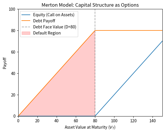
The shaded region in the figure shows where default occurs. When the terminal asset value falls below the debt face value, equity holders receive nothing, as their call option finishes out of the money. Meanwhile, debtholders recover only instead of the promised and absorb losses proportional to the shortfall. The visual representation makes clear why leverage matters: as debt increases relative to assets, the default region expands, and the probability of equity finishing worthless increases correspondingly.
The Merton Model Derivation
Now we develop the mathematical framework for valuing equity and debt while extracting default probabilities. The key modeling assumption is that asset value follows geometric Brownian motion under the physical measure:
where:
- : firm asset value at time
- : expected asset return (drift rate under the physical measure)
- : asset volatility, the standard deviation of asset returns
- : standard Brownian motion
- : infinitesimal Brownian increment
- : infinitesimal time increment
- : infinitesimal change in asset value over time
This stochastic differential equation describes asset dynamics with two components. The deterministic drift term μ V_t dt captures the expected appreciation of assets over time, reflecting the firm's earning power and investment returns. The stochastic term introduces randomness that scales with the current asset level, ensuring percentage changes in asset value have constant volatility regardless of the firm's size.
As we derived in Part III when developing Black-Scholes, this stochastic differential equation implies that asset returns are normally distributed, which means the terminal asset value has a lognormal distribution. Applying Itô's lemma to and integrating over the interval from 0 to yields:
where:
- : asset value at maturity time
- : current asset value
- and : natural logarithms of asset values
- : expected asset return (physical drift)
- : asset volatility
- : time to maturity in years
- : standard normal random variable,
- : drift adjustment accounting for Itô's lemma, the volatility drag that reduces geometric growth
- : total volatility (standard deviation) accumulated over period
- The formula shows that log asset returns are normally distributed with mean and variance
The drift adjustment term is important to understand. This correction arises from Itô's lemma and reflects the difference between arithmetic and geometric average returns. When returns are volatile, the geometric mean (which determines wealth accumulation) falls below the arithmetic mean by approximately half the variance, a phenomenon sometimes called volatility drag. This explains why highly volatile assets can have high expected returns yet still disappoint long-term investors.
The Merton model produces two default probabilities depending on the measure used. The physical default probability uses the actual asset drift and represents real-world default likelihood. The risk-neutral default probability uses the risk-free rate for pricing credit derivatives. The two differ by the market price of risk.
Now we can derive the default probability by working through the mathematical condition for default. Default occurs when , meaning assets at maturity are insufficient to cover debt obligations. We derive the default condition by starting from this inequality and substituting the lognormal distribution:
The derivation proceeds by first taking the logarithm of both sides, which is valid since both and are positive. Next, we substitute the expression for from our lognormal distribution result. Rearranging to isolate the random component on one side yields a threshold that must fall below for default to occur. Since is standard normal, the probability that default occurs is the probability that falls below this threshold. Defining the distance to default as:
The physical default probability is:
where:
- : distance to default measured in standard deviations, indicates how many standard deviations the asset value is above the default threshold
- : current asset value
- : debt face value (default barrier)
- : log moneyness, measuring the relative position of assets versus debt
- : risk-adjusted drift
- : time to maturity
- : total volatility over the horizon
- : cumulative distribution function of the standard normal distribution
- The sign flip from to accounts for taking the probability of the complementary event
The quantity d_2 is called the distance to default when measured in standard deviations. This terminology captures its intuitive interpretation: the parameter tells us how many standard deviations the expected log asset value is above the log default threshold. A higher d_2 means the firm is further from default: a larger adverse shock is required to trigger insolvency. A firm with would need assets to fall by more than three standard deviations to default, an event with very low probability under the normal distribution.
Valuing Equity and Debt
Having established the default probability framework, we now turn to valuation. Using the Black-Scholes framework from Part III Chapter 6, we can value equity as a European call option on the firm's assets. Since equity holders receive at maturity, and the underlying asset follows geometric Brownian motion, the current equity value equals the call option value:
where:
- : current equity value
- : current asset value
- : debt face value (strike price)
- : risk-free rate
- : time to maturity
- : cumulative standard normal distribution
- and : risk-neutral distance to default parameters (defined below)
- : present value of the asset value in scenarios where the option is exercised, weighted by delta
- : present value of the strike price payment, weighted by risk-neutral probability of exercise
- This is the standard Black-Scholes call option formula applied to equity as a call on firm assets
This formula has a clear economic interpretation: the first term represents the expected asset value received by equity holders in favorable scenarios, discounted and weighted by the hedge ratio. The second term represents the present value of the debt payment, weighted by the probability that equity finishes in the money. The difference captures the value of equity's limited liability and upside potential.
The parameters and are given by:
where:
- : current asset value
- : debt face value
- : risk-free rate (replaces in the risk-neutral measure)
- : asset volatility
- : time to maturity
- : measures moneyness adjusted for volatility and time
- : risk-neutral distance to default
- Superscript indicates risk-neutral (pricing) measure
- represents the risk-neutral probability that equity finishes in-the-money
The superscript indicates risk-neutral parameters, distinguishing them from the physical measure quantities: the key difference is that risk-neutral valuation replaces the physical drift with the risk-free rate , reflecting the fundamental theorem of asset pricing. Debt value can be decomposed as risk-free debt minus the embedded put option:
where:
- : current value of risky debt
- : debt face value
- : risk-free rate
- : time to maturity
- : current asset value
- : value of the put option on assets (credit risk component)
- : cumulative standard normal distribution
- : risk-neutral distance to default parameters
- : present value of the debt face value (risk-free component)
- : present value of debt payment in non-default scenarios
- : present value of asset recovery in default scenarios
- and : probabilities associated with default outcomes
This decomposition reveals the fundamental nature of credit risk. Corporate debt can be valued as risk-free debt minus a put option, where the put option represents the creditors' exposure to default. When assets fall below the debt face value, creditors receive only the asset value rather than the full promised payment. The difference between risk-free and risky debt value represents the credit spread that compensates lenders for bearing default risk. This spread increases with leverage, volatility, and time to maturity, exactly as the option framework predicts.
Implementation: The Merton Model
Let's implement the complete Merton model with both physical and risk-neutral default probabilities:
The distance to default of 2.44 standard deviations indicates the firm has moderate default risk. A higher distance indicates lower credit risk, as larger adverse shocks are required to trigger default. The risk-neutral default probability exceeds the physical probability because the risk-neutral drift (the risk-free rate) is lower than the physical drift (the expected asset return), making downward paths more likely under the pricing measure. This difference reflects the market price of risk. The credit spread compensates lenders for bearing this default risk.
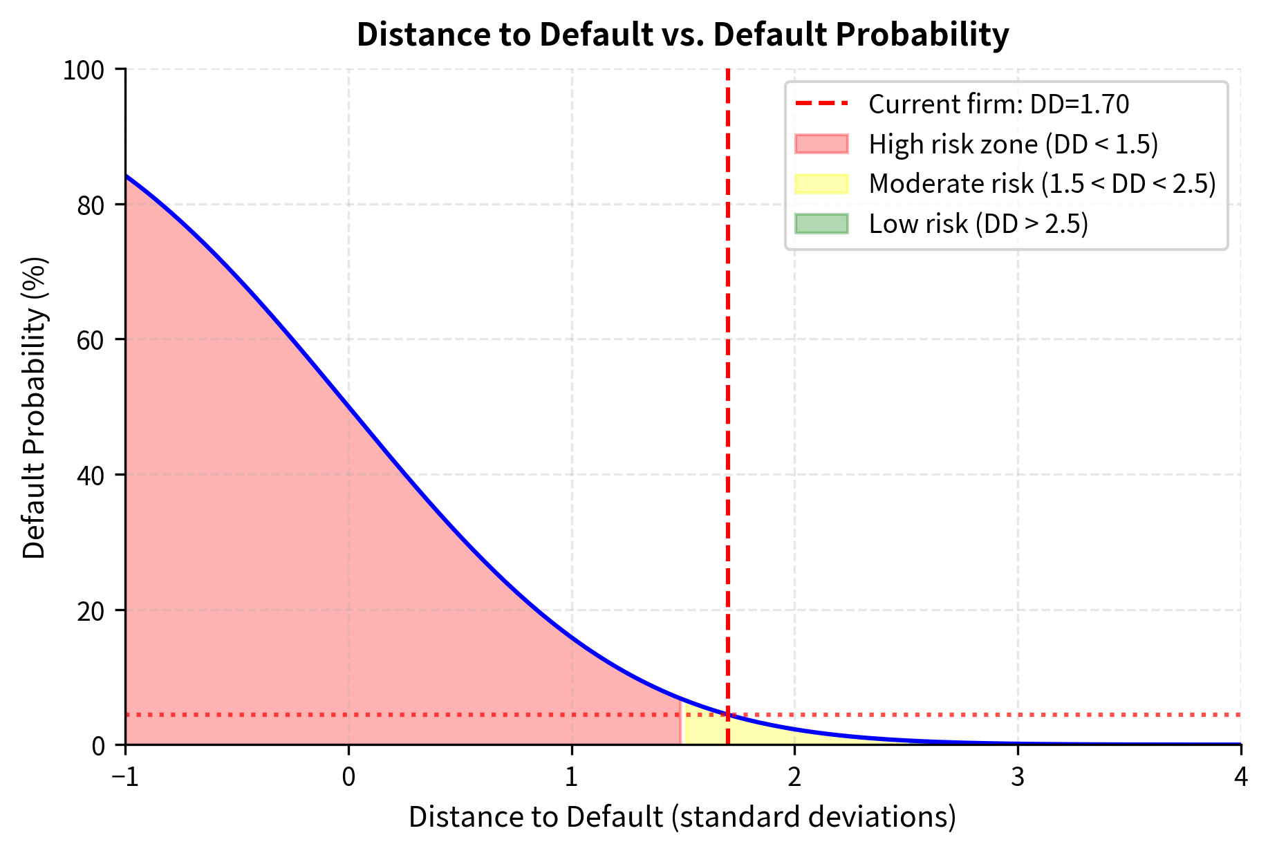
The figure illustrates how distance to default maps to default probability through the cumulative normal distribution. Firms with distance to default below 1.5 standard deviations face elevated default risk exceeding 7%, placing them in the high-risk zone. The moderate risk zone spans 1.5 to 2.5 standard deviations, with default probabilities between 0.6% and 7%. Firms with distance to default above 2.5 standard deviations are considered low risk, with default probability below 0.6%. Our example firm with distance to default of 2.44 sits at the boundary between moderate and low risk zones.
Key Parameters
These key parameters drive model behavior and credit risk dynamics.
- V0: Current firm asset value. This represents the total value of the firm's assets, including both tangible and intangible assets. Higher asset values relative to debt reduce default probability by increasing the buffer between current value and the default barrier.
- D: Face value of debt (the default barrier). This parameter determines the threshold that assets must exceed to avoid default. Higher debt increases leverage and default risk by raising the barrier that must be cleared.
- T: Time to maturity in years. Longer horizons increase uncertainty about future asset values and option value. The relationship with default probability is nuanced. Longer time allows both more opportunity for assets to appreciate and more opportunity for adverse shocks.
- sigma_V: Asset volatility. Higher volatility increases both equity value (through increased option value) and default probability (through increased probability of large adverse movements). This dual effect explains why equity holders may prefer higher volatility while debt holders prefer lower volatility.
- r: Risk-free rate. Used in the risk-neutral pricing measure for valuation purposes.
- mu: Expected asset return under the physical measure. Used for physical default probability calculations to assess real-world default risk.
Sensitivity Analysis
Credit risk depends critically on leverage and asset volatility. Let's examine how default probability varies with these parameters to build intuition for the model's behavior:
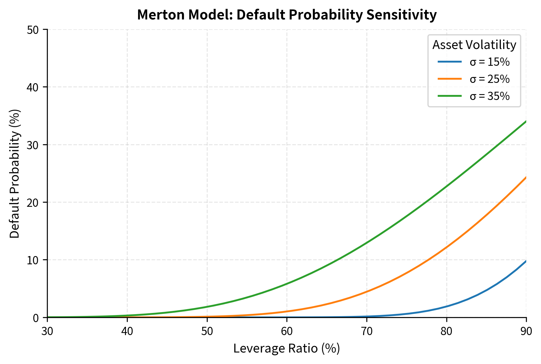
The nonlinear relationship between leverage and default probability reflects the option-like nature of credit risk. At low leverage (30-40%), even large changes in the leverage ratio have minimal impact on default probability, remaining below 5% even at 25% volatility. This corresponds to deeply in-the-money equity options where the probability of finishing out of the money is negligible. As leverage increases beyond 60%, credit risk rises exponentially. This acceleration occurs because the equity option moves from deep in-the-money toward at-the-money, where option values are most sensitive to changes in moneyness. At 80% leverage with 35% volatility, default probability reaches nearly 40%, consistent with the behavior of deep out-of-the-money options becoming at-the-money. The interaction between leverage and volatility is also apparent: at low leverage, volatility has modest effects, but at high leverage, the difference between 15% and 35% volatility represents the difference between manageable and severe default risk.
Estimating Unobservable Asset Value and Volatility
The Merton model's key practical challenge is that asset value and asset volatility are not directly observable. While equity prices trade on public exchanges, a firm's total asset value includes intangible assets, growth options, and synergies that cannot be directly measured. We observe equity value (market capitalization) and equity volatility from option prices or historical returns. We invert the model to recover asset parameters from these observables.
Applying Itô's lemma (as we did when deriving the Black-Scholes PDE in Part III), we can derive how equity volatility relates to asset volatility through the chain rule of stochastic calculus:
where:
- : equity volatility (observable from market prices)
- : asset volatility (unobservable, must be estimated)
- : equity value
- : asset value
- : delta of the equity call option, equal to
- : leverage ratio in the option context
- : the option delta, measuring sensitivity of equity value to asset value changes
- The product represents the leverage multiplier: equity volatility exceeds asset volatility because equity is a levered claim
This relationship captures the leverage effect in credit markets. Since equity represents a call option on assets, small percentage changes in asset value are magnified into larger percentage changes in equity value. The leverage multiplier exceeds one for leveraged firms, explaining why equity volatility typically exceeds asset volatility. A highly leveraged firm near default will have extremely high equity volatility even if asset volatility is moderate, because small asset fluctuations translate into large percentage changes in the thin equity cushion.
This gives us two equations to work with:
- Equity pricing:
- Volatility relationship:
Both equations involve the same unknowns ( and ), and both can be expressed using market observables (, , , , ). We solve this system numerically:
The estimation successfully backs out the unobservable asset parameters from market data. The estimated asset value of approximately 35 million by the present value of debt, confirming the accounting identity that assets equal equity plus debt. The estimated asset volatility of around 25% is roughly half the equity volatility of 50%, reflecting the leveraging effect where debt acts as a fixed obligation that amplifies equity movements. Think of a seesaw: if total assets move by 1%, equity (the smaller end) must move by proportionally more to maintain balance. The resulting 69% leverage ratio and distance to default around 1.7 standard deviations indicate moderate credit risk, translating to a physical default probability near 4% and credit spread around 150 basis points.
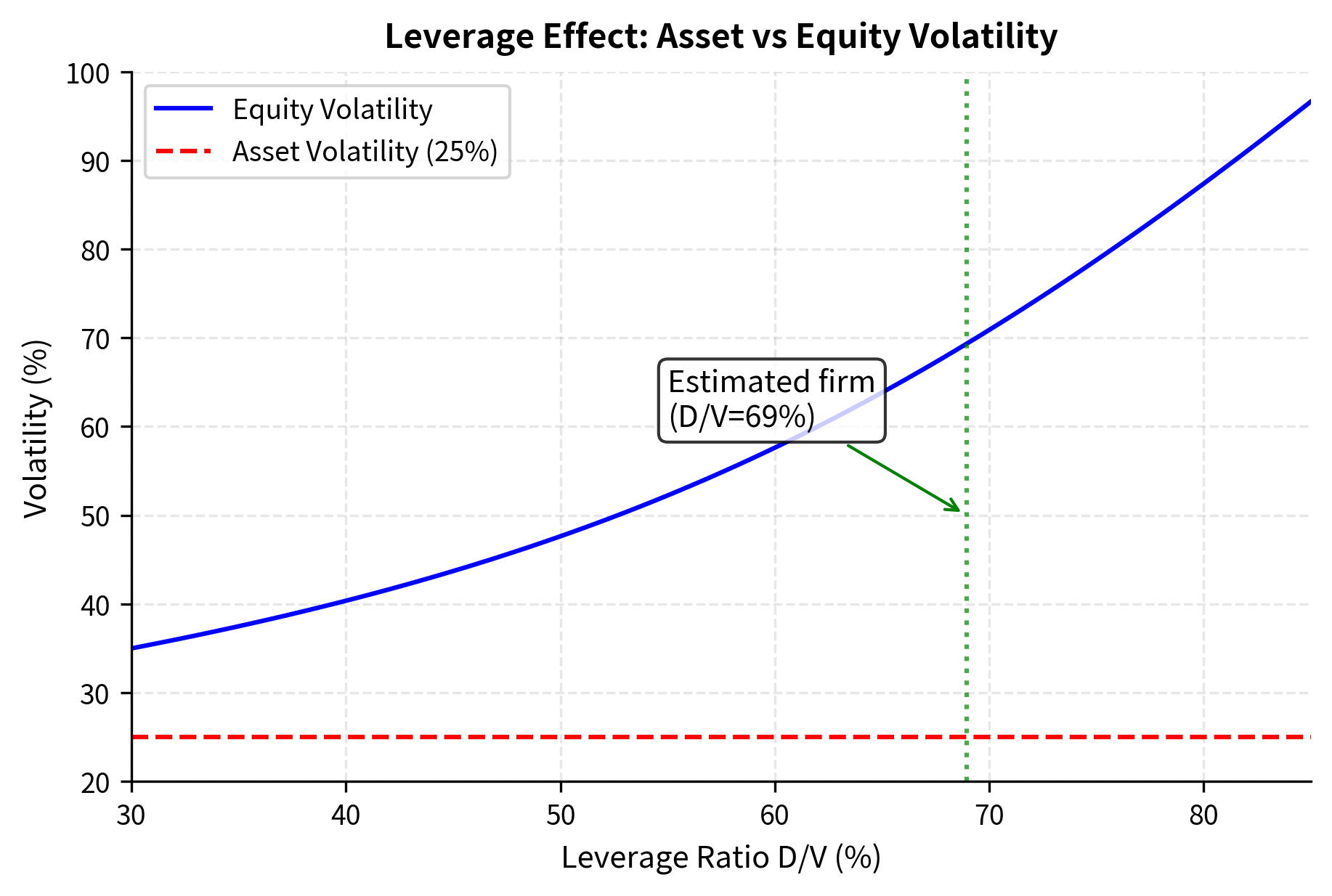
The leverage effect visualization demonstrates why equity volatility systematically exceeds asset volatility for leveraged firms. At 30% leverage, equity volatility is only slightly above asset volatility because the equity cushion is substantial. As leverage increases, the equity cushion shrinks, and any percentage change in asset value translates into a proportionally larger percentage change in equity value. At 80% leverage, equity volatility reaches nearly three times asset volatility. This relationship has important implications for credit risk assessment: when estimating asset volatility from equity volatility, failing to account for the leverage effect would substantially overestimate asset risk.
Reduced-Form Models: Intensity-Based Approach
Reduced-form models take a fundamentally different approach from structural models. Rather than deriving default from balance sheet dynamics and capital structure, they model default as a random event governed by a hazard rate (or default intensity). Default occurs exogenously, without explicit modeling of economic mechanisms. Instead of asking why the firm defaults, reduced-form models focus on when: estimating the instantaneous default probability at any moment given that the firm has survived to that time.
This approach offers several practical advantages. First, it's easier to calibrate to market prices since the hazard rate connects directly to observable credit spreads. Second, the framework handles multiple credit events naturally (including rating downgrades and restructurings), not just binary default. Third, it doesn't require unobservable asset values, making implementation more straightforward.
The Hazard Rate Framework
The mathematical foundation of reduced-form models rests on the concept of a hazard rate, which originates from survival analysis in statistics and actuarial science. The default time is the first time a default-triggering event occurs. The survival probability to time is the likelihood that the obligor remains solvent through time :
where:
- : probability of surviving (not defaulting) until time
- : random default time
- : probability that default occurs after time
The survival probability function captures the declining likelihood of remaining solvent as time progresses. It starts at (the firm is solvent today) and decreases toward zero as the time horizon extends (eventually all firms default or cease to exist). The rate at which this probability declines at any moment is governed by the hazard rate.
The hazard rate (or default intensity) represents the instantaneous probability of default given survival to time :
where:
- : hazard rate (default intensity) at time
- : random default time
- : current time
- : small time increment
- : conditional probability of defaulting in the interval , given survival to time
- The limit as gives the instantaneous default rate
The hazard rate is the conditional rate of default for a firm that has survived until time .
The hazard rate has an intuitive interpretation as the instantaneous default probability per unit time: if the hazard rate is 5% per year, it means that at any moment, a firm that has survived faces approximately a 5% chance of defaulting over the next year. The conditioning on survival is crucial: we only ask about default probability for firms that haven't already defaulted.
The survival probability relates to the hazard rate through the exponential of the cumulative hazard. To see why, note that the survival probability must satisfy because the rate of decrease in survival probability equals the hazard rate times the probability of having survived so far. This differential equation simply states that the rate at which firms leave the surviving population equals the hazard rate times the population size. Solving this differential equation with initial condition gives:
where:
- : survival probability to time
- : hazard rate (default intensity) at time
- : integration variable representing time from 0 to
- : cumulative hazard, the total default risk accumulated from time 0 to
- : exponential function
- The exponential function converts cumulative hazard to survival probability through the relationship
- This relationship follows from solving the differential equation with initial condition
The integral represents the cumulative hazard, capturing the total default risk accumulated from time 0 to time . The exponential transformation converts this accumulated risk into a survival probability. Higher cumulative hazard means lower survival probability, with the exponential ensuring the probability remains between 0 and 1.
For a constant hazard rate , this simplifies to:
where the integral becomes simply , giving exponential decay in survival probability. This exponential decay is the hallmark of the constant hazard model: the survival probability decreases at a rate proportional to itself.
The cumulative default probability is:
where:
- : probability of defaulting by time
- : random default time
- : survival probability with constant hazard
- : complement gives cumulative default probability
Connection to Poisson Processes
The constant hazard rate model implies default arrives as a Poisson process with intensity . This connection provides deep insight into reduced-form model mechanics. The Poisson process describes events that occur randomly over time with a constant average rate, and the exponential distribution characterizes the waiting time until the first such event.
The key property of the Poisson process is the memoryless property. Given that a firm has survived to time , the probability distribution of remaining time to default is the same as if we started fresh at time zero. This may seem counterintuitive (shouldn't older firms be closer to default?), but it captures the idea that conditional on survival, the firm faces the same ongoing default intensity. The waiting time until default follows an exponential distribution with mean , so a firm with a 2% annual hazard rate has an expected time to default of 50 years, though actual default could occur much sooner or later due to the high variance of exponential distributions.
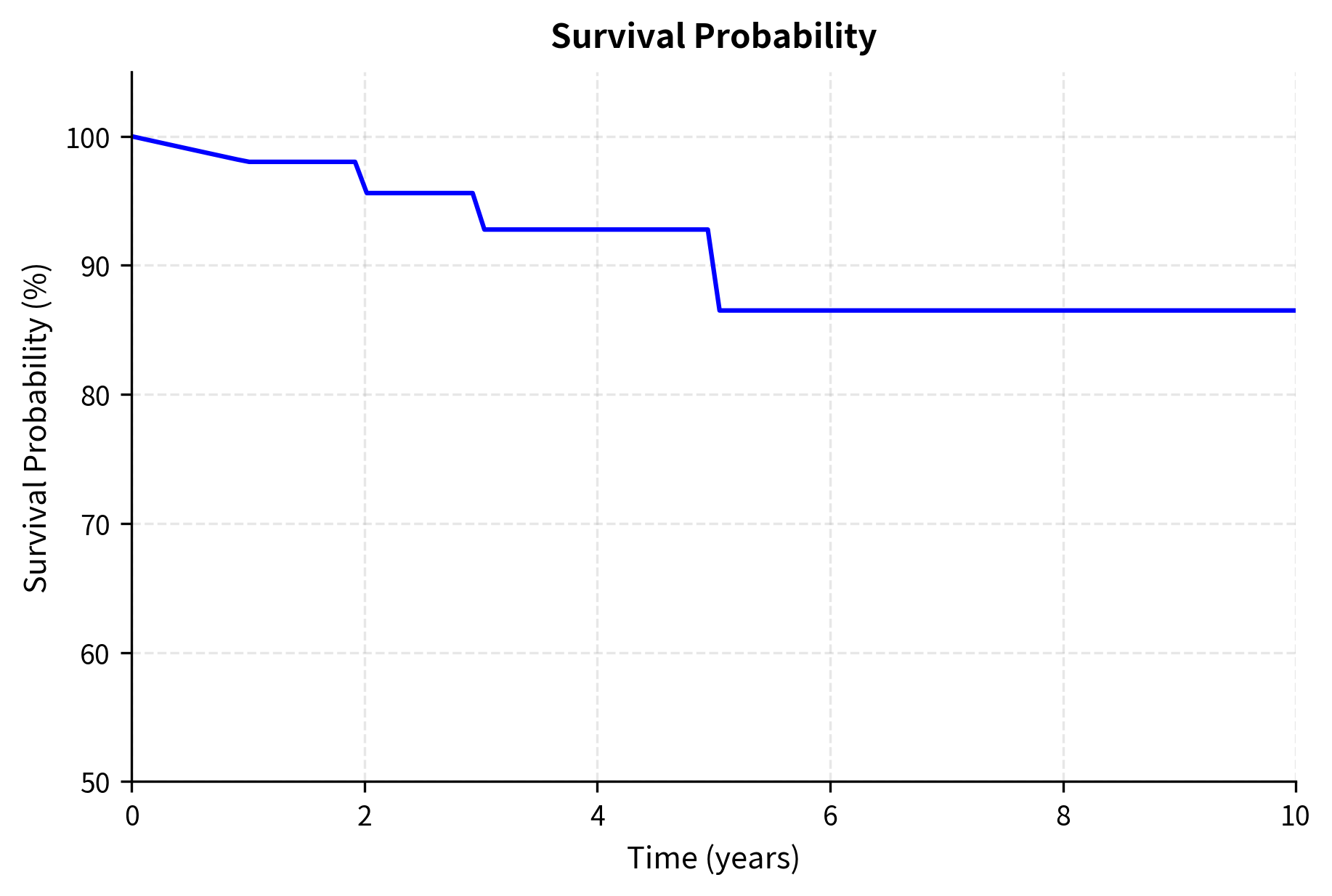
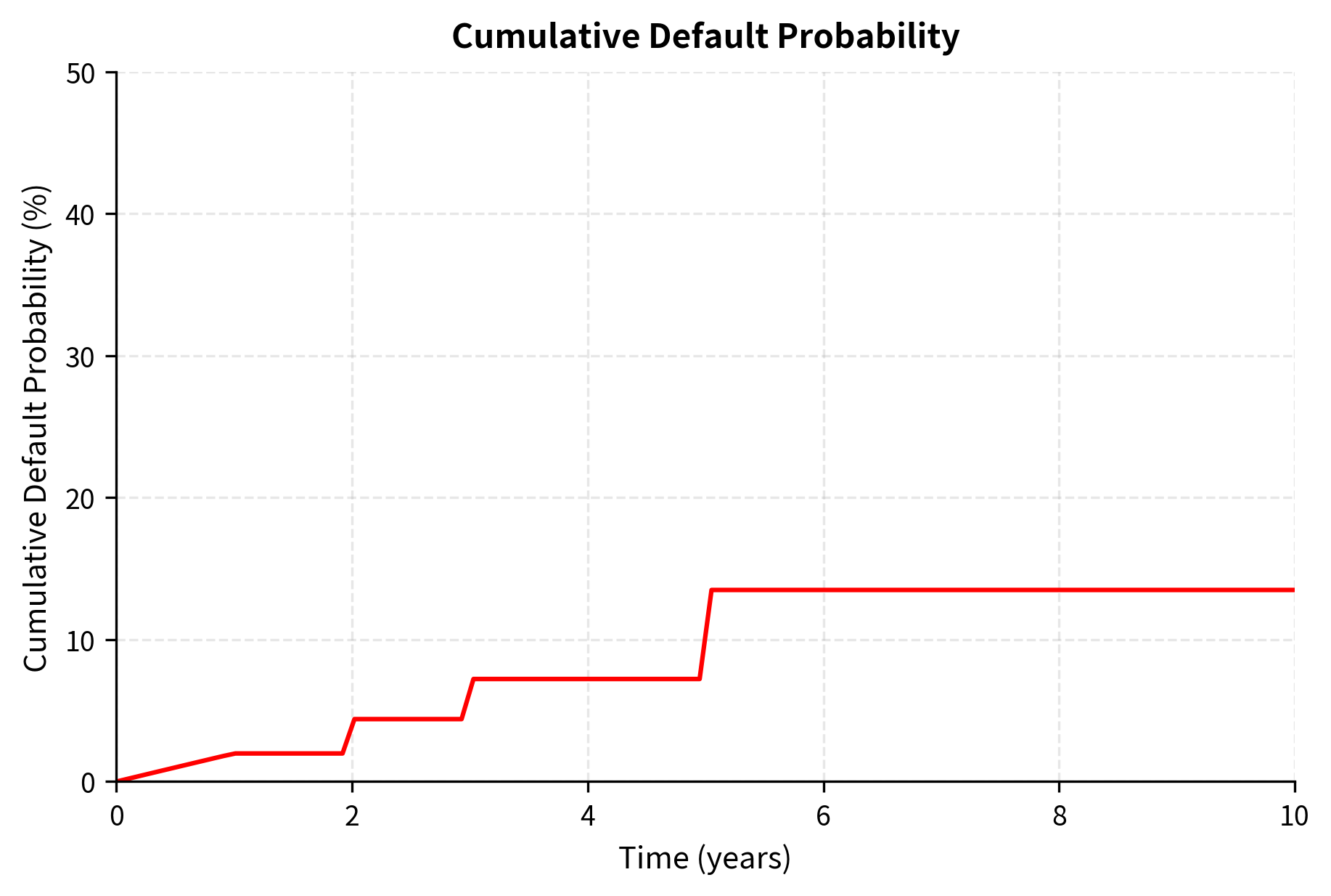
The survival probability declines from 100% to approximately 67% over 10 years, while cumulative default probability rises from 0% to 33%. The upward-sloping hazard rate curve, starting at 2% annually and rising to 4%, reflects the common empirical pattern that credit quality deteriorates over time as uncertainty about the firm's future increases. Short-term default is relatively unlikely because financial distress develops gradually, but as the horizon extends, more scenarios for adverse outcomes become possible. This term structure captures the market's expectation that default risk increases with the time horizon.
Calibrating to CDS Spreads
The primary advantage of reduced-form models is their ability to be calibrated directly to market data. As we discussed in Part II Chapter 13 on credit default swaps, CDS spreads reflect the market's assessment of default risk. The CDS market provides a direct window into market-implied default probabilities, making reduced-form models highly practical for trading and risk management applications.
For a CDS with spread and recovery rate , no-arbitrage pricing requires that the present value of premium payments (premium leg) equals the present value of protection payments (protection leg). This equilibrium condition reflects the fact that a fairly priced CDS has zero initial value: neither party pays upfront because the expected benefits equal the expected costs. This equilibrium allows us to back out the implied hazard rate from observable CDS spreads.
The premium leg represents the periodic payments made by the protection buyer.
where:
- : CDS spread (annualized premium rate paid by protection buyer)
- : number of premium payment periods
- : index for payment periods, running from 1 to
- : length of payment period in years
- : time of the -th payment
- : survival probability to time (premium only paid if no default has occurred)
- : discount factor to time , equal to for continuous discounting
- The sum captures expected present value of all premium payments
The summation reflects that premiums are only paid if the reference entity has not defaulted. Each term multiplies the premium rate by the payment period length, the probability of survival to that date, and the appropriate discount factor. The survival probability weighting is crucial: if default occurs before payment date , that premium is never paid.
where:
- : recovery rate (fraction of notional recovered upon default)
- : loss given default (fraction not recovered)
- : CDS maturity
- : hazard rate (default intensity) at time
- : survival probability to time
- : discount factor for payment at time
- : probability of default occurring in the infinitesimal interval
- The integral sums expected present value of protection payments across all possible default times from 0 to
where is the discount factor to time . The protection leg integral captures the expected payout to the protection buyer. Default can occur at any time between now and maturity, and when it does, the protection seller pays times the notional. The integrand represents the probability density of defaulting at exactly time : the hazard rate times the probability of having survived to that point.
For a flat hazard rate , we can derive an approximate relationship between CDS spread and hazard rate. Under the assumptions that discount rates are small and survival probabilities do not vary too much over the CDS tenor.
Similarly, the protection leg becomes:
Setting these equal (no-arbitrage condition):
Canceling from both sides gives:
where:
- : CDS spread (annualized premium rate)
- : constant hazard rate (default intensity per year)
- : recovery rate
- : loss given default (LGD)
- The approximation holds when discount rates and survival probabilities are relatively stable over the CDS tenor
This relationship shows that CDS spreads compensate for two components of credit risk: the probability of default () and the severity of loss when default occurs (). The approximation becomes increasingly accurate for shorter maturities and lower hazard rates where discounting effects are minimal.
Solving for the hazard rate provides a direct link between observable CDS spreads and default intensity:
where:
- : implied hazard rate (annual default intensity)
- : observed CDS spread
- : assumed recovery rate
- The formula shows that CDS spreads reflect both default risk () and loss severity ()
This simple inversion is remarkably powerful: it allows us to extract market-implied default intensities directly from CDS prices without complex modeling assumptions, making reduced-form models easy to calibrate. The hazard rate interpretation also helps explain why CDS spreads differ across credits: investment-grade companies have low spreads because their hazard rates are low, while distressed companies have high spreads reflecting elevated default intensity.
python #| echo: false #| output: false
import numpy as np
Example: Convert CDS spreads to hazard rates
cds_spreads_bps = np.array([50, 100, 200, 500, 1000]) # Basis points cds_spreads = cds_spreads_bps / 10000 # Convert to decimal recovery = 0.40
hazard_rates_implied = [hazard_rate_from_cds(s, recovery) for s in cds_spreads] annual_default_probs = [1 - np.exp(-h) for h in hazard_rates_implied]
python #| echo: false #| output: true
import pandas as pd import numpy as np
survival_5y = [np.exp(-h*5)*100 for h in hazard_rates_implied]
df = pd.DataFrame({ 'CDS Spread (bps)': cds_spreads_bps, 'Hazard Rate (%)': np.array(hazard_rates_implied) * 100, '1-Year PD (%)': np.array(annual_default_probs) * 100, '5-Year Survival (%)': survival_5y }) print("CDS Spread to Default Probability Mapping (Recovery = 40%)") print("=" * 60) print(df.to_string(index=False, float_format=lambda x: f'{x:.2f}'))
The table reveals the relationship between CDS spreads and default risk across the credit spectrum. A 200 basis point CDS spread implies a hazard rate of 3.33% and annual default probability of 3.27%, with 5-year survival probability of 84.5%. For investment-grade credits (50-100 bps spreads), the mapping is approximately linear because the exponential function is nearly linear for small arguments. However, for distressed credits with spreads of 1000 bps, the hazard rate reaches 16.67% annually, leading to only 43.35% probability of surviving 5 years. At these high spread levels, the approximation becomes less accurate due to the nonlinear relationship between hazard rates and survival probabilities, and practitioners often use more sophisticated models with term structure effects.
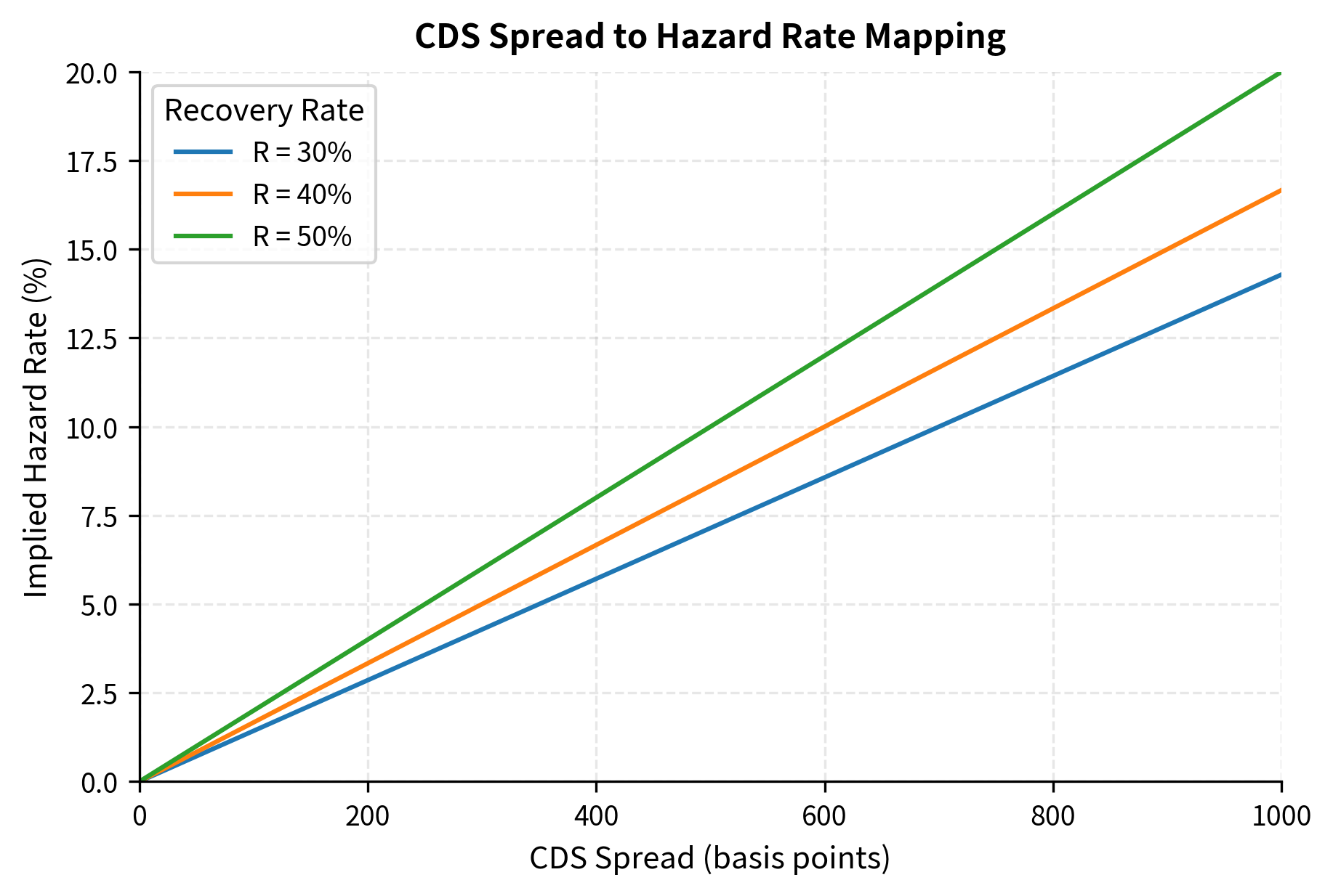
The visualization reveals how recovery rate assumptions affect hazard rate inference. For a given CDS spread, a lower recovery rate implies a lower hazard rate because the expected loss per default is higher. At 500 bps, assuming 30% recovery yields an implied hazard rate of approximately 7.1%, while assuming 50% recovery yields approximately 10%. This sensitivity highlights the importance of accurate recovery rate assumptions when calibrating reduced-form models, as the same CDS spread can imply substantially different default probabilities depending on the assumed recovery.
Stochastic Intensity Models
For more realistic dynamics, the hazard rate itself can be modeled as a stochastic process. Rather than assuming a constant default intensity, we allow it to fluctuate over time in response to changing economic conditions. A firm's credit quality varies with business cycles, competitive pressures, management decisions, and countless other factors. Capturing this time variation requires modeling the hazard rate as a random process.
A common specification is the Cox-Ingersoll-Ross (CIR) process, which ensures the hazard rate remains positive and mean-reverts to a long-term level:
where:
- : hazard rate (default intensity) at time
- : infinitesimal change in the hazard rate over time
- : speed of mean reversion (how quickly returns to its long-term level )
- : long-term mean level of the hazard rate
- : volatility parameter controlling the magnitude of random fluctuations
- : standard Brownian motion driving the random shocks
- : infinitesimal time increment
- : infinitesimal Brownian increment
- : mean reversion term that pulls toward when and pushes it down when
- : square root diffusion term that ensures the hazard rate remains non-negative (volatility scales with the level)
The CIR specification has several desirable properties that make it well-suited for modeling credit risk. The square root diffusion ensures non-negativity: as approaches zero, the volatility shrinks proportionally, making it mathematically impossible for the process to go negative. This is essential since a negative default probability has no economic meaning. The mean reversion term pulls the hazard rate toward its long-term mean , capturing the empirical observation that credit quality tends to revert over economic cycles. When , the drift is positive (credit quality deteriorates toward normal), and when , the drift is negative (credit quality improves from distressed levels). This mean-reverting behavior reflects the idea that extremely good or extremely bad credit conditions are temporary states that tend to normalize over time.
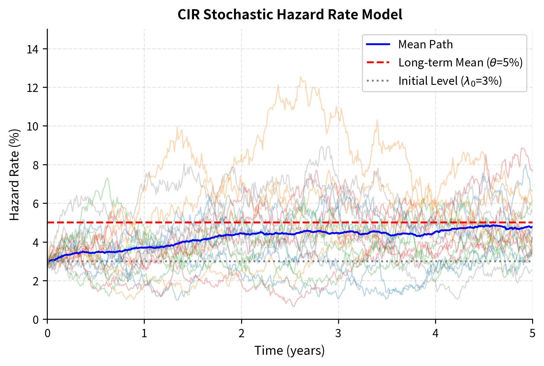
The simulated paths start at 3% hazard rate and exhibit clear mean reversion toward the 5% long-term level specified by theta. Individual paths show substantial volatility, with hazard rates ranging from near 0% to over 12% across scenarios, while the mean path (blue line) converges steadily from the initial 3% toward 5% over the 5-year horizon. The mean reversion speed of 0.5 pulls paths back toward the long-term mean at a moderate rate, preventing extreme persistent deviations while allowing meaningful short-term fluctuations. The fan-like spread of paths illustrates the uncertainty inherent in future credit conditions. This stochastic intensity framework forms the basis for pricing credit derivatives with time-varying default risk, capturing the reality that credit spreads and default probabilities evolve randomly over time.
Credit Scoring and Machine Learning Approaches
While structural and reduced-form models derive from financial theory, credit scoring uses historical data to predict which borrowers will default based on observable characteristics. This approach dominates retail lending (mortgages, credit cards, personal loans) and increasingly complements market-based models for corporate credit. Credit scoring identifies statistical patterns in observable characteristics that distinguish defaulters from non-defaulters. It does not model economic mechanisms like structural approaches.
Logistic Regression for Default Prediction
Logistic regression models the probability of default as a function of borrower characteristics. The model transforms a linear combination of features (financial ratios, firm characteristics) into a probability between 0 and 1 using the logistic function:
where:
- : predicted probability of default (bounded between 0 and 1)
- : number of borrower characteristics (features) in the model
- : borrower characteristic for (e.g., debt-to-equity ratio, profitability, liquidity measures)
- : intercept term (baseline log-odds when all features are zero)
- : coefficient for feature , representing the change in log-odds per unit change in
- : Euler's number (base of natural logarithm, approximately 2.71828)
- : linear combination forming the log-odds or credit score
- The logistic function transforms the unbounded log-odds into a probability between 0 and 1
The linear combination is called the log-odds or credit score. The logistic function, also known as the sigmoid function, transforms this potentially unbounded score into a proper probability.
The logistic function has several attractive properties for classification problems. It is monotonically increasing, so higher scores always correspond to higher default probability, enabling straightforward ranking of borrowers by risk. It asymptotically approaches 0 and 1 at the extremes, ensuring that predictions are always valid probabilities regardless of how extreme the input features become. It has a simple derivative that facilitates maximum likelihood estimation, making parameter fitting computationally tractable even for large datasets. The coefficients have a clear interpretation: each coefficient represents the change in log-odds per unit change in the corresponding feature . A positive coefficient means higher values of that feature increase default probability, while a negative coefficient means higher values decrease default probability.
python #| echo: false #| output: true
from sklearn.metrics import roc_auc_score
print("Logistic Regression Credit Scoring Model") print("=" * 50) print(f"\nModel Performance:") print(f" AUC-ROC Score: {roc_auc_score(y_test, y_pred_proba):.4f}") print(f" Default Rate (Test Set): {y_test.mean():.1%}") print() print("Feature Coefficients (Standardized):") for name, coef in zip(feature_names, logreg.coef_[0]): direction = "↑ risk" if coef > 0 else "↓ risk" print(f" {name:20s}: {coef:+.4f} ({direction})") strong discriminatory power with an AUC-ROC score above 0.85, indicating it effectively separates defaulters from non-defaulters. The coefficients reveal intuitive relationships consistent with financial theory: higher debt-to-equity increases default risk (positive coefficient) because more leverage means less cushion to absorb losses. Better profitability (negative coefficient on profit margin) reduces default risk because profitable firms generate cash to service debt. Stronger liquidity (negative coefficients on current ratio and interest coverage) also reduces default risk because liquid firms can meet short-term obligations. The test set default rate matches the training distribution, suggesting good model calibration without overfitting.
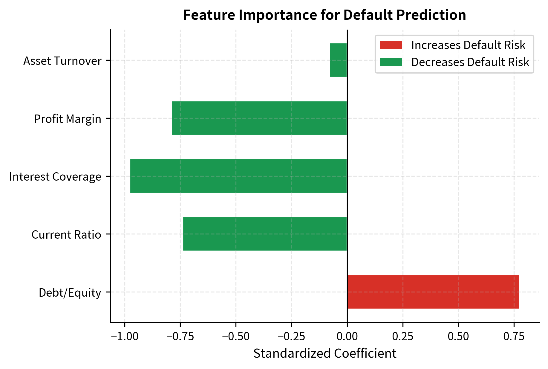
The coefficient visualization provides immediate insight into which factors drive default risk in the model. Debt-to-equity ratio has the largest positive coefficient, indicating high leverage is the strongest predictor of default. All other features have negative coefficients, meaning higher values reduce default probability. Profit margin shows the strongest protective effect: profitable firms generate cash flow to service debt and weather temporary difficulties. The current ratio and interest coverage also contribute materially to lowering predicted default probability, reflecting the importance of liquidity. Asset turnover has a smaller but still negative effect, suggesting operationally efficient firms face lower default risk.
Altman Z-Score: A Classic Scoring Model
Edward Altman's 1968 Z-score remains widely used for bankruptcy prediction. It demonstrates that simple models with clear economic interpretation can be highly effective. The model combines five financial ratios that collectively capture liquidity, profitability, leverage, solvency, and activity. The model combines five financial ratios that collectively capture liquidity, profitability, leverage, solvency, and activity:
where:
- : composite bankruptcy risk score
- : Working Capital / Total Assets (measures liquidity and short-term financial health)
- : Retained Earnings / Total Assets (measures cumulative profitability and firm age)
- : EBIT / Total Assets (measures operating efficiency and profitability before interest and taxes)
- : Market Value of Equity / Book Value of Debt (measures leverage and market confidence in the firm)
- : Sales / Total Assets (measures asset turnover and revenue generation efficiency)
- The coefficients 1.2, 1.4, 3.3, 0.6, and 1.0 were determined empirically through discriminant analysis on historical bankruptcy data
- Higher -scores indicate lower bankruptcy risk, lower scores indicate higher risk
Firms with are classified as distressed, indicating high default risk. Values with indicate healthy firms with low default risk. Values between 1.81 and 2.99 fall in the gray zone where classification is uncertain.
The Z-score's enduring popularity stems from its simplicity and interpretability. Each ratio captures a different dimension of financial health: measures liquidity, the firm's ability to meet short-term obligations. captures cumulative profitability and implicitly firm age, since retained earnings accumulate over time. measures operating performance, the core earnings power of the business before financing decisions. combines market information with book values, capturing both leverage and the market's confidence in the firm's prospects. measures asset efficiency, how effectively the firm uses its assets to generate revenue. The weights reflect their relative importance in predicting bankruptcy, with operating profitability () receiving the highest weight of 3.3, indicating it is the strongest discriminator between healthy and distressed firms.
Company A demonstrates financial health with a Z-score above 3, placing it firmly in the safe zone with low default risk. The strong working capital position indicates liquidity to meet short-term obligations. High retained earnings relative to assets suggest mature profitability and financial stability accumulated over time. Healthy EBIT margins demonstrate operating efficiency, while the favorable ratio of market equity to book debt reflects both low leverage and market confidence in the firm's prospects. In contrast, Company B shows financial distress with a Z-score below 1.81, indicating high default risk. Negative working capital is a serious warning sign, suggesting the firm may struggle to pay current obligations. Weak profitability ratios indicate the core business is not generating adequate returns. High leverage relative to market equity suggests the firm is overleveraged, with debt exceeding what the market believes the equity is worth. These results show how the Z-score effectively synthesizes multiple financial dimensions into a single risk metric. It can be easily communicated and compared across firms.
ROC Analysis and Model Discrimination
The Receiver Operating Characteristic (ROC) curve visualizes how well a credit scoring model separates defaulters from non-defaulters across different probability thresholds. This diagnostic tool is essential for evaluating and comparing credit models.
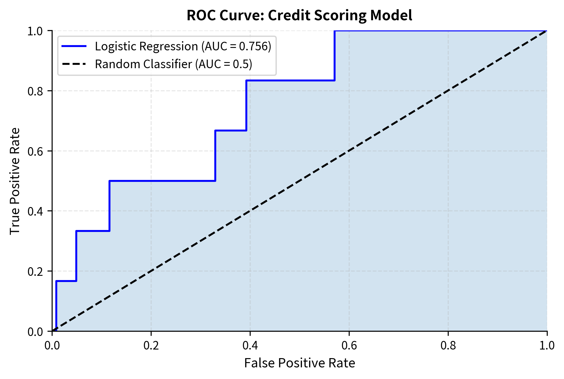
The ROC curve shows strong model performance, with the blue curve rising steeply above the diagonal random classifier line. The diagonal represents a model with no discriminatory power: one that assigns default probabilities randomly and thus performs no better than chance. The area under the ROC curve (AUC) quantifies overall discriminatory power. An AUC of 0.5 represents random guessing, while 1.0 represents perfect discrimination where all defaulters are assigned higher risk scores than all non-defaulters. The logistic regression model achieves an AUC above 0.85, placing it in the upper range of typical credit scoring models (0.70-0.85). This level of discriminatory power meets most regulatory requirements for internal risk models and indicates the model effectively ranks borrowers by risk. The curve also reveals the tradeoff faced at any threshold: moving left along the curve reduces false positives (healthy firms incorrectly flagged) but also reduces true positives (actual defaults caught).
Portfolio Credit Risk Models
Individual default probabilities tell only part of the story of portfolio risk. When managing a portfolio of loans or bonds, the key risk driver is default correlation: the tendency for multiple obligors to default together. A portfolio of 1,000 independent loans with 1% default probability each has predictable losses around the mean, with the law of large numbers ensuring relatively modest deviations. But if defaults are correlated, as during economic downturns, the portfolio can experience catastrophic losses far exceeding expectations. Understanding and modeling this correlation is the central challenge of portfolio credit risk management.
Default Correlation and Joint Default Probability
Consider two obligors with individual default probabilities and . If defaults were independent, the joint probability would simply be the product . But in reality, defaults are positively correlated, economic conditions that cause one firm to default often affect others as well. Under the Gaussian copula framework, we model each obligor's creditworthiness through a latent variable that follows a standard normal distribution. This latent variable can be thought of as an abstract measure of the firm's financial health, with lower values indicating worse conditions. Obligor defaults when this latent variable falls below the threshold .
When the two latent variables have correlation , we can calculate the joint default probability using the bivariate normal distribution. The probability that both obligors default is the probability that both latent variables simultaneously fall below their respective thresholds:
where:
- : probability that both obligors 1 and 2 default
- : individual default probabilities for obligors 1 and 2
- : correlation coefficient between the latent variables driving defaults (ranges from -1 to 1)
- : inverse of the cumulative standard normal distribution function
- : standard normal threshold corresponding to default probability (the critical value below which default occurs)
- : bivariate standard normal cumulative distribution function, giving when and are correlated standard normals with correlation
- This Gaussian copula approach elegantly separates marginal behavior (individual default probabilities) from dependence structure (correlation)
The copula approach gains its flexibility from this separation of concerns. The marginal default probabilities can be estimated or calibrated independently for each obligor using any method (structural models, credit scores, historical data). The copula then combines these marginals with a dependence structure specified by the correlation parameter. This modularity makes the framework highly flexible and practical for large portfolios with heterogeneous obligors.
Correlation dramatically increases joint default probability, far beyond what intuition might suggest. Under independence (ρ=0), the joint probability equals the product of individual probabilities at 0.04%, representing the case where each firm's fate is determined by entirely separate factors. However, at 50% correlation, joint default probability rises to approximately 0.15%, nearly 4 times the independent level. At 70% correlation, the multiplier exceeds 7x. This superlinear increase in joint default risk with correlation illustrates the concentration risk inherent in portfolios of correlated credits, making portfolio credit modeling essential for risk management. The economic interpretation is clear: when times are bad, they tend to be bad for many firms simultaneously, creating clustering of defaults that can devastate portfolios.
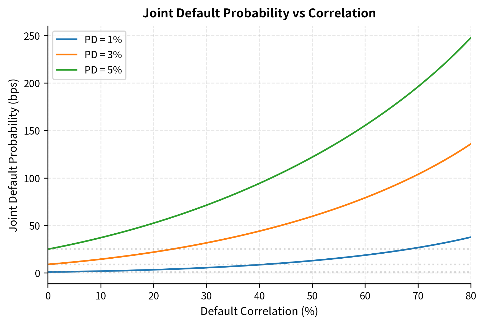
The figure illustrates how joint default probability increases with correlation across different credit quality levels. For investment-grade obligors with 1% PD, the joint default probability under independence is just 1 basis point (0.01%), but rises to approximately 30 bps at 70% correlation. For speculative-grade obligors with 5% PD, the increase is even more dramatic: from 25 bps under independence to over 200 bps at high correlation. The dotted horizontal lines show the independent joint probability for reference, highlighting how correlation can multiply joint default risk by factors of 10x or more. This visualization shows why correlation is critical for portfolio credit risk.
The Gaussian Copula Model
The Gaussian copula framework, widely used before the 2008 crisis for CDO pricing (as discussed in Part II Chapter 14), models defaults through a latent factor structure. The key insight is that defaults across a portfolio can be driven by both common factors affecting all firms, and idiosyncratic factors unique to each firm. Each obligor's creditworthiness depends on both systematic (economy-wide) and idiosyncratic (firm-specific) factors:
where:
- : latent "asset return" variable driving obligor 's default (higher values indicate better creditworthiness)
- : index for the obligor
- : common systematic factor representing economy-wide conditions (e.g., GDP growth, market returns), with
- : obligor 's idiosyncratic factor representing firm-specific risk independent of other obligors, with
- : correlation coefficient between obligor 's asset return and the systematic factor (determines systematic risk exposure, ranges from 0 to 1)
- : weight on the systematic factor
- : weight on the idiosyncratic factor
- The weights ensure has unit variance when and are independent standard normal random variables
- Since and are independent standard normals, is also standard normal:
Obligor defaults if , where is their individual default probability. The threshold is chosen so that the unconditional default probability matches the calibrated value for each obligor.
Default Correlation Mechanism
The factor structure elegantly captures how default correlation emerges from exposure to common economic conditions. When the systematic factor is low (representing an economic downturn), all obligors' values decrease simultaneously by , increasing the probability that multiple firms cross their default thresholds together. The correlation parameter controls this sensitivity: obligors with high ρ_i are strongly affected by systematic conditions and thus highly correlated with each other, while obligors with low are driven primarily by idiosyncratic factors and have weak correlation with others.
This single-factor structure explains why defaults cluster during recessions even among apparently unrelated firms. A retailer and a manufacturer in different industries may seem independent, yet both are affected by consumer confidence, credit availability, and overall economic growth. The systematic factor captures these common influences. During normal times, the idiosyncratic factors dominate and defaults appear somewhat random. But during severe recessions when takes extreme negative values, the systematic component pushes many firms toward their default thresholds simultaneously, creating the default clustering that devastates credit portfolios.
output: true
import numpy as np
total_exposure = np.sum(exposures) avg_pd = np.mean(default_probs) avg_corr = np.mean(correlations) exp_loss = results['expected_loss'] var_val = results['var'] unexp_loss = results['unexpected_loss'] var_el_ratio = var_val / exp_loss
print("Portfolio Credit Risk Analysis (Gaussian Copula Model)") print("=" * 55) print(f"Number of Obligors: {n_obligors}") print(f"Total Exposure: {total_exposure/1e6:.1f} million") print(f"Average PD: {avg_pd:.2%}") print(f"Average Correlation: {avg_corr:.1%}") print() print("Risk Metrics:") print(f" Expected Loss: {exp_loss/1e6:.2f} million ({exp_loss/total_exposure:.2%} of exposure)") print(f" 99% Credit VaR: {var_val/1e6:.2f} million ({var_val/total_exposure:.2%} of exposure)") print(f" Unexpected Loss: {unexp_loss/1e6:.2f} million") print(f" VaR/EL Ratio: {var_el_ratio:.1f}x")
The portfolio exhibits moderate credit risk with expected loss reflecting the average default probability and loss given default assumptions. Expected loss represents the actuarial cost of credit risk, the average loss that would be experienced over many repetitions of the same portfolio. However, the 99% Credit VaR reveals significant tail risk in adverse scenarios. The VaR/EL ratio measures how much worse losses can get beyond expectations. The calculated ratio is typical for diversified portfolios, but concentrated or highly correlated portfolios can have much higher ratios. The unexpected loss component, the difference between VaR and expected loss, represents the buffer needed to absorb losses in stress scenarios. This is the capital that must be held to remain solvent with 99% confidence.
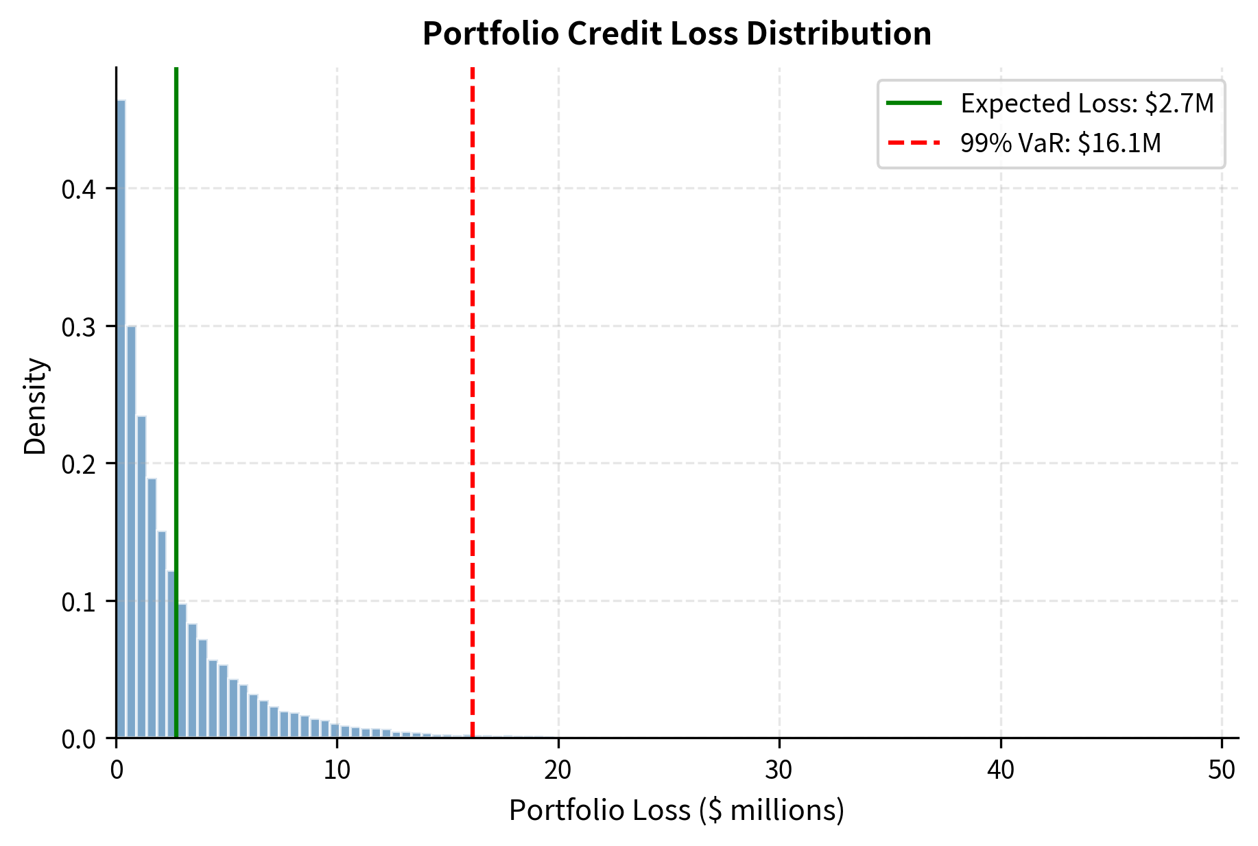
The loss distribution exhibits the characteristic positive skew of credit portfolios. Most simulated scenarios produce losses near the expected value, clustering around the peak of the distribution. But the fat right tail extends significantly beyond, reflecting scenarios where many defaults coincide. The 99% VaR substantially exceeds the expected loss, illustrating that tail risk significantly exceeds typical outcomes. This asymmetry arises because losses are bounded below at zero (you cannot have negative credit losses) but unbounded above when multiple defaults coincide. Extreme losses, while rare (occurring in only 1% of scenarios), can be many times larger than the expected loss. This tail risk is the primary concern for risk managers and regulators because it represents scenarios that can threaten portfolio solvency or even institutional failure.
Correlation Sensitivity
Default correlation is the key driver of portfolio tail risk. Let's examine how correlation affects the loss distribution to develop intuition for this critical relationship:
Quiz
Ready to test your understanding? Take this quick quiz to reinforce what you've learned about credit risk modeling approaches.

Comments