Credit Risk Fundamentals: PD, LGD, and EAD Framework

Credit risk is the possibility of financial loss arising from a borrower's failure to repay a loan or meet contractual obligations. While market risk, which we examined in the previous chapter, stems from movements in prices, rates, and volatilities, credit risk arises from the potential deterioration or default of a counterparty's creditworthiness. For banks, insurance companies, and asset managers, credit risk often represents the largest source of potential losses. Understanding and quantifying this risk is essential for pricing loans, setting aside reserves, and making sound investment decisions.

The 2008 financial crisis showed the dangers of poorly understood and mispriced credit risk. Subprime mortgage defaults cascaded through structured credit products, amplified by interconnected counterparty exposures, ultimately threatening the global financial system. What began as localized losses in one segment of the housing market quickly spread into a systemic crisis, showing how deeply credit risk affects modern financial markets. This crisis showed why rigorous credit risk measurement is essential and led to reforms that still shape the industry today.

This chapter introduces the foundational framework for quantifying credit risk through three key components: the Probability of Default (PD), Loss Given Default (LGD), and Exposure at Default (EAD). Together, these parameters allow us to calculate expected losses and inform decisions about loan pricing, bond valuation, capital allocation, and loss provisioning. Building on our earlier discussion of credit default swaps and structured credit products in Part II, we now examine the quantitative mechanics underlying credit risk assessment. By the end of this chapter, you will understand not just the formulas themselves, but the intuition behind each component and how they work together to provide a complete picture of credit risk.

Credit risk manifests in several forms, each requiring your careful attention. Default risk is the most severe form: a borrower fails to make required payments, triggering legal remedies and potential losses for creditors. This is the ultimate credit event that the entire framework is designed to assess. Credit migration risk occurs when a borrower's credit quality deteriorates, increasing the likelihood of future default and reducing the value of existing exposures. Even without an actual default, a downgrade from investment grade to speculative grade can cause significant mark-to-market losses for bondholders. Spread risk, which we touched on when discussing CDS pricing, reflects changes in credit spreads even without actual default or rating changes. These spread movements reflect the market's evolving assessment of creditworthiness and can create substantial gains or losses for holders of credit-sensitive instruments.

The fundamental equation of credit risk measurement combines three components into a single expression for expected credit losses:

where:

• $\text{Expected Loss}$: the average loss anticipated over the time horizon
• $\text{PD}$: Probability of Default, the likelihood that the borrower will default within a given time horizon
• $\text{LGD}$: Loss Given Default, the fraction of exposure lost if default occurs
• $\text{EAD}$: Exposure at Default, the amount owed at the moment of default

This deceptively simple formula answers three core questions. First, how likely is it that this borrower will fail to meet their obligations? Second, if they do default, how much of our exposure will we actually lose after recovery efforts? Third, at the moment of default, how much will we have at stake? This framework is modular: each component can be analyzed, estimated, and modeled separately, yet they combine to produce a single, actionable measure of expected credit loss.

Each component requires careful estimation and carries its own sources of uncertainty. Probability of Default depends on the borrower's financial health, industry conditions, and macroeconomic factors. Loss Given Default varies with collateral quality, seniority in the capital structure, and the economic environment at the time of default. Exposure at Default can change over time as borrowers draw on credit lines or as derivative exposures fluctuate with market conditions. We'll examine each in depth before bringing them together to see how the complete framework operates in practice.

Probability of Default (PD) is the chance a borrower fails to meet debt obligations, usually within a year. It is a widely studied part of credit risk because it predicts uncertain future events. Estimating PD uses historical data, fundamental analysis, and market signals. Different approaches offer different perspectives on creditworthiness, and you often use multiple methods to estimate default risk.

Credit rating agencies, such as Moody's, Standard & Poor's, and Fitch, provide independent assessments of creditworthiness that have become a cornerstone of global fixed income markets. These grades provide a common way to describe credit quality and compare borrowers. These ratings carry significant implications: they influence bond yields, determine eligibility for investment mandates, and trigger collateral requirements in derivative contracts. The letter grades translate into broad categories of default probability based on decades of observed default experience:

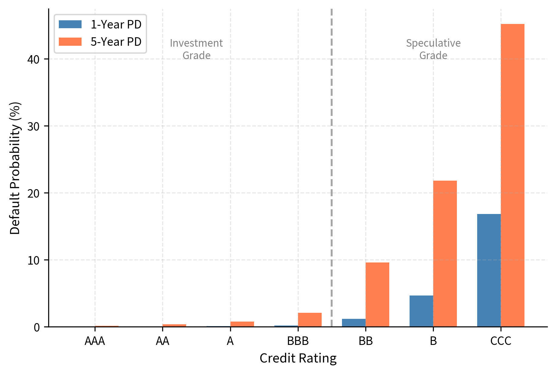
The table reveals the dramatic increase in default probability as ratings decline, a pattern that demonstrates the informational content embedded in credit ratings. An investment-grade BBB-rated company has roughly a 0.18% annual default probability, while a B-rated speculative company faces a 4.65% chance of defaulting within a year, which is about 26 times higher. This exponential increase in default risk as ratings deteriorate explains why the boundary between investment grade (BBB and above) and speculative grade (BB and below) carries such significance in financial markets. Many institutional investors face restrictions on holding speculative-grade debt, and the crossing of this threshold can trigger forced selling that further depresses bond prices.

Rating agencies develop their assessments through qualitative and quantitative analysis of business risk (industry dynamics, competitive position, management quality) and financial risk (leverage, interest coverage, cash flow stability). Analysts examine a company's strategic positioning, its ability to generate consistent cash flows, and its capacity to service debt obligations under adverse conditions. While ratings provide useful benchmarks, they have limitations: they're typically "through-the-cycle" assessments designed to be stable over time, which means they may not capture rapidly changing credit conditions. This stability is intentional, as it prevents excessive rating volatility that could disrupt markets, but it also means ratings can lag behind deteriorating fundamentals until the problems become severe.

As we discussed in our coverage of credit default swaps, market prices embed information about perceived default risk that updates continuously with market conditions. The CDS spread reflects the premium investors demand for bearing default risk, allowing us to extract an implied probability of default directly from observable market prices. This market-based approach provides a valuable complement to rating agency assessments, offering a real-time view of how the market perceives creditworthiness.

For a simplified calculation, we can approximate the risk-neutral PD from CDS spreads. The intuition is that the CDS spread (insurance premium) must compensate the seller for the expected loss, which is the product of the default probability and the loss severity ($1 - \text{Recovery Rate}$). Think of it this way: if you are selling insurance against default, you need to charge a premium that at least covers the expected payout. The expected payout equals the probability of having to pay out multiplied by the amount you would lose. We can derive the implied PD by equating the CDS spread to the expected loss rate and solving for the unknown default probability:

where:

• $\text{PD}_{\text{implied}}$: implied probability of default derived from market prices
• $\text{CDS Spread}$: cost of credit protection (expressed as a decimal)
• $\text{Recovery Rate}$: expected fraction of exposure recovered in default

The key parameters for the market-implied PD calculation are:

• CDS Spread: The annual cost of credit protection in basis points. Higher spreads imply higher default risk.
• Recovery Rate: The fraction of exposure expected to be recovered in default. Lower recovery rates imply lower default probabilities for a given spread.
• Time Horizon: The period over which the default probability is estimated.

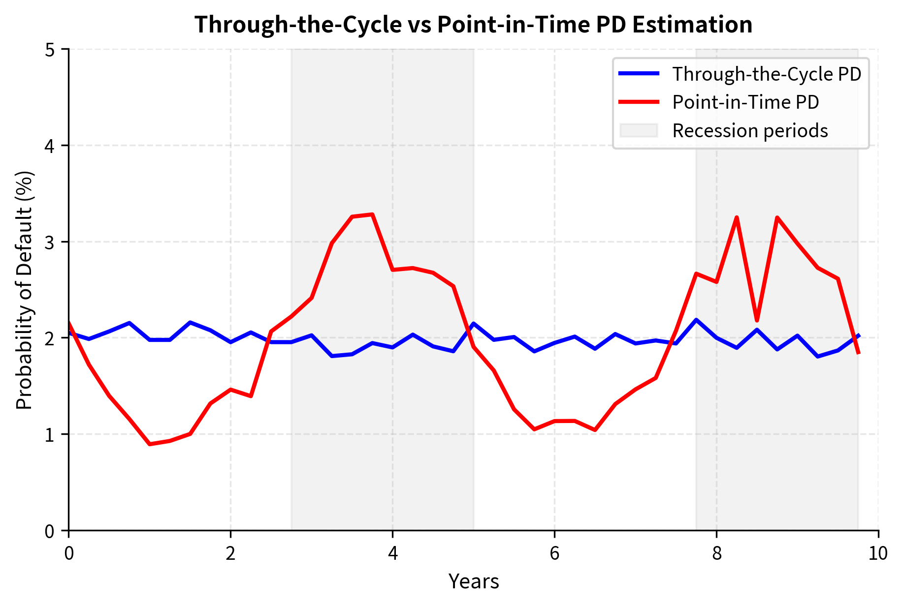
A crucial distinction in PD estimation is between through-the-cycle (TTC) and point-in-time (PIT) approaches, which represent fundamentally different philosophies about how to assess credit risk. Understanding this distinction is essential for interpreting PD estimates correctly and choosing the right approach for each application.

The difference between these approaches has profound practical implications. A TTC assessment asks: "What is the average default probability for this type of borrower across good times and bad?" A PIT assessment asks: "Given what we know about current economic conditions and this specific borrower's current situation, what is the default probability right now?" Both questions are valid, but they serve different purposes.

The choice between TTC and PIT depends on the application. For pricing loans at origination, TTC PD provides stability and ensures consistent treatment of similar borrowers regardless of where we are in the economic cycle. This prevents the procyclical lending behavior where banks extend too much credit during booms (when PIT PDs are low) and restrict credit excessively during downturns (when PIT PDs spike). For calculating accounting provisions or short-term risk management, PIT PD better reflects current conditions and provides a more accurate estimate of near-term expected losses. Basel regulatory frameworks have moved toward PIT estimates for expected credit loss calculations, recognizing that provisions should reflect the best current estimate of losses rather than long-term averages.

Beyond statistical approaches based on historical default rates or market prices, structural models derived from option pricing theory provide a theoretically grounded framework for PD estimation. These models start from first principles about what causes default and derive default probabilities from observable financial variables. The Merton model, which we'll explore more fully in the next chapter, treats equity as a call option on the firm's assets. Default occurs when asset value falls below the debt's face value at maturity, triggering bankruptcy.

The key insight is that a firm's equity holders have limited liability: if assets fall below debt obligations, they can "put" the firm to creditors and walk away. From the shareholders' perspective, they have the right, but not the obligation, to pay off the debt and keep any residual value. This is precisely the payoff structure of a call option, where the asset value is the underlying and the debt face value is the strike price. This optionality allows us to use option pricing techniques to estimate default probability. Assuming the firm's asset value follows a log-normal distribution (as in the Black-Scholes framework), the probability of default is the probability that the asset value $V$ falls below the debt face value $D$ at maturity $T$:

where:

• $\text{PD}$: probability of default
• $d_2 = \frac{\ln(V/D) + (\mu - \frac{1}{2}\sigma_V^2)T}{\sigma_V\sqrt{T}}$: distance to default, measuring how many standard deviations the asset value is from the debt face value
• $V$: current asset value
• $D$: face value of debt
• $\mu$: expected asset return
• $\sigma_V$: asset volatility
• $T$: time to maturity
• $N(\cdot)$: cumulative standard normal distribution function

The $d_2$ term, often called the "distance to default," provides an intuitive measure of credit quality. It represents, in standardized units, how far the firm's assets must fall before default becomes inevitable. A higher distance to default indicates a safer credit, while a lower or negative distance to default signals imminent distress. This structural approach has the advantage of linking default probability directly to observable firm characteristics like leverage and asset volatility, providing economic intuition for why certain firms are riskier than others.

When default occurs, creditors rarely lose their entire exposure. Recovery comes through liquidation of assets, restructuring agreements, or bankruptcy proceedings. Bankruptcy processes aim to maximize creditor value, often through reorganization or liquidation. Loss Given Default (LGD) is the percentage of exposure not recovered after default:

where:

• $\text{LGD}$: Loss Given Default, representing the percentage of exposure lost
• $\text{Recovery Rate}$: percentage of exposure recovered through liquidation or restructuring

Estimating LGD is equivalent to estimating recovery rates. Both perspectives are useful. When thinking about what drives losses, the LGD framing is natural. When analyzing bankruptcy outcomes and workout processes, the recovery rate perspective may be more intuitive. The challenge lies in predicting, at the time of loan origination, what recovery rate will ultimately be realized years later under uncertain circumstances.

Recovery rates vary significantly based on several factors, and understanding these drivers is essential for accurate LGD estimation. Let's look at the main factors.

Seniority in the capital structure determines the priority of claims in bankruptcy. The capital structure is essentially a queue: when assets are liquidated, senior secured debt holders are paid first, followed by senior unsecured, subordinated, and finally equity holders. This priority ordering is legally enforced through bankruptcy proceedings and significantly affects expected recoveries. A senior secured lender may recover most or all of their claim, while junior creditors may receive only pennies on the dollar.

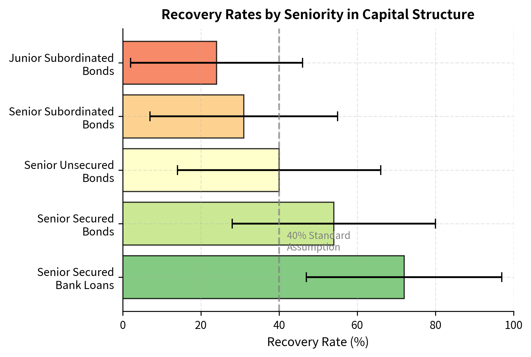
The data shows a clear hierarchy of claims that reflects the legal priority structure: senior secured loans recover roughly 72% of their value, while junior subordinated bonds recover only 24%. This spread illustrates how capital structure priority directly impacts credit losses. The difference of nearly 50 percentage points in recovery rates translates directly into LGD estimates and, consequently, into dramatically different expected losses for lenders at different positions in the capital structure. This is why seniority is one of the most important factors in loan pricing and why senior secured lending commands lower spreads than unsecured or subordinated lending.

Collateral and security significantly affect recovery. Secured loans backed by specific assets (equipment, real estate, receivables) typically achieve higher recoveries than unsecured obligations because the lender has a direct claim on identifiable assets that can be seized and sold. The quality and liquidity of collateral matters enormously: marketable securities or prime real estate can be sold quickly at near-market prices, while specialized industrial equipment may fetch lower prices in distress as potential buyers are limited. You must carefully evaluate not just the current value of collateral, but its likely liquidation value under stressed conditions.

Industry and economic conditions at the time of default influence recovery rates in ways that create unfortunate correlations. During systemic crises, when many firms default simultaneously, asset values are depressed and recoveries tend to be lower. If numerous steel companies default at once, the market for used steel equipment becomes glutted, driving down liquidation values. Industries with tangible assets (utilities, telecommunications) generally see better recoveries than those with primarily intangible assets (technology, services), where the value resides in intellectual property, brand names, and human capital that may evaporate in bankruptcy.

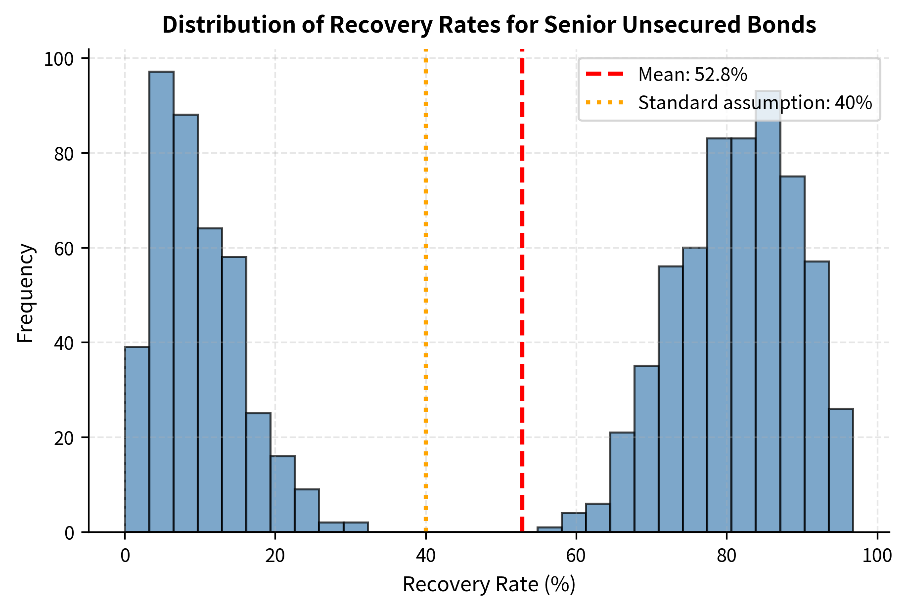
The distribution of recovery rates is notably non-normal, often exhibiting bimodality; defaults either result in near-total loss or substantial recovery, with fewer outcomes in between. This pattern emerges because some defaults involve fundamentally unviable businesses where asset values collapse, while others represent temporary liquidity problems in otherwise sound enterprises that can be successfully restructured. This characteristic makes LGD estimation challenging and suggests that using a single point estimate like 40% oversimplifies the true risk. The wide standard deviation around mean recovery rates implies substantial uncertainty in any individual LGD estimate, which must be accounted for in risk management.

Regulators require banks to consider "downturn LGD" (recovery rates during stressed economic conditions) for capital calculations. Historical evidence shows that recoveries decline precisely when default rates spike, creating an unfortunate correlation that amplifies credit losses during crises. This phenomenon represents one of the most challenging aspects of credit risk: the parameters that determine losses are not independent but move together in adverse ways during stressed periods.

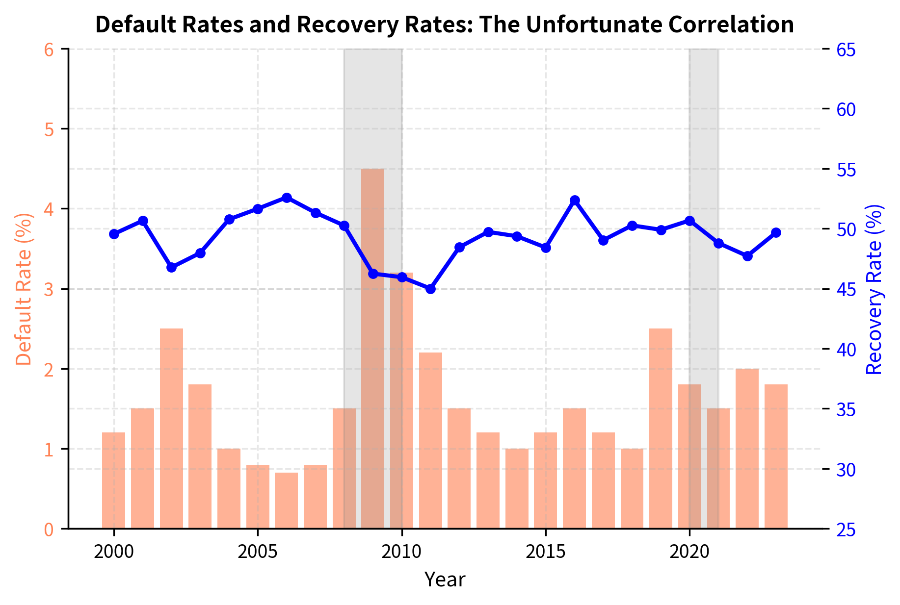
The inverse relationship between default rates and recovery rates creates a double whammy for creditors during downturns. Not only do more borrowers default, but each default results in larger losses. This correlation arises from common underlying factors: economic recessions depress both corporate profitability (increasing defaults) and asset values (reducing recoveries). Understanding and modeling this correlation is essential for stress testing and capital planning, as it means that average-cycle estimates of LGD may significantly understate losses during the periods that matter most.

Exposure at Default (EAD) is the amount a borrower owes when they default. It determines the scale of potential loss; even with zero recovery, losses are limited to the exposure. For a standard term loan, EAD might seem straightforward: simply the outstanding principal plus accrued interest. However, EAD becomes more complex for revolving facilities, commitments, and derivative exposures, where the amount at risk can change significantly between now and the time of default.

For drawn loans, EAD equals the current outstanding balance, a simple and observable quantity:

where:

• $\text{EAD}_{\text{drawn}}$: Exposure at Default for fully funded loans
• $\text{Outstanding Principal}$: current unpaid principal balance
• $\text{Accrued Interest}$: interest earned but not yet paid

For undrawn commitments (credit lines), you must estimate how much the borrower will draw before defaulting. This introduces behavioral uncertainty: will a distressed borrower tap their available credit lines? Historically, borrowers in distress tend to draw down available credit lines aggressively, using every available source of liquidity in an attempt to survive. This means assuming zero utilization would significantly underestimate EAD. The Credit Conversion Factor (CCF) captures this behavior by estimating what portion of unused credit lines will typically be drawn before default occurs:

where:

• $\text{EAD}_{\text{commitment}}$: Exposure at Default for a facility with undrawn capacity
• $\text{Drawn Amount}$: currently utilized portion of the credit line
• $\text{CCF}$: Credit Conversion Factor, estimating the percentage of undrawn line that will be drawn before default
• $\text{Undrawn Amount}$: available but unutilized credit limit

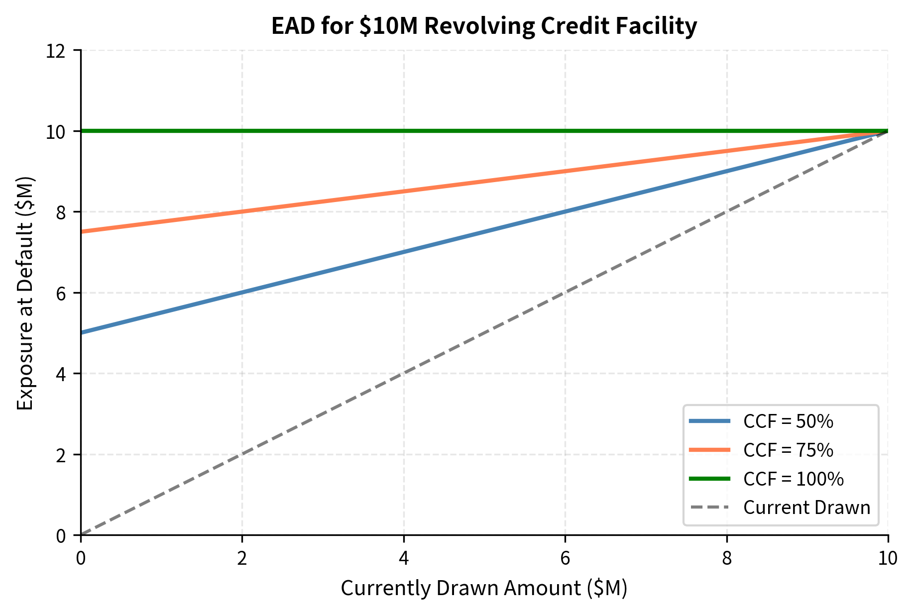
The calculated EAD of $8.25 million reflects the likelihood that a distressed borrower will utilize remaining liquidity. This is significantly higher than the current $3 million balance, showing why credit line exposures require careful EAD estimation.

Basel regulations specify minimum CCF values depending on facility type and commitment characteristics. Unconditionally cancellable commitments (like credit cards where the issuer can reduce the limit at any time) may have lower CCFs than committed facilities where you cannot withdraw the credit line. The rationale is that if you can cancel the commitment when you detect deterioration, the borrower has less opportunity to draw before default.

For derivative contracts, exposure is not simply the notional amount but rather the potential positive value the contract could have at default. As we discussed when covering forwards and swaps, a derivative has both a current mark-to-market value and future uncertainty about how that value might evolve. This makes derivative EAD more complex than loan EAD, as it depends on market movements between now and the potential default date.

The Basel framework defines two components for derivative EAD that together capture both the current exposure and the potential for that exposure to increase:

where:

• $\text{EAD}_{\text{derivative}}$: Exposure at Default for a derivative contract
• $\text{Current Exposure}$: replacement cost today (max of 0 or mark-to-market value)
• $\text{Add-on for Potential Future Exposure}$: estimate of potential increase in value over the risk horizon

The current exposure equals the positive mark-to-market value (if the counterparty owes us money). If the derivative is out of the money from our perspective, meaning we owe the counterparty, the current exposure is zero since their default would not cause us a loss on this position. The add-on captures how much that exposure could grow before we could close out the position after default. This add-on depends on the volatility of the underlying risk factor and the time remaining until the position could be replaced.

The EAD of $1.70 million is significantly higher than the current $1.20 million mark-to-market value, reflecting the risk that interest rates could move further in your favor before a default occurs. This conservatism is intentional: if our counterparty defaults when they owe us the most, that's precisely when our exposure matters.

Netting agreements and collateral arrangements significantly reduce derivative EAD. When parties have multiple trades under an ISDA master agreement with netting provisions, exposure is calculated on a net basis rather than summing gross positive values. If we have ten swaps with a counterparty, some in our favor and some against us, netting allows us to offset these positions, dramatically reducing credit exposure. We'll explore counterparty credit risk and these mitigation techniques more deeply in an upcoming chapter.

The key parameters for Exposure at Default calculations are:

• Commitment Size: The total credit limit available to the borrower.
• Drawn Amount: The portion of the credit line currently utilized.
• CCF (Credit Conversion Factor): The percentage of the undrawn commitment expected to be drawn before default.
• Mark-to-Market: The current replacement cost of a derivative contract.
• Notional Amount: The reference amount used to calculate payments, driving potential future exposure.
• Maturity: Time remaining in the contract. Longer maturities typically attract higher add-on factors for potential future exposure.

With all three components defined, we can calculate expected loss by multiplying them together:

where:

• $\text{EL}$: Expected Loss in currency units
• $\text{PD}$: Probability of Default
• $\text{LGD}$: Loss Given Default (%)
• $\text{EAD}$: Exposure at Default (currency units)

This formula represents the average loss we expect over the time horizon, considering the probability-weighted outcome. To understand why this multiplication makes sense, think of it as a weighted average. With probability PD, default occurs and we lose LGD percent of our EAD exposure. With probability (1 - PD), no default occurs and we lose nothing. The expected value calculation yields EL = PD × LGD × EAD + (1 - PD) × 0 = PD × LGD × EAD. This simple yet powerful formula serves as the foundation for loan pricing, provisioning, and understanding the credit risk contribution of individual exposures.

The expected loss calculation reveals that the B-rated Company D, despite having the smallest exposure, contributes disproportionately to portfolio expected loss due to its high PD. At 4.65% annual default probability and 60% LGD, Company D's $2 million exposure generates $55,800 in expected loss, more than twice the expected loss from Company B's exposure that is five times larger. This insight informs risk-based pricing: higher-risk borrowers should pay higher spreads to compensate for expected losses. Without this differentiated pricing, the portfolio would effectively subsidize risky borrowers at the expense of safer ones.

Expected loss directly informs credit spread requirements. You must charge enough to cover expected losses plus a return for unexpected losses and administrative costs. If spreads are set below this minimum, the lending business destroys value; if set above, you earn economic profit:

where:

• $\text{Credit Spread}$: yield spread charged to the borrower
• $\text{EL Rate}$: Expected Loss expressed as an annualized percentage
• $\text{Unexpected Loss Premium}$: compensation for capital held against tail risk
• $\text{Operating Costs}$: administrative expenses and overhead

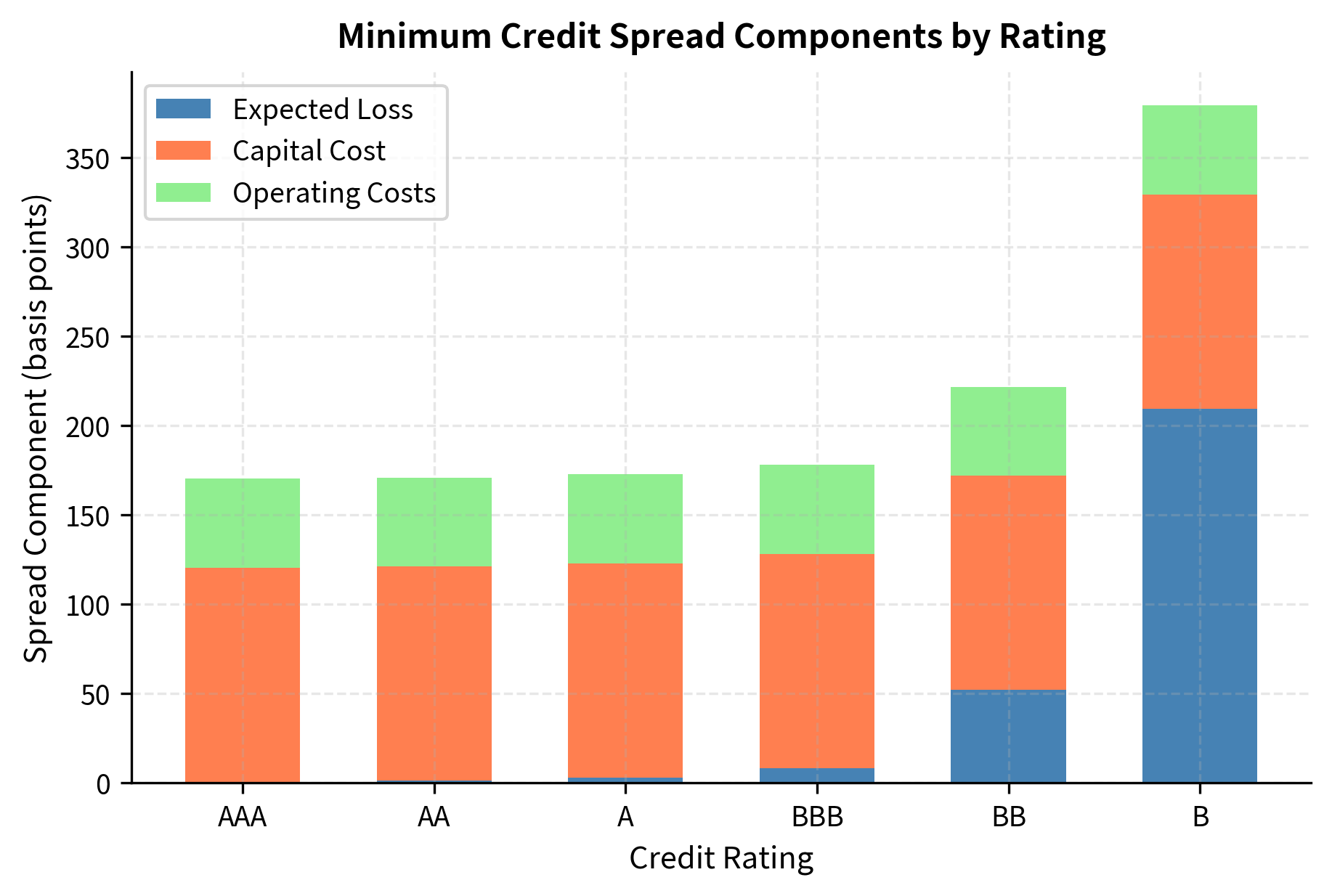
This framework explains why credit spreads exceed simple expected loss rates by a substantial margin. The expected loss for a BBB borrower is only about 8 basis points, yet the minimum viable spread is approximately 178 basis points. The capital cost component, which ensures shareholders earn an adequate return on the capital held against potential unexpected losses, dominates the pricing. This capital must be held to absorb losses that exceed expectations, and shareholders require compensation for putting that capital at risk.

While expected loss represents the mean outcome, credit risk management also requires understanding the potential for losses exceeding expectations. Expected loss tells us the average, but risk management is fundamentally concerned with tail outcomes. Unexpected loss captures the volatility around expected loss, providing a measure of how much actual losses might deviate from the average:

where:

• $\text{UL}$: Unexpected Loss (one standard deviation of the loss distribution)
• $\text{Var}(\text{Loss})$: variance of the credit loss
• $\text{EAD}$: Exposure at Default
• $\text{PD}$: Probability of Default
• $\text{LGD}$: Expected Loss Given Default
• $\text{Var}(\text{LGD})$: variance of the Loss Given Default parameter
• $\text{PD} \times (1-\text{PD}) \times \text{LGD}^2$: component of variance due to uncertainty in the default event itself
• $\text{PD} \times \text{Var}(\text{LGD})$: component of variance due to uncertainty in the recovery rate given default occurs

The formula decomposes variance into two sources. The first term captures uncertainty about whether default will occur: this is the variance of a Bernoulli random variable with probability PD, multiplied by the squared loss severity. The second term captures uncertainty about the severity of loss given that default does occur, reflecting the variability in recovery outcomes. Both sources of uncertainty contribute to unexpected loss and must be managed.

For a portfolio, we must also consider default correlation, which is the tendency for defaults to cluster during economic downturns. When the economy weakens, many borrowers experience stress simultaneously, leading to higher-than-expected default rates precisely when the portfolio is most vulnerable. The unexpected loss of a portfolio is determined by the covariance between individual exposures:

where:

• $\text{UL}_{\text{portfolio}}$: Unexpected Loss of the portfolio
• $\text{UL}_i$: Unexpected Loss of individual loan $i$
• $\rho_{ij}$: correlation of losses (or defaults) between loan $i$ and loan $j$

The second term captures the correlation effect, and its importance cannot be overstated. If correlations are zero, the portfolio UL is simply the square root of the sum of squared individual ULs, meaning diversification works perfectly and portfolio risk is much lower than the sum of individual risks. If correlations are positive, portfolio risk increases substantially because losses tend to occur together. In the extreme case of perfect correlation, there is no diversification benefit at all, and portfolio UL equals the sum of individual ULs.

The ratio of unexpected to expected loss is typically much higher for investment-grade exposures because, while their expected losses are small, there's still meaningful probability of default. For a very safe borrower with low PD, expected loss is tiny, but unexpected loss remains significant because if that borrower does default (even though unlikely), the loss would be substantial. This characteristic drives the need for economic capital well beyond expected loss provisions. Banks must hold capital against unexpected losses because expected losses are covered by pricing and provisions, while unexpected losses threaten solvency.

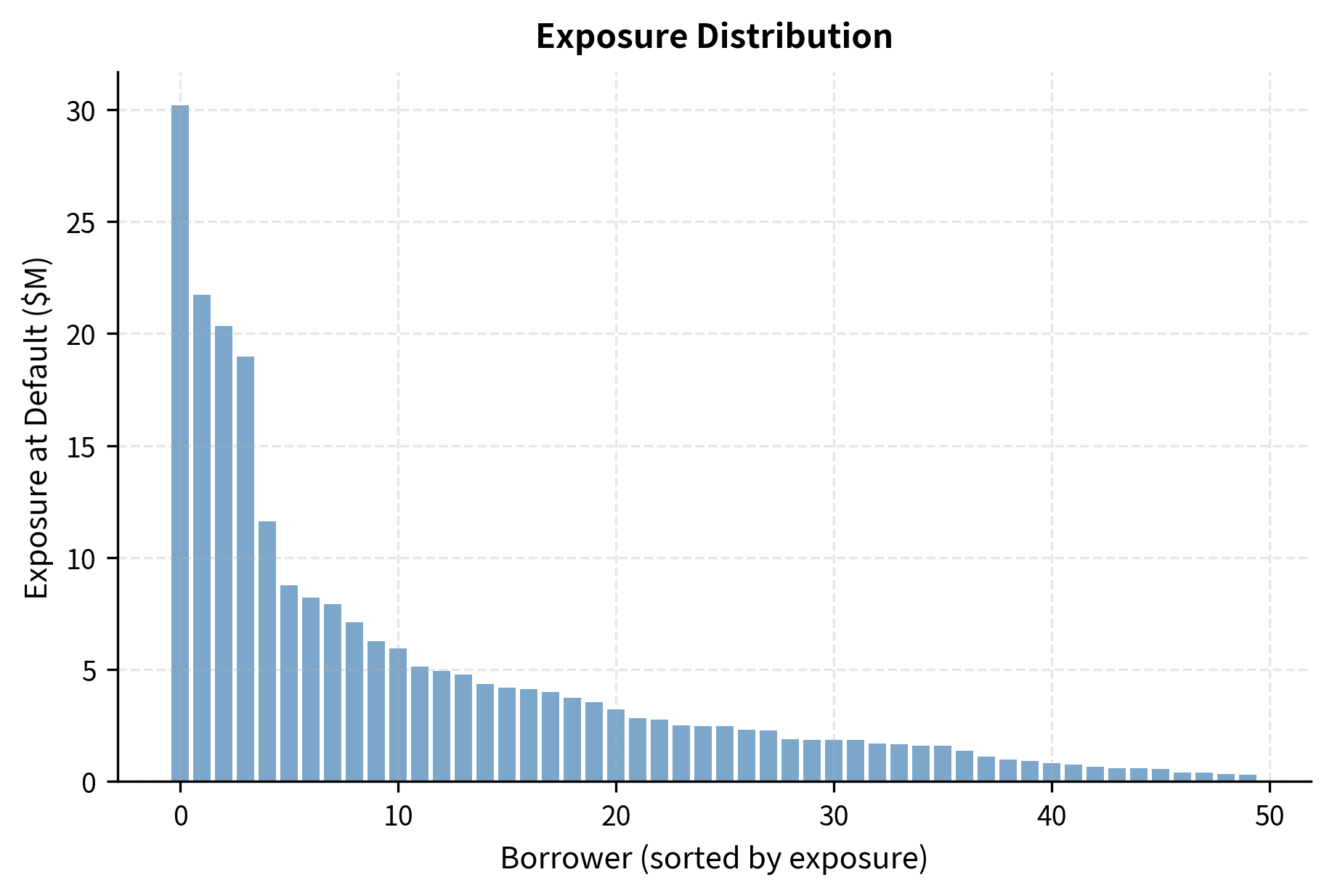
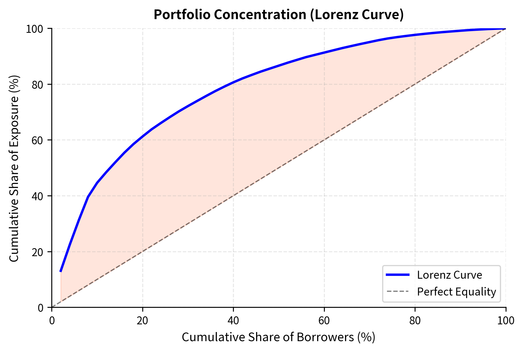
Individual loan metrics tell only part of the story. Portfolio effects, such as diversification and concentration, significantly affect total credit risk. A well-diversified portfolio of many small exposures to borrowers in different industries and regions will have much lower risk than a concentrated portfolio with large exposures to a few correlated borrowers. Understanding these portfolio dynamics is essential for managing credit risk at the enterprise level.

Default correlation substantially increases portfolio unexpected loss, and the magnitude of this effect is often surprising. During systemic crises, many borrowers deteriorate simultaneously, causing correlated defaults that overwhelm diversification benefits. When correlations spike, the portfolio that appeared well-diversified under normal conditions can experience concentrated losses. This phenomenon was tragically demonstrated in the structured credit market during 2008, when assumed correlations proved far too low. CDO tranches rated AAA based on historical correlation assumptions suffered unexpected losses because the underlying mortgage borrowers defaulted together at rates that the models had deemed virtually impossible.

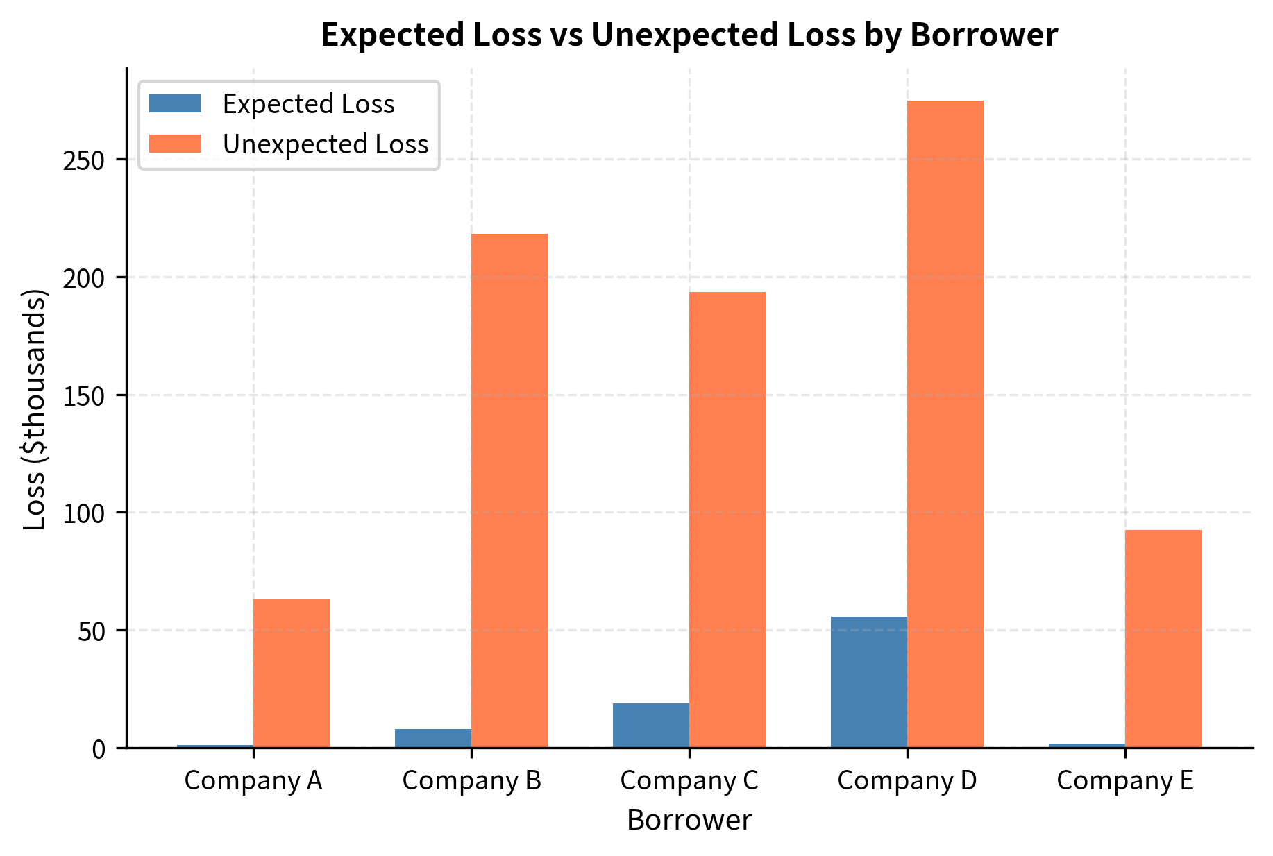
The comparison highlights the distinct drivers of credit risk components. Company D, with its high probability of default, contributes most to Expected Loss (blue bar). However, Company B generates the highest Unexpected Loss (coral bar) despite a better rating, driven by its large exposure size ($10M). This distinction is crucial for capital allocation, which focuses on buffering against unexpected rather than expected losses. Expected losses are a cost of doing business that should be covered by loan pricing and provisions; unexpected losses are the tail risks that require capital buffers to ensure institutional solvency.

Let's build a more complete credit risk analysis tool that incorporates the concepts we've covered. This implementation brings together PD, LGD, and EAD estimation with portfolio-level risk aggregation, demonstrating how the theoretical framework translates into practical applications:

The summary report provides a snapshot of the portfolio's risk profile. While the Expected Loss represents the average cost of credit (approximately 23 basis points), the Unexpected Loss and Credit VaR figures reveal the potential tail risk. The 99% Credit VaR indicates that in a 1-in-100 year adverse scenario, losses could exceed the expected level by a significant margin, driven by the correlation between borrowers. This VaR figure informs capital requirements: you need sufficient capital to absorb losses up to this level while remaining solvent.

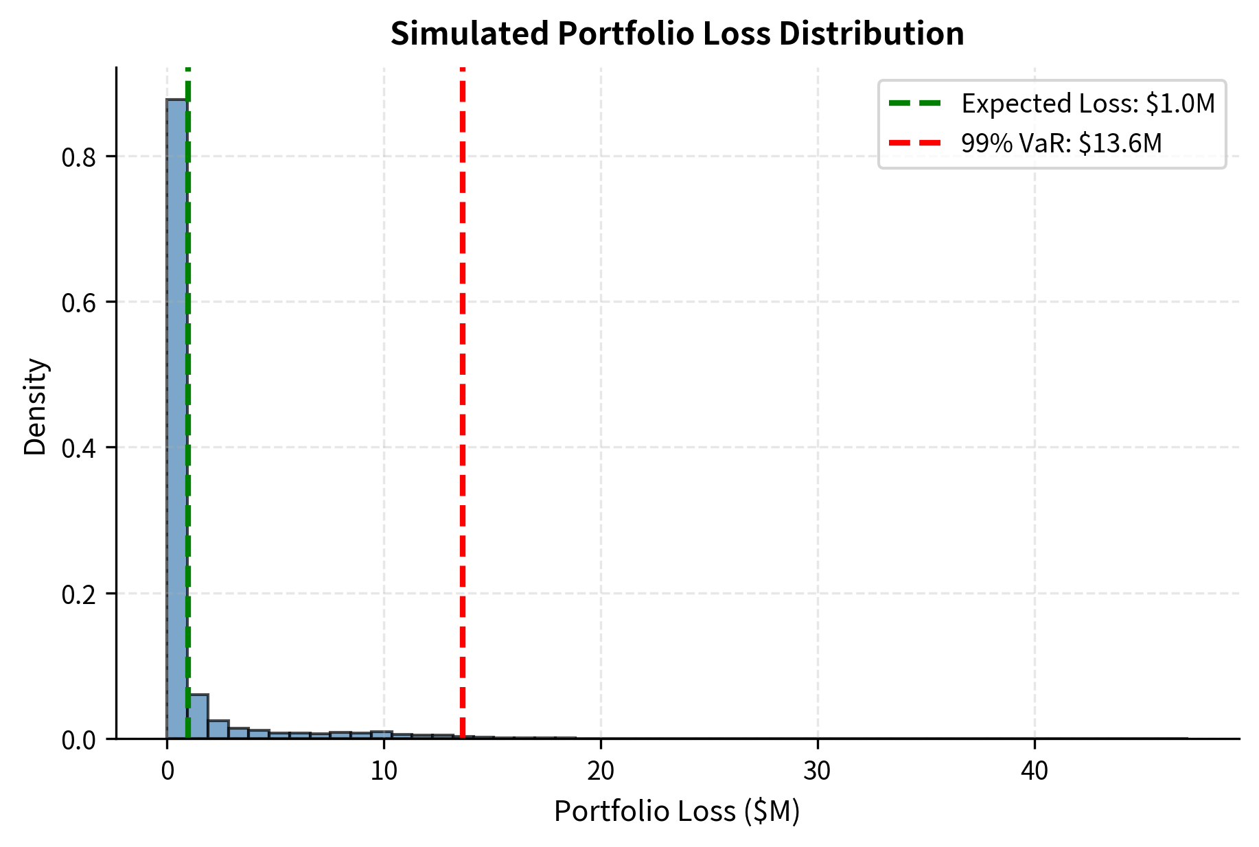
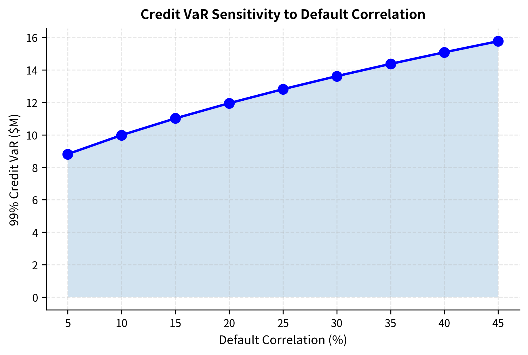
The simulation results demonstrate the heavy-tailed nature of credit losses. While expected loss provides a central estimate, the 99th percentile loss can be many times higher, especially when default correlation is significant. The sensitivity analysis in the second panel reveals just how dramatically Credit VaR increases with correlation: doubling the correlation assumption from 10% to 20% increases VaR by roughly 50%, and further increases to higher correlation levels continue this steep rise. This sensitivity underscores why correlation estimation is so critical and why model risk around correlation assumptions should be carefully monitored.

The key parameters for portfolio credit risk modeling are:

• PD (Probability of Default): Likelihood of borrower default, driving expected loss.
• LGD (Loss Given Default): Severity of loss, scaling the exposure at risk.
• EAD (Exposure at Default): Magnitude of the credit exposure.
• Default Correlation ($\rho$): The degree to which default events cluster. Higher correlation significantly increases tail risk (Unexpected Loss and VaR) while having no effect on Expected Loss.
• Confidence Level: The probability threshold for Value-at-Risk calculations (e.g., 99% or 99.9%).

The PD-LGD-EAD framework, while foundational, has important limitations that you must understand. No model perfectly captures reality, and awareness of these limitations is essential for sound risk management.

Parameter estimation uncertainty affects all components. PD estimates rely on historical data that may not reflect future conditions, particularly for low-default portfolios where statistical significance is limited. If only 1 in 500 investment-grade borrowers defaults annually, it takes many years to accumulate enough default observations for reliable estimation. LGD exhibits high variability and depends on factors that are difficult to observe in advance, such as the economic environment at the time of default and the specific circumstances of each bankruptcy. EAD for commitments and derivatives involves behavioral assumptions that may not hold under stress, as borrowers may act differently in crisis conditions than in normal times.

Correlation estimation is perhaps the weakest link in portfolio credit models. Default correlations are difficult to estimate empirically because defaults are rare events. We simply do not observe enough joint defaults under varying conditions to estimate correlations with precision. The correlations that matter most, those during systemic crises, are precisely the ones for which we have the least data, since such crises occur infrequently. The Basel framework addresses this by prescribing conservative correlation assumptions, but model risk remains substantial.

Point-in-time versus through-the-cycle tension creates practical challenges. Accounting standards (IFRS 9, CECL) require forward-looking expected credit loss provisions based on current conditions, while long-term business decisions benefit from cycle-average estimates. Institutions must maintain multiple PD frameworks for different purposes, reconciling potentially conflicting signals from each approach.

Model validation is constrained by the rarity of default events. Unlike market risk models that can be backtested against daily P&L, credit models produce predictions over long horizons with limited observable outcomes. This makes it difficult to distinguish between model accuracy and good fortune. A model that has performed well for ten years may simply have been lucky not to encounter conditions that reveal its flaws.

Despite these limitations, the EL = PD × LGD × EAD framework provides a disciplined structure for credit risk assessment. It forces explicit consideration of the key drivers of credit losses and enables consistent comparison across exposures. The next chapter extends this foundation to more sophisticated modeling approaches, including structural models and reduced-form credit risk models.

This chapter established the fundamental framework for measuring credit risk through its three core components:

Probability of Default (PD) measures the likelihood of borrower default over a specified horizon. PD can be estimated through credit ratings (providing stable, through-the-cycle assessments), market-implied approaches (extracting risk-neutral probabilities from CDS spreads), or structural models (treating equity as a call option on firm assets). The choice between through-the-cycle and point-in-time PD depends on the application.

Loss Given Default (LGD) captures the severity of loss when default occurs, typically expressed as 1 minus the recovery rate. LGD varies significantly by seniority, collateral, industry, and economic conditions. Crucially, recoveries tend to be lower precisely when default rates are high, creating procyclical credit losses.

Exposure at Default (EAD) quantifies the amount at risk when default occurs. For drawn loans, EAD is straightforward. For commitments and derivatives, EAD must account for potential drawdowns and exposure changes before default.

The expected loss formula, EL = PD × LGD × EAD, provides the foundation for loan pricing, provisioning, and portfolio risk assessment. However, unexpected loss and Credit VaR, which account for volatility around expected outcomes and default correlation, are equally important for capital allocation and risk limits.

Understanding these fundamentals prepares you for the more sophisticated credit risk modeling approaches we'll examine next, including the Merton structural model, CreditMetrics, and reduced-form intensity models.

Ready to test your understanding? Take this quick quiz to reinforce what you've learned about credit risk fundamentals.