Risk Management Practices: Limits, Hedging & Governance

Michael Brenndoerfer

Learn how to translate risk analytics into actionable controls through risk limits, hedging strategies, organizational governance, and regulatory frameworks.

Reading Level

Choose your expertise level to adjust how many terms are explained. Beginners see more tooltips, experts see fewer to maintain reading flow. Hover over underlined terms for instant definitions.

Risk Management Practices and PoliciesLink Copied

Measuring risk is only half the battle. The preceding chapters equipped you with sophisticated tools for quantifying market risk, credit risk, counterparty exposures, and liquidity risk. Yet a firm can possess the most advanced risk models in the industry and still suffer catastrophic losses if those measurements don't translate into disciplined action. Risk management practices and policies form the bridge between measurement and protection; they determine how risk information flows through an organization, who has authority to take risks, and what happens when limits are breached.

This chapter examines the operational infrastructure that transforms risk analytics into risk control. We'll explore how trading firms establish and enforce risk limits, how hedging strategies translate theoretical concepts into practical risk reduction, and how organizational structures from the Chief Risk Officer to risk committees ensure accountability. We'll also see how regulatory requirements shape risk management practices and why even unregulated hedge funds voluntarily adopt rigorous standards. Throughout, we'll emphasize that effective risk management is not a one-time exercise but a continuous feedback loop embedded in firm culture.

Risk Limits and Enforcement MechanismsLink Copied

Risk limits are the guardrails that keep a firm's risk-taking within acceptable bounds. They translate abstract risk appetite into concrete constraints that traders and portfolio managers must respect. Without well-designed limits and robust enforcement, risk measurement becomes an academic exercise: interesting but ineffective at preventing losses.

Types of Risk LimitsLink Copied

Financial institutions deploy multiple types of limits that work together to control risk from different angles. Each type addresses a specific aspect of risk exposure, and the combination provides defense in depth.

Value-at-Risk (VaR) limits constrain the maximum acceptable loss over a specified horizon at a given confidence level. As we discussed in the chapter on Market Risk Measurement, a $10 million daily Value-at-Risk (VaR) limit at 99% confidence means you expect losses to exceed $10 million on no more than 2-3 trading days per year. VaR limits are typically set at multiple levels:

Firm-wide VaR limit: The aggregate risk the entire organization can take
Desk-level VaR limits: Risk budgets allocated to individual trading desks
Trader-level VaR limits: Personal risk budgets for individual traders

The sum of desk-level limits typically exceeds the firm-wide limit because of diversification benefits; different desks often have partially offsetting positions.

Stop-loss limits trigger mandatory risk reduction after cumulative losses reach a threshold. Unlike VaR, which is forward-looking, stop-loss limits respond to realized losses. Common structures include:

Daily stop-loss: Requires a trader to close positions after losing a specified amount in a single day
Monthly stop-loss: Mandates risk reduction after cumulative monthly losses exceed a threshold
Trailing stop-loss: Triggers when losses from a recent high-water mark exceed a limit

Stop-loss limits serve a behavioral purpose as well as a financial one; they prevent traders from "doubling down" after losses in hopes of recovering.

Concentration limits prevent excessive exposure to any single source of risk. These take many forms:

Single-name limits: Maximum exposure to any individual issuer or counterparty
Sector limits: Maximum allocation to any industry sector
Geographic limits: Maximum exposure to any country or region
Asset class limits: Maximum allocation to equities, fixed income, or other asset classes
Tenor limits: Maximum exposure to any single maturity bucket

Greek limits constrain option portfolio sensitivities. Building on the Greeks from Part III, a derivatives trading desk might face:

Delta limits: Maximum directional exposure to underlying price movements
Gamma limits: Maximum exposure to acceleration in delta
Vega limits: Maximum exposure to implied volatility changes
Theta limits: Maximum time decay exposure

Stress test limits constrain potential losses under extreme but plausible scenarios. Rather than limiting statistical measures like VaR, these limits focus on what could happen in specific adverse events.

Limit Enforcement MechanismsLink Copied

Setting limits is straightforward; enforcing them is where risk management proves its worth. Enforcement requires infrastructure, clear escalation procedures, and consequences for violations.

Real-Time Monitoring Systems track risk metrics continuously and alert relevant personnel when positions approach or breach limits. Modern trading operations maintain dashboards that display:

Current utilization of each limit as a percentage of the maximum
Trend of utilization over recent periods
Projected utilization based on pending trades
Color-coded warnings (green, yellow, red) as limits approach

Pre-Trade Compliance Checks intercept trades before execution to verify they won't cause limit breaches. Order management systems calculate the pro forma impact of proposed trades and block those that would violate limits unless override authorization is obtained.

Hard Limits vs. Soft Limits represent different enforcement philosophies. Hard limits cannot be breached under any circumstances; the trading system simply refuses to execute violating trades. Soft limits can be breached temporarily with appropriate authorization, acknowledging that rigid constraints sometimes interfere with legitimate trading needs.

Escalation Procedures define what happens when limits are approached or breached:

Warning threshold (e.g., 80% utilization): Automated alert to trader and supervisor
Soft breach threshold (e.g., 100% utilization): Requires supervisor approval to continue
Hard breach threshold (e.g., 110% utilization): Mandatory position reduction within specified timeframe
Severe breach (e.g., 125% utilization): Immediate trading suspension and executive escalation

Consequences for Violations range from warnings to termination depending on severity and pattern. Even when violations result from market movements rather than trader actions, repeated occurrences may indicate poor position management.

In[2]:

Code

import pandas as pd
from dataclasses import dataclass
from typing import Dict, List
from datetime import datetime


@dataclass
class RiskLimit:
    """Represents a risk limit with warning and breach thresholds."""

    name: str
    limit_value: float
    warning_threshold: float = 0.80  # Warning at 80% utilization
    soft_breach_threshold: float = 1.00  # Soft breach at 100%
    hard_breach_threshold: float = 1.10  # Hard breach at 110%

    def check_utilization(self, current_value: float) -> str:
        """Check limit utilization and return status."""
        utilization = abs(current_value) / self.limit_value

        if utilization >= self.hard_breach_threshold:
            return "HARD_BREACH"
        elif utilization >= self.soft_breach_threshold:
            return "SOFT_BREACH"
        elif utilization >= self.warning_threshold:
            return "WARNING"
        else:
            return "OK"

    def utilization_pct(self, current_value: float) -> float:
        """Return utilization as percentage."""
        return abs(current_value) / self.limit_value * 100


class TradingDeskRiskMonitor:
    """Monitor risk limits for a trading desk."""

    def __init__(self, desk_name: str):
        self.desk_name = desk_name
        self.limits: Dict[str, RiskLimit] = {}
        self.current_values: Dict[str, float] = {}
        self.breach_history: List[Dict] = []

    def add_limit(self, limit: RiskLimit):
        """Add a risk limit to monitor."""
        self.limits[limit.name] = limit
        self.current_values[limit.name] = 0.0

    def update_exposure(self, limit_name: str, value: float):
        """Update current exposure for a limit."""
        if limit_name not in self.limits:
            raise ValueError(f"Unknown limit: {limit_name}")

        self.current_values[limit_name] = value
        status = self.limits[limit_name].check_utilization(value)

        if status in ["SOFT_BREACH", "HARD_BREACH"]:
            self.breach_history.append(
                {
                    "timestamp": datetime.now(),
                    "limit_name": limit_name,
                    "value": value,
                    "status": status,
                }
            )

        return status

    def get_dashboard(self) -> pd.DataFrame:
        """Generate risk dashboard showing all limits."""
        data = []
        for name, limit in self.limits.items():
            current = self.current_values[name]
            data.append(
                {
                    "Limit Name": name,
                    "Current Value": current,
                    "Limit": limit.limit_value,
                    "Utilization %": limit.utilization_pct(current),
                    "Status": limit.check_utilization(current),
                }
            )
        return pd.DataFrame(data)

import pandas as pd
from dataclasses import dataclass
from typing import Dict, List
from datetime import datetime


@dataclass
class RiskLimit:
    """Represents a risk limit with warning and breach thresholds."""

    name: str
    limit_value: float
    warning_threshold: float = 0.80  # Warning at 80% utilization
    soft_breach_threshold: float = 1.00  # Soft breach at 100%
    hard_breach_threshold: float = 1.10  # Hard breach at 110%

    def check_utilization(self, current_value: float) -> str:
        """Check limit utilization and return status."""
        utilization = abs(current_value) / self.limit_value

        if utilization >= self.hard_breach_threshold:
            return "HARD_BREACH"
        elif utilization >= self.soft_breach_threshold:
            return "SOFT_BREACH"
        elif utilization >= self.warning_threshold:
            return "WARNING"
        else:
            return "OK"

    def utilization_pct(self, current_value: float) -> float:
        """Return utilization as percentage."""
        return abs(current_value) / self.limit_value * 100


class TradingDeskRiskMonitor:
    """Monitor risk limits for a trading desk."""

    def __init__(self, desk_name: str):
        self.desk_name = desk_name
        self.limits: Dict[str, RiskLimit] = {}
        self.current_values: Dict[str, float] = {}
        self.breach_history: List[Dict] = []

    def add_limit(self, limit: RiskLimit):
        """Add a risk limit to monitor."""
        self.limits[limit.name] = limit
        self.current_values[limit.name] = 0.0

    def update_exposure(self, limit_name: str, value: float):
        """Update current exposure for a limit."""
        if limit_name not in self.limits:
            raise ValueError(f"Unknown limit: {limit_name}")

        self.current_values[limit_name] = value
        status = self.limits[limit_name].check_utilization(value)

        if status in ["SOFT_BREACH", "HARD_BREACH"]:
            self.breach_history.append(
                {
                    "timestamp": datetime.now(),
                    "limit_name": limit_name,
                    "value": value,
                    "status": status,
                }
            )

        return status

    def get_dashboard(self) -> pd.DataFrame:
        """Generate risk dashboard showing all limits."""
        data = []
        for name, limit in self.limits.items():
            current = self.current_values[name]
            data.append(
                {
                    "Limit Name": name,
                    "Current Value": current,
                    "Limit": limit.limit_value,
                    "Utilization %": limit.utilization_pct(current),
                    "Status": limit.check_utilization(current),
                }
            )
        return pd.DataFrame(data)

In[3]:

Code

import numpy as np

# Create a trading desk risk monitor
equity_desk = TradingDeskRiskMonitor("Equity Trading")

# Add various risk limits
equity_desk.add_limit(RiskLimit("Daily VaR", limit_value=5_000_000))
equity_desk.add_limit(RiskLimit("Single Name Exposure", limit_value=10_000_000))
equity_desk.add_limit(RiskLimit("Sector Concentration", limit_value=25_000_000))
equity_desk.add_limit(RiskLimit("Delta Exposure", limit_value=50_000_000))
equity_desk.add_limit(RiskLimit("Daily Stop Loss", limit_value=2_000_000))

# Simulate current exposures
np.random.seed(42)
equity_desk.update_exposure("Daily VaR", 3_800_000)  # 76% - OK
equity_desk.update_exposure("Single Name Exposure", 8_500_000)  # 85% - Warning
equity_desk.update_exposure(
    "Sector Concentration", 26_000_000
)  # 104% - Soft breach
equity_desk.update_exposure("Delta Exposure", 35_000_000)  # 70% - OK
equity_desk.update_exposure("Daily Stop Loss", 1_200_000)  # 60% - OK

import numpy as np

# Create a trading desk risk monitor
equity_desk = TradingDeskRiskMonitor("Equity Trading")

# Add various risk limits
equity_desk.add_limit(RiskLimit("Daily VaR", limit_value=5_000_000))
equity_desk.add_limit(RiskLimit("Single Name Exposure", limit_value=10_000_000))
equity_desk.add_limit(RiskLimit("Sector Concentration", limit_value=25_000_000))
equity_desk.add_limit(RiskLimit("Delta Exposure", limit_value=50_000_000))
equity_desk.add_limit(RiskLimit("Daily Stop Loss", limit_value=2_000_000))

# Simulate current exposures
np.random.seed(42)
equity_desk.update_exposure("Daily VaR", 3_800_000)  # 76% - OK
equity_desk.update_exposure("Single Name Exposure", 8_500_000)  # 85% - Warning
equity_desk.update_exposure(
    "Sector Concentration", 26_000_000
)  # 104% - Soft breach
equity_desk.update_exposure("Delta Exposure", 35_000_000)  # 70% - OK
equity_desk.update_exposure("Daily Stop Loss", 1_200_000)  # 60% - OK

Out[4]:

Console

Risk Dashboard: Equity Trading
================================================================================
          Limit Name Current Value       Limit Utilization %        Status
           Daily VaR    $3,800,000  $5,000,000         76.0%          🟢 OK
Single Name Exposure    $8,500,000 $10,000,000         85.0%     🟡 WARNING
Sector Concentration   $26,000,000 $25,000,000        104.0% 🟠 SOFT_BREACH
      Delta Exposure   $35,000,000 $50,000,000         70.0%          🟢 OK
     Daily Stop Loss    $1,200,000  $2,000,000         60.0%          🟢 OK

Out[5]:

Visualization

Risk limit utilization dashboard showing current exposure as a percentage of each limit. Horizontal lines indicate warning (80%), soft breach (100%), and hard breach (110%) thresholds. The Sector Concentration limit is in breach, requiring immediate attention.

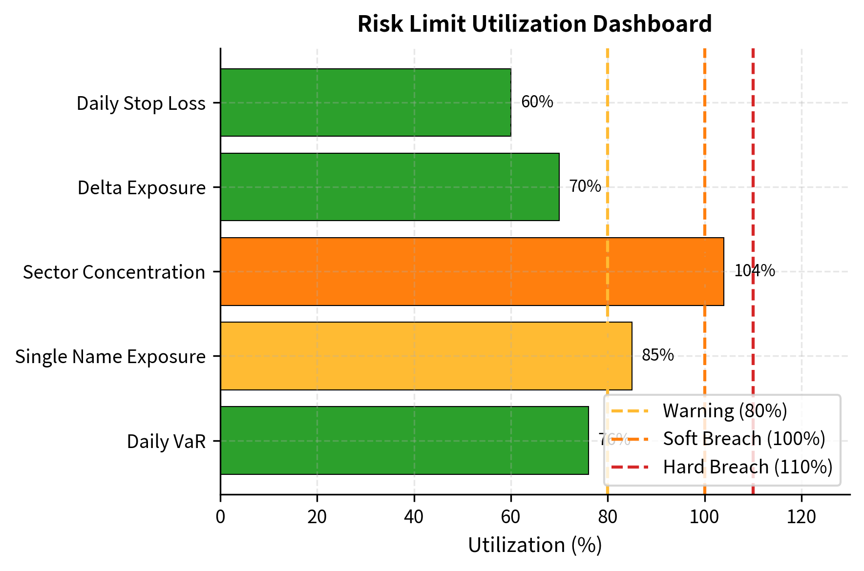
The dashboard reveals that the Sector Concentration limit has been breached (104% utilization), requiring immediate attention. The Single Name Exposure is in warning territory at 85% utilization, suggesting the desk should be cautious about adding to that position.

Dynamic Limit AdjustmentLink Copied

Risk limits are not static; they should evolve with market conditions, firm strategy, and lessons learned. Several factors drive limit adjustments:

Volatility regimes may trigger automatic limit scaling. During periods of elevated market volatility, a firm might temporarily reduce VaR limits to maintain the same expected frequency of limit breaches. If market VaR doubles due to increased volatility, maintaining the same dollar limit effectively allows twice the expected loss frequency.

Performance can influence limits through dynamic allocation. Desks with strong risk-adjusted returns may receive increased risk budgets, while consistently underperforming desks may see reductions.

Seasonal patterns in liquidity may warrant limit adjustments. Year-end periods often see reduced market liquidity, justifying tighter limits. Similarly, limits might be reduced ahead of known high-volatility events like central bank announcements or elections.

Correlation changes affect the diversification assumptions underlying aggregate limits. If correlations increase during market stress (as they typically do), the diversification benefit assumed when allocating desk limits decreases, potentially requiring aggregate limit reductions.

Hedging Strategies in PracticeLink Copied

Hedging transforms risk management from passive measurement to active intervention. While we covered derivatives and their theoretical applications in Part II and option Greeks in Part III, translating these concepts into practical hedging programs requires additional considerations around cost, basis risk, and operational complexity.

Hedging Objectives and TradeoffsLink Copied

Before implementing a hedge, you must clarify what outcome you seek. Different objectives lead to different hedging strategies:

Variance minimization seeks the smallest possible volatility of the hedged position. This approach, grounded in the mean-variance framework from Part IV, minimizes the variance of portfolio returns regardless of expected return impact.
Downside protection focuses specifically on adverse outcomes while preserving upside participation. Options-based strategies naturally provide this asymmetric protection, though at the cost of the option premium.
Cash flow stabilization aims to reduce variability in future cash flows rather than mark-to-market values. Corporations hedging future revenues or expenses often prioritize this objective.
Regulatory capital reduction hedges to reduce risk-weighted assets and associated capital requirements, even if the hedge doesn't meaningfully reduce economic risk.

These objectives often conflict. The minimum-variance hedge might lock in unfavorable prices, while downside protection requires paying premiums that reduce expected returns. We must balance these tradeoffs against firm priorities.

Linear Hedging with Forwards and FuturesLink Copied

Forwards and futures provide symmetric hedging, meaning they reduce both upside and downside exposure proportionally. When a firm uses a futures contract to hedge an existing position, any gain on one side is offset by a corresponding loss on the other. This symmetric payoff structure makes linear instruments the foundation of most corporate and institutional hedging programs. Building on the pricing relationships from Part II, let's examine how we determine the optimal hedge and implement it effectively.

The central question in any hedging program is: how much of the hedge instrument should we trade relative to our underlying exposure? A naive approach might suggest a one-to-one ratio, but this ignores important statistical relationships between the asset being hedged and the instrument used for hedging. When these instruments move differently, whether due to basis risk, differing volatilities, or imperfect correlation, a more sophisticated approach is required.

The hedge ratio determines how many contracts to trade relative to the underlying exposure. The goal of minimum-variance hedging is to find the ratio that minimizes the total volatility of the combined position, consisting of the original exposure plus the hedge. This optimization problem has a closed-form solution derived from basic portfolio theory.

To understand the intuition, consider that we want to minimize the variance of the hedged portfolio's returns. If we denote the spot position's return as $R_S$ and the futures return as $R_F$ , then the hedged portfolio return is $R_S - h \cdot R_F$ , where $h$ is the hedge ratio. Taking the derivative of the variance of this expression with respect to $h$ and setting it equal to zero yields the optimal hedge ratio:

h^* = \rho \frac{\sigma_S}{\sigma_F}

where:

$h^*$ : optimal hedge ratio (units of futures per unit of spot)
$\rho$ : correlation coefficient between spot and futures returns
$\sigma_S$ : volatility (standard deviation) of spot returns
$\sigma_F$ : volatility (standard deviation) of futures returns

This elegant formula captures two fundamental adjustments that you must make. First, the ratio of volatilities $\sigma_S/\sigma_F$ accounts for the relative riskiness of the spot position versus the hedge instrument. If the futures contract is less volatile than the underlying asset, a larger futures position is needed to offset each unit of spot risk. Conversely, if futures are more volatile, a smaller position suffices. Think of this as matching the "risk magnitude" between what you hold and what you use to hedge.

Second, the correlation term $\rho$ reflects the degree to which the two instruments move together. Perfect correlation ( $\rho = 1$ ) means every movement in the spot price is mirrored by a proportional movement in the futures price, so the full volatility-adjusted hedge is appropriate. However, when correlation is less than perfect, some portion of the hedge position introduces noise rather than risk reduction. The hedge ratio is scaled down by $\rho$ to avoid adding uncompensated variance, recognizing that an imperfect hedge instrument can actually increase portfolio variance if used too aggressively.

Consider a practical example: a jet fuel consumer wants to hedge fuel price risk using crude oil futures. Jet fuel and crude oil prices are closely related, both driven by global energy supply and demand, but they don't move in lockstep. Refining margins fluctuate, regional supply disruptions affect jet fuel differently than crude, and specification differences create additional basis risk. The minimum-variance hedge ratio quantifies exactly how these statistical relationships should inform the hedge size.

In[6]:

Code

def calculate_optimal_hedge_ratio(
    spot_returns: np.ndarray, futures_returns: np.ndarray
) -> dict:
    """
    Calculate the minimum variance hedge ratio.

    Parameters
    ----------
    spot_returns : np.ndarray
        Historical returns of the spot position
    futures_returns : np.ndarray
        Historical returns of the futures contract

    Returns
    -------
    dict
        Hedge ratio and hedging effectiveness statistics
    """
    # Calculate statistics
    spot_vol = np.std(spot_returns)
    futures_vol = np.std(futures_returns)
    correlation = np.corrcoef(spot_returns, futures_returns)[0, 1]

    # Minimum variance hedge ratio
    hedge_ratio = correlation * (spot_vol / futures_vol)

    # Calculate hedging effectiveness (R-squared of the hedge)
    # This is the proportion of variance eliminated by hedging
    hedging_effectiveness = correlation**2

    # Calculate residual volatility after hedging
    hedged_returns = spot_returns - hedge_ratio * futures_returns
    residual_vol = np.std(hedged_returns)
    variance_reduction = 1 - (residual_vol**2) / (spot_vol**2)

    return {
        "hedge_ratio": hedge_ratio,
        "correlation": correlation,
        "spot_volatility": spot_vol,
        "futures_volatility": futures_vol,
        "hedging_effectiveness": hedging_effectiveness,
        "residual_volatility": residual_vol,
        "variance_reduction": variance_reduction,
    }

def calculate_optimal_hedge_ratio(
    spot_returns: np.ndarray, futures_returns: np.ndarray
) -> dict:
    """
    Calculate the minimum variance hedge ratio.

    Parameters
    ----------
    spot_returns : np.ndarray
        Historical returns of the spot position
    futures_returns : np.ndarray
        Historical returns of the futures contract

    Returns
    -------
    dict
        Hedge ratio and hedging effectiveness statistics
    """
    # Calculate statistics
    spot_vol = np.std(spot_returns)
    futures_vol = np.std(futures_returns)
    correlation = np.corrcoef(spot_returns, futures_returns)[0, 1]

    # Minimum variance hedge ratio
    hedge_ratio = correlation * (spot_vol / futures_vol)

    # Calculate hedging effectiveness (R-squared of the hedge)
    # This is the proportion of variance eliminated by hedging
    hedging_effectiveness = correlation**2

    # Calculate residual volatility after hedging
    hedged_returns = spot_returns - hedge_ratio * futures_returns
    residual_vol = np.std(hedged_returns)
    variance_reduction = 1 - (residual_vol**2) / (spot_vol**2)

    return {
        "hedge_ratio": hedge_ratio,
        "correlation": correlation,
        "spot_volatility": spot_vol,
        "futures_volatility": futures_vol,
        "hedging_effectiveness": hedging_effectiveness,
        "residual_volatility": residual_vol,
        "variance_reduction": variance_reduction,
    }

In[7]:

Code

# Simulate a hedging scenario: corporate hedging jet fuel with crude oil futures
np.random.seed(42)
n_days = 252

# Common factor driving both prices
common_factor = np.random.normal(0, 0.02, n_days)

# Crude oil futures returns (hedge instrument) - correlated but not perfectly
crude_returns = 0.85 * common_factor + np.random.normal(0, 0.012, n_days)

# Jet fuel spot returns (what the company is exposed to)
jet_fuel_returns = 0.85 * common_factor + np.random.normal(0, 0.014, n_days)

hedge_analysis = calculate_optimal_hedge_ratio(jet_fuel_returns, crude_returns)

# Simulate a hedging scenario: corporate hedging jet fuel with crude oil futures
np.random.seed(42)
n_days = 252

# Common factor driving both prices
common_factor = np.random.normal(0, 0.02, n_days)

# Crude oil futures returns (hedge instrument) - correlated but not perfectly
crude_returns = 0.85 * common_factor + np.random.normal(0, 0.012, n_days)

# Jet fuel spot returns (what the company is exposed to)
jet_fuel_returns = 0.85 * common_factor + np.random.normal(0, 0.014, n_days)

hedge_analysis = calculate_optimal_hedge_ratio(jet_fuel_returns, crude_returns)

Out[8]:

Console

Jet Fuel Hedging Analysis with Crude Oil Futures
==================================================
Optimal hedge ratio: 0.659
Correlation: 0.602
Spot volatility (annualized): 35.7%
Futures volatility (annualized): 32.6%
Hedging effectiveness (R²): 36.3%
Variance reduction achieved: 36.3%
Residual volatility (annualized): 28.5%

Out[9]:

Visualization

Portfolio variance as a function of hedge ratio. The minimum variance occurs at the optimal hedge ratio (dashed line), where the tradeoff between hedging benefit and basis risk is balanced. Deviating from the optimal ratio in either direction increases portfolio variance.

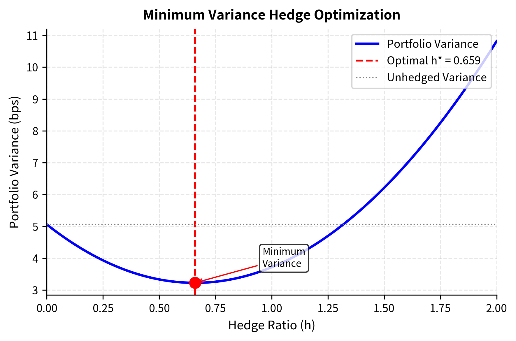
The analysis shows that despite a high correlation, imperfect correlation between jet fuel and crude oil creates basis risk: the risk that the hedge instrument and the underlying exposure don't move in perfect lockstep. The hedging effectiveness of approximately 72% means about 28% of the original variance remains after hedging. This residual risk is irreducible given the available hedge instrument; it represents the price paid for not having access to a jet fuel futures contract that perfectly matches the exposure. Understanding this limitation is crucial because it reminds you that hedging reduces but rarely eliminates risk entirely.

Out[10]:

Visualization

Relationship between correlation and hedging effectiveness (R-squared). Hedging effectiveness equals the square of the correlation coefficient, meaning a correlation of 0.85 yields only 72% variance reduction. This demonstrates why cross-hedging with imperfect instruments always leaves residual basis risk.

Key ParametersLink Copied

The key parameters for the Minimum Variance Hedge Ratio deserve careful attention because understanding them illuminates the fundamental tradeoffs in any hedging decision:

$\rho$ : Correlation coefficient between spot and futures returns. This parameter ranges from -1 to +1 and measures how closely the hedge instrument tracks the underlying exposure. Higher correlation improves hedging effectiveness because movements in the hedge more reliably offset movements in the spot position. When selecting among multiple possible hedge instruments, correlation is often the primary selection criterion. A correlation of 0.85 means the two assets share about 72% of their variance (since $0.85^2 \approx 0.72$ ), providing substantial but imperfect risk reduction.
$\sigma_S$ : Volatility of the spot position, meaning the underlying exposure being hedged. This captures the magnitude of risk in the original position. Higher spot volatility indicates greater potential for adverse price movements and typically motivates more urgent hedging activity. The spot volatility enters the numerator of the hedge ratio formula because more volatile exposures require proportionally larger hedges.
$\sigma_F$ : Volatility of the futures contract or hedge instrument. This measures how much the hedge instrument itself fluctuates. The futures volatility enters the denominator of the formula, reflecting the intuition that more volatile hedge instruments have greater "power" to offset risk, so fewer contracts are needed. If futures are twice as volatile as the spot, roughly half as many contracts provide the same risk offset.
$h^*$ : Optimal hedge ratio, representing the number of futures units needed per unit of spot exposure to minimize total portfolio variance. This ratio emerges from the mathematical optimization and may be greater than, less than, or equal to 1.0 depending on the relative volatilities and correlation. A ratio of 0.95 means for every 100 units of spot exposure, 95 units of futures provides the minimum-variance hedge.

Options-Based Hedging StrategiesLink Copied

Options provide asymmetric protection that futures cannot offer, representing a fundamentally different approach to managing risk. While futures lock in a price regardless of subsequent market movements, options allow you to participate in favorable outcomes while establishing a floor against adverse ones. This asymmetry comes at a cost, specifically the option premium, but it addresses a critical limitation of linear hedging: the sacrifice of potential gains.

The key strategies mirror those discussed in the Option Strategies chapter but are deployed here specifically for risk management rather than speculation. When you use options to hedge, the objective shifts from profiting from directional views to protecting existing value. This distinction matters because it affects strike selection, tenor choice, and the willingness to pay premium.

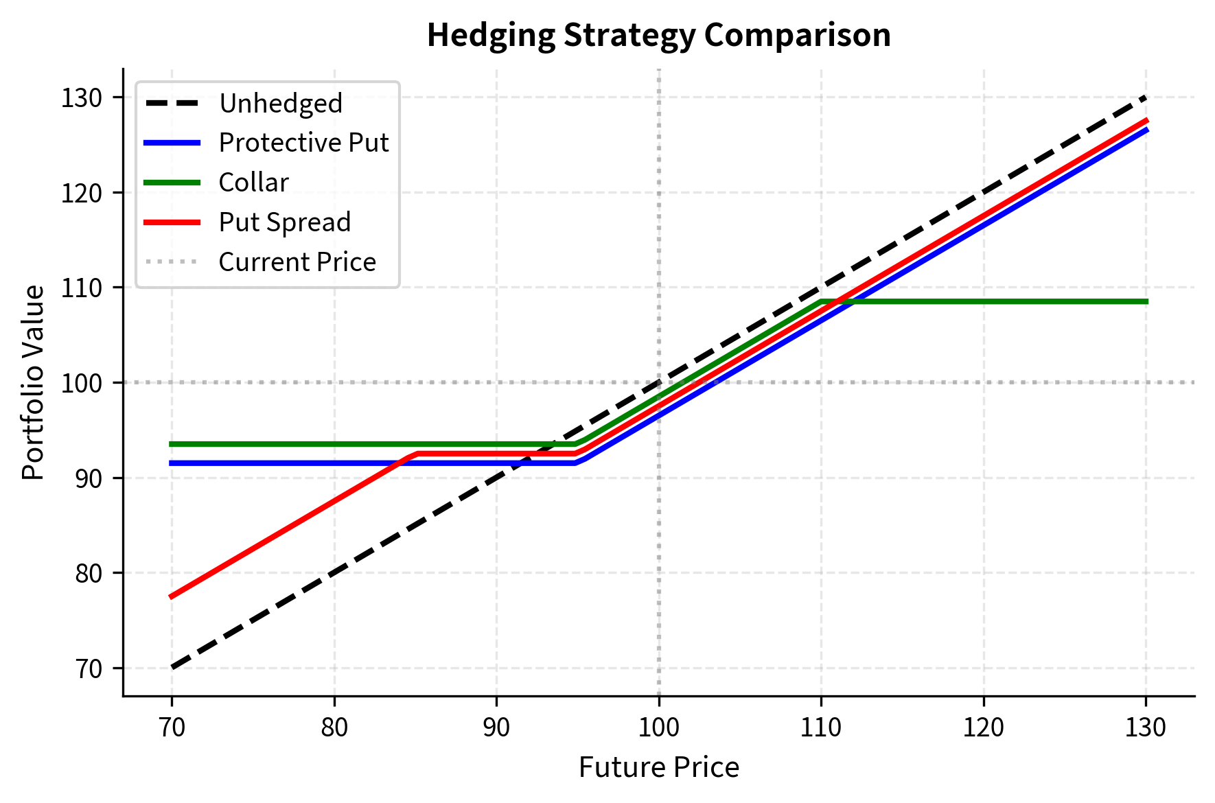
Protective puts establish a floor on portfolio value by granting the right to sell at the strike price regardless of how far the market falls. If you hold $100 million in equities, you might purchase at-the-money puts with a notional of $100 million. If the market declines 20%, the put gains value to offset most of the portfolio loss. If the market rises 20%, the put expires worthless, but the portfolio participates fully in the gain. The put premium is the cost of insurance, functioning economically just like paying for property or casualty insurance. The strike determines the floor, with lower strikes offering cheaper protection but a higher deductible.

Collars reduce hedging cost by sacrificing upside participation. The strategy involves simultaneously buying protective puts and selling out-of-the-money calls, with the call premium partially or fully financing the put purchase. When the call strike is chosen so that its premium exactly offsets the put premium, the collar is said to be "zero-cost," though this terminology is somewhat misleading since you give up potentially valuable upside. Collars appeal to you if you have specific return thresholds you need to protect and are willing to cap returns above a certain level in exchange for downside protection.

Put spreads further reduce cost by limiting the depth of protection. This strategy involves buying puts at one strike while selling puts at a lower strike, creating a protected zone between the two strikes but leaving the portfolio exposed to losses beyond the lower strike. The maximum loss on the hedged portfolio occurs at or below the lower strike, after which the short put position offsets further gains on the long put. Put spreads are appropriate when you are primarily concerned about moderate market declines rather than catastrophic scenarios, or when premium budgets are constrained.

In[11]:

Code

def analyze_hedging_strategies(
    current_price: float,
    put_strike: float,
    call_strike: float,
    put_premium: float,
    call_premium: float,
    lower_put_strike: float = None,
    lower_put_premium: float = None,
) -> pd.DataFrame:
    """
    Compare portfolio outcomes under different hedging strategies.
    """
    # Range of possible future prices
    prices = np.linspace(current_price * 0.7, current_price * 1.3, 100)

    results = pd.DataFrame({"Future Price": prices})

    # Unhedged portfolio value
    results["Unhedged"] = prices

    # Protective put
    put_payoff = np.maximum(put_strike - prices, 0)
    results["Protective Put"] = prices + put_payoff - put_premium

    # Collar (long put, short call)
    call_payoff = np.maximum(prices - call_strike, 0)
    collar_cost = put_premium - call_premium
    results["Collar"] = prices + put_payoff - call_payoff - collar_cost

    # Put spread (if lower strike provided)
    if lower_put_strike is not None and lower_put_premium is not None:
        lower_put_payoff = np.maximum(lower_put_strike - prices, 0)
        spread_cost = put_premium - lower_put_premium
        results["Put Spread"] = (
            prices + put_payoff - lower_put_payoff - spread_cost
        )

    return results

def analyze_hedging_strategies(
    current_price: float,
    put_strike: float,
    call_strike: float,
    put_premium: float,
    call_premium: float,
    lower_put_strike: float = None,
    lower_put_premium: float = None,
) -> pd.DataFrame:
    """
    Compare portfolio outcomes under different hedging strategies.
    """
    # Range of possible future prices
    prices = np.linspace(current_price * 0.7, current_price * 1.3, 100)

    results = pd.DataFrame({"Future Price": prices})

    # Unhedged portfolio value
    results["Unhedged"] = prices

    # Protective put
    put_payoff = np.maximum(put_strike - prices, 0)
    results["Protective Put"] = prices + put_payoff - put_premium

    # Collar (long put, short call)
    call_payoff = np.maximum(prices - call_strike, 0)
    collar_cost = put_premium - call_premium
    results["Collar"] = prices + put_payoff - call_payoff - collar_cost

    # Put spread (if lower strike provided)
    if lower_put_strike is not None and lower_put_premium is not None:
        lower_put_payoff = np.maximum(lower_put_strike - prices, 0)
        spread_cost = put_premium - lower_put_premium
        results["Put Spread"] = (
            prices + put_payoff - lower_put_payoff - spread_cost
        )

    return results

In[12]:

Code

# Portfolio hedging example
current_price = 100
put_strike = 95  # 5% OTM put for protection
call_strike = 110  # 10% OTM call for collar
put_premium = 3.5
call_premium = 2.0
lower_put_strike = 85  # For put spread
lower_put_premium = 1.0

hedge_comparison = analyze_hedging_strategies(
    current_price,
    put_strike,
    call_strike,
    put_premium,
    call_premium,
    lower_put_strike,
    lower_put_premium,
)

# Portfolio hedging example
current_price = 100
put_strike = 95  # 5% OTM put for protection
call_strike = 110  # 10% OTM call for collar
put_premium = 3.5
call_premium = 2.0
lower_put_strike = 85  # For put spread
lower_put_premium = 1.0

hedge_comparison = analyze_hedging_strategies(
    current_price,
    put_strike,
    call_strike,
    put_premium,
    call_premium,
    lower_put_strike,
    lower_put_premium,
)

Out[13]:

Visualization

Line chart comparing unhedged portfolio value against protective put, collar, and put spread hedging strategies across price scenarios. — Comparison of hedging strategies showing portfolio value at expiration under different future price scenarios. The protective put provides unlimited upside with a floor at the strike, while the collar caps both upside and downside. The put spread offers limited protection at lower cost.

The protective put provides a clear floor (at the strike minus the premium paid) while preserving full upside participation. The collar eliminates most of the insurance cost but caps upside at the call strike. The put spread offers cheaper protection but only for a limited range of downside moves.

Key ParametersLink Copied

The key parameters for Options Hedging Strategies reflect the fundamental tradeoffs between cost, protection depth, and upside participation that you must navigate:

Strike Price ( $K$ ): The price at which the option can be exercised, determining the level at which protection engages. For puts, the strike establishes the floor below which the hedge provides compensation for further losses. For calls in a collar, the strike sets the ceiling where upside gains are capped. Strike selection involves balancing the desire for more complete protection (higher put strikes) against the cost of that protection (higher premiums). Strikes are often quoted in terms of moneyness, such as "5% out-of-the-money," which relates the strike to the current underlying price.
Premium: The cost to purchase the option, representing the "insurance" cost for protective strategies. Premium depends on strike, time to expiration, volatility, and interest rates, as explored in Part III on option pricing. The premium is paid upfront and is lost whether or not the option is ultimately exercised, making it analogous to an insurance premium. When evaluating hedging cost, you often express premium as a percentage of the notional being protected, providing a standardized measure comparable across different position sizes.
Underlying Price ( $S$ ): The current price of the asset being hedged, which establishes the starting point for evaluating protection. The relationship between $S$ and $K$ determines the option's moneyness and thus its premium. At-the-money options (where $K \approx S$ ) cost more than out-of-the-money options but provide more immediate protection. The underlying price also determines the notional size of the hedge, since option contracts typically control a standardized number of underlying units.

Delta Hedging for Options PortfoliosLink Copied

Options market makers and proprietary trading desks typically hedge their directional exposure dynamically through delta hedging, which represents a fundamentally different hedging paradigm from the static approaches discussed above. Rather than establishing a fixed hedge at the outset and holding it through expiration, delta hedging involves continuously adjusting the hedge as market conditions change. This dynamic approach is essential for you if you maintain large portfolios of options and need to manage directional exposure on an ongoing basis.

As we discussed in the Greeks chapter, delta measures the sensitivity of option value to underlying price changes. A call option with a delta of 0.50 gains approximately \ $0.50 in value for each \\$ 1 increase in the underlying price. By holding an offsetting position in the underlying equal to the negative of delta, you neutralize the first-order price sensitivity. For example, shorting 50 shares against a long call with 0.50 delta creates a portfolio with approximately zero sensitivity to small price moves.

The key word is "approximately," because delta itself changes as the underlying price moves. This is where gamma, the second derivative of option value with respect to price, becomes critical. High-gamma positions see their deltas change rapidly, requiring frequent rebalancing to maintain delta neutrality. Conversely, low-gamma positions remain approximately neutral for longer periods, reducing the need for adjustment.

The practical challenges of delta hedging include several important considerations:

Transaction costs erode profits with every hedge adjustment. Each rebalancing trade incurs commissions, bid-ask spreads, and market impact costs. You must balance hedging precision against trading costs, often accepting some residual delta exposure to avoid the expense of continuous adjustment.

Discrete hedging introduces hedging errors because, in practice, hedges can only be adjusted at discrete intervals. Between adjustments, the underlying price may move significantly, causing the hedge to deviate from the ideal. The mathematical theory of continuous-time hedging assumes instantaneous rebalancing, but real-world implementation requires choosing a rebalancing frequency that balances cost against tracking error.

Gamma exposure creates particular hedging challenges. High gamma positions require frequent rebalancing as delta changes rapidly with underlying price movements. Near-the-money options close to expiration have the highest gamma, making them especially challenging to hedge precisely. We often speak of gamma scalping, the process of profiting from the frequent rebalancing trades when realized volatility exceeds the implied volatility embedded in the option premium.

In[14]:

Code

from scipy.stats import norm


def black_scholes_greeks(
    S: float,
    K: float,
    T: float,
    r: float,
    sigma: float,
    option_type: str = "call",
) -> dict:
    """Calculate Black-Scholes option price and Greeks."""
    d1 = (np.log(S / K) + (r + 0.5 * sigma**2) * T) / (sigma * np.sqrt(T))
    d2 = d1 - sigma * np.sqrt(T)

    if option_type == "call":
        delta = norm.cdf(d1)
        price = S * norm.cdf(d1) - K * np.exp(-r * T) * norm.cdf(d2)
    else:
        delta = norm.cdf(d1) - 1
        price = K * np.exp(-r * T) * norm.cdf(-d2) - S * norm.cdf(-d1)

    gamma = norm.pdf(d1) / (S * sigma * np.sqrt(T))
    vega = S * norm.pdf(d1) * np.sqrt(T) / 100  # Per 1% vol move
    theta = -(S * norm.pdf(d1) * sigma) / (2 * np.sqrt(T)) / 365  # Per day

    return {
        "price": price,
        "delta": delta,
        "gamma": gamma,
        "vega": vega,
        "theta": theta,
    }


def simulate_delta_hedging(
    S0: float,
    K: float,
    T: float,
    r: float,
    sigma: float,
    n_steps: int,
    rebalance_freq: int = 1,
) -> dict:
    """
    Simulate delta hedging of a short call position.

    Parameters
    ----------
    S0 : float
        Initial stock price
    K : float
        Strike price
    T : float
        Time to expiration in years
    r : float
        Risk-free rate
    sigma : float
        Volatility
    n_steps : int
        Number of time steps
    rebalance_freq : int
        Rebalance every N steps

    Returns
    -------
    dict
        Hedging simulation results
    """
    dt = T / n_steps

    # Simulate price path
    np.random.seed(123)
    z = np.random.standard_normal(n_steps)
    S = np.zeros(n_steps + 1)
    S[0] = S0

    for i in range(n_steps):
        S[i + 1] = S[i] * np.exp(
            (r - 0.5 * sigma**2) * dt + sigma * np.sqrt(dt) * z[i]
        )

    # Track hedging P&L
    times = np.linspace(T, 0, n_steps + 1)
    hedge_shares = np.zeros(n_steps + 1)
    cash = np.zeros(n_steps + 1)

    # Initial position: sell call, buy delta shares
    initial_greeks = black_scholes_greeks(S0, K, T, r, sigma, "call")
    option_premium = initial_greeks["price"]
    cash[0] = option_premium - initial_greeks["delta"] * S0
    hedge_shares[0] = initial_greeks["delta"]

    for i in range(1, n_steps + 1):
        tau = times[i]

        # Update cash from interest
        cash[i] = cash[i - 1] * np.exp(r * dt)
        hedge_shares[i] = hedge_shares[i - 1]

        # Rebalance at specified frequency
        if i % rebalance_freq == 0 and tau > 0.001:
            greeks = black_scholes_greeks(S[i], K, tau, r, sigma, "call")
            delta_change = greeks["delta"] - hedge_shares[i]
            cash[i] -= delta_change * S[i]  # Buy/sell shares to adjust delta
            hedge_shares[i] = greeks["delta"]

    # Final P&L
    final_stock_value = hedge_shares[-1] * S[-1]
    option_payoff = max(S[-1] - K, 0)
    final_pnl = cash[-1] + final_stock_value - option_payoff

    return {
        "price_path": S,
        "hedge_shares": hedge_shares,
        "cash": cash,
        "final_pnl": final_pnl,
        "option_premium": option_premium,
        "final_stock_price": S[-1],
        "option_payoff": option_payoff,
        "times": times,
    }

from scipy.stats import norm


def black_scholes_greeks(
    S: float,
    K: float,
    T: float,
    r: float,
    sigma: float,
    option_type: str = "call",
) -> dict:
    """Calculate Black-Scholes option price and Greeks."""
    d1 = (np.log(S / K) + (r + 0.5 * sigma**2) * T) / (sigma * np.sqrt(T))
    d2 = d1 - sigma * np.sqrt(T)

    if option_type == "call":
        delta = norm.cdf(d1)
        price = S * norm.cdf(d1) - K * np.exp(-r * T) * norm.cdf(d2)
    else:
        delta = norm.cdf(d1) - 1
        price = K * np.exp(-r * T) * norm.cdf(-d2) - S * norm.cdf(-d1)

    gamma = norm.pdf(d1) / (S * sigma * np.sqrt(T))
    vega = S * norm.pdf(d1) * np.sqrt(T) / 100  # Per 1% vol move
    theta = -(S * norm.pdf(d1) * sigma) / (2 * np.sqrt(T)) / 365  # Per day

    return {
        "price": price,
        "delta": delta,
        "gamma": gamma,
        "vega": vega,
        "theta": theta,
    }


def simulate_delta_hedging(
    S0: float,
    K: float,
    T: float,
    r: float,
    sigma: float,
    n_steps: int,
    rebalance_freq: int = 1,
) -> dict:
    """
    Simulate delta hedging of a short call position.

    Parameters
    ----------
    S0 : float
        Initial stock price
    K : float
        Strike price
    T : float
        Time to expiration in years
    r : float
        Risk-free rate
    sigma : float
        Volatility
    n_steps : int
        Number of time steps
    rebalance_freq : int
        Rebalance every N steps

    Returns
    -------
    dict
        Hedging simulation results
    """
    dt = T / n_steps

    # Simulate price path
    np.random.seed(123)
    z = np.random.standard_normal(n_steps)
    S = np.zeros(n_steps + 1)
    S[0] = S0

    for i in range(n_steps):
        S[i + 1] = S[i] * np.exp(
            (r - 0.5 * sigma**2) * dt + sigma * np.sqrt(dt) * z[i]
        )

    # Track hedging P&L
    times = np.linspace(T, 0, n_steps + 1)
    hedge_shares = np.zeros(n_steps + 1)
    cash = np.zeros(n_steps + 1)

    # Initial position: sell call, buy delta shares
    initial_greeks = black_scholes_greeks(S0, K, T, r, sigma, "call")
    option_premium = initial_greeks["price"]
    cash[0] = option_premium - initial_greeks["delta"] * S0
    hedge_shares[0] = initial_greeks["delta"]

    for i in range(1, n_steps + 1):
        tau = times[i]

        # Update cash from interest
        cash[i] = cash[i - 1] * np.exp(r * dt)
        hedge_shares[i] = hedge_shares[i - 1]

        # Rebalance at specified frequency
        if i % rebalance_freq == 0 and tau > 0.001:
            greeks = black_scholes_greeks(S[i], K, tau, r, sigma, "call")
            delta_change = greeks["delta"] - hedge_shares[i]
            cash[i] -= delta_change * S[i]  # Buy/sell shares to adjust delta
            hedge_shares[i] = greeks["delta"]

    # Final P&L
    final_stock_value = hedge_shares[-1] * S[-1]
    option_payoff = max(S[-1] - K, 0)
    final_pnl = cash[-1] + final_stock_value - option_payoff

    return {
        "price_path": S,
        "hedge_shares": hedge_shares,
        "cash": cash,
        "final_pnl": final_pnl,
        "option_premium": option_premium,
        "final_stock_price": S[-1],
        "option_payoff": option_payoff,
        "times": times,
    }

In[15]:

Code

# Compare hedging with different rebalancing frequencies
S0, K, T, r, sigma = 100, 100, 0.25, 0.05, 0.20
n_steps = 63  # Daily steps for a quarter

results_daily = simulate_delta_hedging(
    S0, K, T, r, sigma, n_steps, rebalance_freq=1
)
results_weekly = simulate_delta_hedging(
    S0, K, T, r, sigma, n_steps, rebalance_freq=5
)
results_biweekly = simulate_delta_hedging(
    S0, K, T, r, sigma, n_steps, rebalance_freq=10
)

# Compare hedging with different rebalancing frequencies
S0, K, T, r, sigma = 100, 100, 0.25, 0.05, 0.20
n_steps = 63  # Daily steps for a quarter

results_daily = simulate_delta_hedging(
    S0, K, T, r, sigma, n_steps, rebalance_freq=1
)
results_weekly = simulate_delta_hedging(
    S0, K, T, r, sigma, n_steps, rebalance_freq=5
)
results_biweekly = simulate_delta_hedging(
    S0, K, T, r, sigma, n_steps, rebalance_freq=10
)

Out[16]:

Console

Delta Hedging Simulation Results
==================================================
Initial option premium collected: $4.61
Final stock price: $108.56
Option payoff (liability): $8.56

Hedging P&L by Rebalancing Frequency:
  Daily rebalancing:    $-1.18
  Weekly rebalancing:   $-4.62
  Bi-weekly rebalancing: $-1.93

Out[17]:

Visualization

Simulated stock price path relative to the strike price (dashed red line). The asset price fluctuates around the strike before finishing significantly in-the-money, as indicated by the shaded green region.

Hedge position (delta) over time for daily versus weekly rebalancing. More frequent rebalancing allows the hedge to track the theoretical delta more closely.

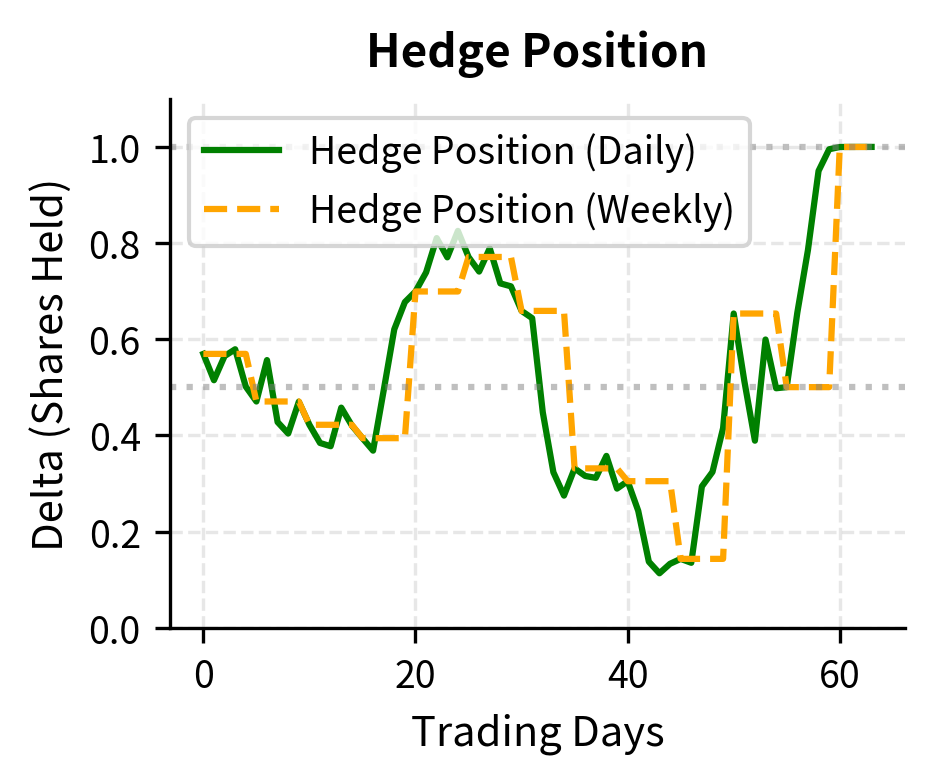
The simulation illustrates that more frequent rebalancing generally produces hedging P&L closer to the theoretical option value, but in practice each rebalance incurs transaction costs that the simulation doesn't capture. The optimal rebalancing frequency depends on the tradeoff between hedging error (reduced by more frequent rebalancing) and transaction costs (increased by more frequent rebalancing). This tradeoff is a central concern for you and drives significant research into optimal hedging policies.

Key ParametersLink Copied

The key parameters for Delta Hedging form the foundation of dynamic hedging practice, connecting the theoretical Greeks to practical implementation decisions:

$\Delta$ (Delta): The rate of change of option price with respect to the underlying asset price, which defines the hedge quantity. For a short call position, you buy delta shares of stock to neutralize directional exposure. Delta ranges from 0 to 1 for calls (0 to -1 for puts), with at-the-money options having deltas near 0.5. As the option moves deeper in-the-money, delta approaches 1; as it moves further out-of-the-money, delta approaches 0. This variation in delta is precisely what necessitates dynamic hedging.
Rebalancing Frequency: How often the hedge is adjusted, representing a critical implementation choice. More frequent rebalancing reduces tracking error, meaning the deviation between the hedge portfolio's value and the option liability, but increases transaction costs. Most market makers rebalance at least daily, with some adjusting intraday during volatile periods. The optimal frequency depends on transaction costs, position gamma, and your risk tolerance.
$\Gamma$ (Gamma): The rate of change of Delta with respect to the underlying price, which determines how quickly the hedge becomes stale after price movements. High gamma requires more frequent rebalancing because delta changes rapidly, while low gamma positions remain approximately neutral for longer. Gamma is highest for at-the-money options near expiration, making these positions the most challenging to hedge precisely.
$\sigma$ : Volatility of the underlying asset, which affects both the option price and all the Greeks used for hedging. Higher volatility increases option value, increases delta sensitivity (for out-of-the-money options), and generally increases the frequency of rebalancing required. Volatility also affects hedging P&L through the "gamma-theta" relationship: long gamma positions profit from realized volatility exceeding implied, while short gamma positions profit from the reverse.

Diversification as Risk ManagementLink Copied

While derivatives provide targeted hedging, diversification remains a fundamental risk management tool. Building on Modern Portfolio Theory from Part IV, effective diversification requires understanding correlation structures and how they change under stress.

The key insight is that correlations are not constant. Assets that appear uncorrelated in normal markets often become highly correlated during crises, precisely when diversification benefits are most needed. This phenomenon, sometimes called "correlation breakdown," makes naive diversification less effective than theory suggests.

We address this through:

Stress testing diversification benefits under crisis scenarios
Tail dependency analysis using copulas to model joint extreme movements
Dynamic correlation models that capture regime changes
Factor-based diversification across risk factors rather than just assets

Organizational Structure for Risk ManagementLink Copied

Effective risk management requires clear organizational accountability. The sophistication of risk analytics means little if decision rights are unclear or if risk warnings get ignored.

The Chief Risk Officer RoleLink Copied

The Chief Risk Officer (CRO) serves as the firm's primary advocate for prudent risk-taking. The CRO's responsibilities span:

Risk measurement and reporting: Ensuring the firm has appropriate models and metrics for all material risks, and that risk information reaches decision-makers in timely, understandable formats.

Limit setting and monitoring: Working with business leaders and the board to establish risk limits aligned with risk appetite, and monitoring compliance with those limits.

Risk policy development: Creating policies that govern risk-taking activities, including model validation standards, limit breach protocols, and new product approval processes.

Independent oversight: Providing a check on business units' natural tendency to underestimate risks in pursuit of profits. The CRO must have sufficient authority and independence to challenge traders and business leaders.

Board communication: Translating complex risk information into strategic insights for board-level discussions. The CRO helps the board understand the firm's risk profile and how it relates to strategic objectives.

CRO Independence

A critical success factor for the CRO role is independence from revenue-generating activities. The CRO should report directly to the CEO or board, not to business unit heads whose compensation depends on risk-taking. This organizational positioning allows the CRO to raise concerns without fear of retaliation and ensures risk considerations receive appropriate weight in business decisions.

Risk CommitteesLink Copied

Formal committees provide structured oversight of risk-taking and ensure diverse perspectives inform risk decisions.

Board Risk Committee: A subset of the board of directors (often with independent directors) that oversees enterprise risk management at the highest level. This committee:

Approves the firm's overall risk appetite framework
Reviews significant risk exposures and limit utilizations
Monitors emerging risks and risk trends
Evaluates the effectiveness of risk management processes
Ensures the CRO has adequate resources and authority

Management Risk Committee: Senior executives who meet regularly (often weekly) to review current risks and make operational decisions. This committee:

Reviews daily and weekly risk reports
Approves exceptions to risk limits
Decides on hedging strategies
Evaluates new products or strategies from a risk perspective
Coordinates risk management across business units

Asset-Liability Committee (ALCO): For banks and insurance companies, this committee specifically manages the mismatch between asset and liability characteristics, focusing on interest rate risk, liquidity risk, and capital management.

Model Risk Committee: Reviews and approves risk models before use, monitors model performance, and ensures appropriate model governance.

In[18]:

Code

@dataclass
class RiskCommitteeReport:
    """Structure for weekly risk committee reporting."""

    report_date: datetime
    firm_var_utilization: float  # Percent of firm VaR limit used
    desk_limit_breaches: List[Dict]
    largest_exposures: List[Dict]
    stress_test_results: Dict[str, float]
    emerging_risks: List[str]
    actions_required: List[str]

    def generate_summary(self) -> str:
        """Generate executive summary for risk committee."""
        summary = []

        # VaR utilization status
        if self.firm_var_utilization > 90:
            var_status = "ELEVATED"
        elif self.firm_var_utilization > 75:
            var_status = "MODERATE"
        else:
            var_status = "NORMAL"

        summary.append(f"Overall Risk Status: {var_status}")
        summary.append(
            f"Firm VaR Utilization: {self.firm_var_utilization:.1f}%"
        )
        summary.append(
            f"Limit Breaches This Week: {len(self.desk_limit_breaches)}"
        )

        if self.desk_limit_breaches:
            summary.append("\nLimit Breaches:")
            for breach in self.desk_limit_breaches:
                summary.append(
                    f"  - {breach['desk']}: {breach['limit_type']} "
                    f"({breach['utilization']:.0f}% utilization)"
                )

        summary.append("\nStress Test Results (Potential Losses):")
        for scenario, loss in self.stress_test_results.items():
            summary.append(f"  - {scenario}: ${loss / 1e6:.1f}M")

        if self.actions_required:
            summary.append("\nActions Required:")
            for action in self.actions_required:
                summary.append(f"  - {action}")

        return "\n".join(summary)

@dataclass
class RiskCommitteeReport:
    """Structure for weekly risk committee reporting."""

    report_date: datetime
    firm_var_utilization: float  # Percent of firm VaR limit used
    desk_limit_breaches: List[Dict]
    largest_exposures: List[Dict]
    stress_test_results: Dict[str, float]
    emerging_risks: List[str]
    actions_required: List[str]

    def generate_summary(self) -> str:
        """Generate executive summary for risk committee."""
        summary = []

        # VaR utilization status
        if self.firm_var_utilization > 90:
            var_status = "ELEVATED"
        elif self.firm_var_utilization > 75:
            var_status = "MODERATE"
        else:
            var_status = "NORMAL"

        summary.append(f"Overall Risk Status: {var_status}")
        summary.append(
            f"Firm VaR Utilization: {self.firm_var_utilization:.1f}%"
        )
        summary.append(
            f"Limit Breaches This Week: {len(self.desk_limit_breaches)}"
        )

        if self.desk_limit_breaches:
            summary.append("\nLimit Breaches:")
            for breach in self.desk_limit_breaches:
                summary.append(
                    f"  - {breach['desk']}: {breach['limit_type']} "
                    f"({breach['utilization']:.0f}% utilization)"
                )

        summary.append("\nStress Test Results (Potential Losses):")
        for scenario, loss in self.stress_test_results.items():
            summary.append(f"  - {scenario}: ${loss / 1e6:.1f}M")

        if self.actions_required:
            summary.append("\nActions Required:")
            for action in self.actions_required:
                summary.append(f"  - {action}")

        return "\n".join(summary)

In[19]:

Code

# Create sample weekly risk committee report
report = RiskCommitteeReport(
    report_date=datetime.now(),
    firm_var_utilization=82.5,
    desk_limit_breaches=[
        {
            "desk": "Credit Trading",
            "limit_type": "Sector Concentration",
            "utilization": 108,
        },
        {"desk": "Rates", "limit_type": "DV01", "utilization": 102},
    ],
    largest_exposures=[
        {"name": "US Equity Market", "exposure": 150_000_000},
        {"name": "EUR Interest Rates", "exposure": 85_000_000},
        {"name": "Credit Spreads", "exposure": 65_000_000},
    ],
    stress_test_results={
        "2008 Crisis Replay": 45_000_000,
        "Interest Rate +200bp": 28_000_000,
        "Credit Spread +100bp": 35_000_000,
        "Equity -20%": 32_000_000,
    },
    emerging_risks=[
        "Increased correlation between equity and credit exposures",
        "Liquidity deterioration in corporate bond markets",
    ],
    actions_required=[
        "Credit Trading to reduce sector concentration by EOD Friday",
        "Rates desk to present DV01 reduction plan to CRO",
    ],
)

# Create sample weekly risk committee report
report = RiskCommitteeReport(
    report_date=datetime.now(),
    firm_var_utilization=82.5,
    desk_limit_breaches=[
        {
            "desk": "Credit Trading",
            "limit_type": "Sector Concentration",
            "utilization": 108,
        },
        {"desk": "Rates", "limit_type": "DV01", "utilization": 102},
    ],
    largest_exposures=[
        {"name": "US Equity Market", "exposure": 150_000_000},
        {"name": "EUR Interest Rates", "exposure": 85_000_000},
        {"name": "Credit Spreads", "exposure": 65_000_000},
    ],
    stress_test_results={
        "2008 Crisis Replay": 45_000_000,
        "Interest Rate +200bp": 28_000_000,
        "Credit Spread +100bp": 35_000_000,
        "Equity -20%": 32_000_000,
    },
    emerging_risks=[
        "Increased correlation between equity and credit exposures",
        "Liquidity deterioration in corporate bond markets",
    ],
    actions_required=[
        "Credit Trading to reduce sector concentration by EOD Friday",
        "Rates desk to present DV01 reduction plan to CRO",
    ],
)

Out[20]:

Console

WEEKLY RISK COMMITTEE REPORT
============================================================
Report Date: 2026-01-25

Overall Risk Status: MODERATE
Firm VaR Utilization: 82.5%
Limit Breaches This Week: 2

Limit Breaches:
  - Credit Trading: Sector Concentration (108% utilization)
  - Rates: DV01 (102% utilization)

Stress Test Results (Potential Losses):
  - 2008 Crisis Replay: $45.0M
  - Interest Rate +200bp: $28.0M
  - Credit Spread +100bp: $35.0M
  - Equity -20%: $32.0M

Actions Required:
  - Credit Trading to reduce sector concentration by EOD Friday
  - Rates desk to present DV01 reduction plan to CRO

Out[21]:

Visualization

Stress test results showing potential losses under four adverse scenarios. The 2008 Crisis Replay scenario poses the largest risk at $45M potential loss, highlighting the importance of maintaining adequate capital buffers for tail events.

The weekly report highlights governance in action. While the firm-wide VaR utilization of 82.5% remains in the "Moderate" zone, specific breaches in Credit Trading (108%) and Rates (102%) trigger mandatory reduction plans. This demonstrates how the committee structure prevents desk-level excesses from compounding into firm-level threats.

Regulatory Influence on Risk ManagementLink Copied

Regulatory requirements significantly shape risk management practices, particularly for banks, broker-dealers, and insurance companies. Even firms outside direct regulatory oversight often adopt regulatory-inspired practices to satisfy institutional investors and maintain operational discipline.

Basel Framework for BanksLink Copied

The Basel Accords establish international standards for bank capital adequacy, stress testing, and market discipline. Building on our discussion of regulatory frameworks in the Overview chapter, the key requirements influencing risk management include:

Minimum capital ratios require banks to hold capital proportional to their risk-weighted assets. The three pillars of Basel III establish:

Pillar 1: Minimum capital requirements based on standardized risk weights or internal models
Pillar 2: Supervisory review requiring banks to assess their own capital adequacy beyond Pillar 1 minimums
Pillar 3: Market discipline through public disclosure of risk exposures and capital adequacy

Internal Models Approach (IMA) allows sophisticated banks to use their own VaR models for market risk capital, subject to regulatory approval and ongoing validation. Requirements include:

Daily VaR calculation at 99% confidence
Backtesting comparing VaR predictions to actual P&L
Stressed VaR based on a continuous 12-month period of financial stress
Multipliers that increase capital charges when models underperform

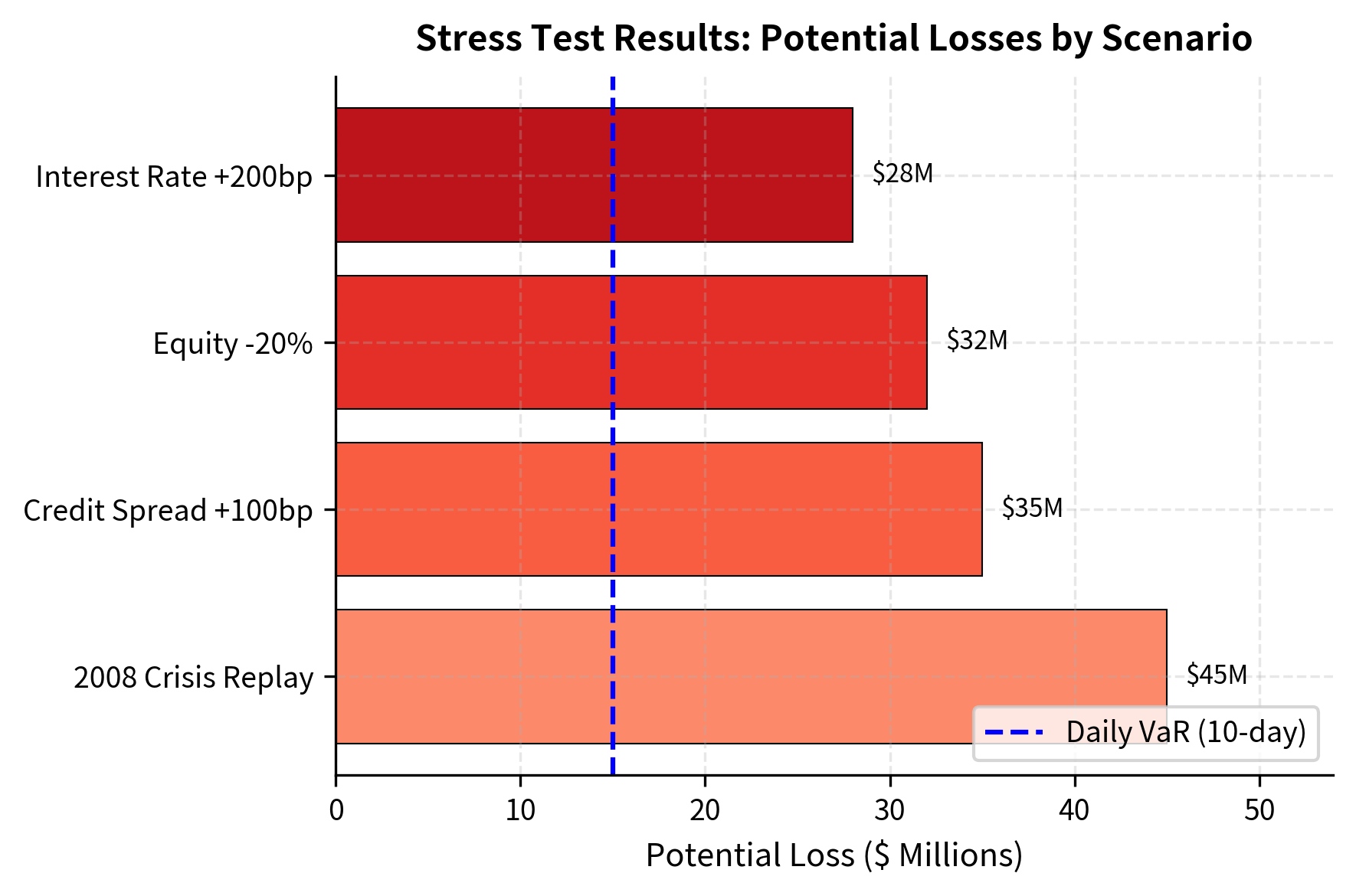
Stress testing requirements under CCAR (Comprehensive Capital Analysis and Review) and DFAST (Dodd-Frank Act Stress Tests) require large banks to demonstrate capital adequacy under severely adverse scenarios.

The Basel framework for market risk capital serves as the practical application of the theoretical concepts we have developed throughout Part V. At its core, the framework requires banks to hold capital reserves sufficient to absorb potential trading losses, with the capital amount determined by a combination of VaR-based measures and stress testing. The calculation explicitly recognizes that models may underestimate risk, incorporating multipliers that create a buffer between model-predicted losses and required capital.

The capital requirement combines two distinct VaR measures, each capturing a different aspect of market risk. The first component uses the bank's standard VaR model, reflecting the risk characteristics of the current portfolio under recent market conditions. The second component, Stressed VaR, applies the same model methodology to a historical period of significant market turbulence. By including both measures, the framework ensures capital adequacy both in normal markets and during crisis periods similar to past stress events.

In[22]:

Code

def calculate_market_risk_capital(
    var_99: float,
    stressed_var: float,
    multiplier: float = 3.0,
    stress_multiplier: float = 3.0,
) -> dict:
    """
    Calculate market risk capital under Basel framework.

    Parameters
    ----------
    var_99 : float
        10-day 99% VaR
    stressed_var : float
        10-day 99% stressed VaR
    stress_multiplier : float
        Regulatory multiplier for stressed VaR

    Returns
    -------
    dict
        Capital requirements breakdown
    """
    var_capital = multiplier * var_99
    stressed_var_capital = stress_multiplier * stressed_var
    total_capital = var_capital + stressed_var_capital

    return {
        "var_99_10day": var_99,
        "stressed_var_10day": stressed_var,
        "var_multiplier": multiplier,
        "stressed_var_multiplier": stress_multiplier,
        "var_capital_charge": var_capital,
        "stressed_var_capital_charge": stressed_var_capital,
        "total_market_risk_capital": total_capital,
    }


# Example capital calculation
var_99_1day = 15_000_000  # $15M daily VaR
var_99_10day = var_99_1day * np.sqrt(10)  # Scale to 10-day

stressed_var_1day = 28_000_000  # Higher during stress periods
stressed_var_10day = stressed_var_1day * np.sqrt(10)

capital_req = calculate_market_risk_capital(var_99_10day, stressed_var_10day)

def calculate_market_risk_capital(
    var_99: float,
    stressed_var: float,
    multiplier: float = 3.0,
    stress_multiplier: float = 3.0,
) -> dict:
    """
    Calculate market risk capital under Basel framework.

    Parameters
    ----------
    var_99 : float
        10-day 99% VaR
    stressed_var : float
        10-day 99% stressed VaR
    stress_multiplier : float
        Regulatory multiplier for stressed VaR

    Returns
    -------
    dict
        Capital requirements breakdown
    """
    var_capital = multiplier * var_99
    stressed_var_capital = stress_multiplier * stressed_var
    total_capital = var_capital + stressed_var_capital

    return {
        "var_99_10day": var_99,
        "stressed_var_10day": stressed_var,
        "var_multiplier": multiplier,
        "stressed_var_multiplier": stress_multiplier,
        "var_capital_charge": var_capital,
        "stressed_var_capital_charge": stressed_var_capital,
        "total_market_risk_capital": total_capital,
    }


# Example capital calculation
var_99_1day = 15_000_000  # $15M daily VaR
var_99_10day = var_99_1day * np.sqrt(10)  # Scale to 10-day

stressed_var_1day = 28_000_000  # Higher during stress periods
stressed_var_10day = stressed_var_1day * np.sqrt(10)

capital_req = calculate_market_risk_capital(var_99_10day, stressed_var_10day)

Out[23]:

Console

Market Risk Capital Calculation (Basel III)
==================================================
10-day 99% VaR: $47.4M
10-day 99% Stressed VaR: $88.5M

VaR multiplier: 3.0x
Stressed VaR multiplier: 3.0x

VaR capital charge: $142.3M
Stressed VaR capital charge: $265.6M

Total market risk capital: $407.9M

Out[24]:

Visualization

Basel III market risk capital components. The waterfall chart breaks down the total capital requirement into its constituent parts, highlighting the significant impact of the 3x regulatory multipliers.

Out[25]:

Visualization

Composition of Basel III market risk capital. Stressed VaR accounts for the majority (62%) of the capital requirement, reflecting the higher volatility assumptions used for crisis periods.

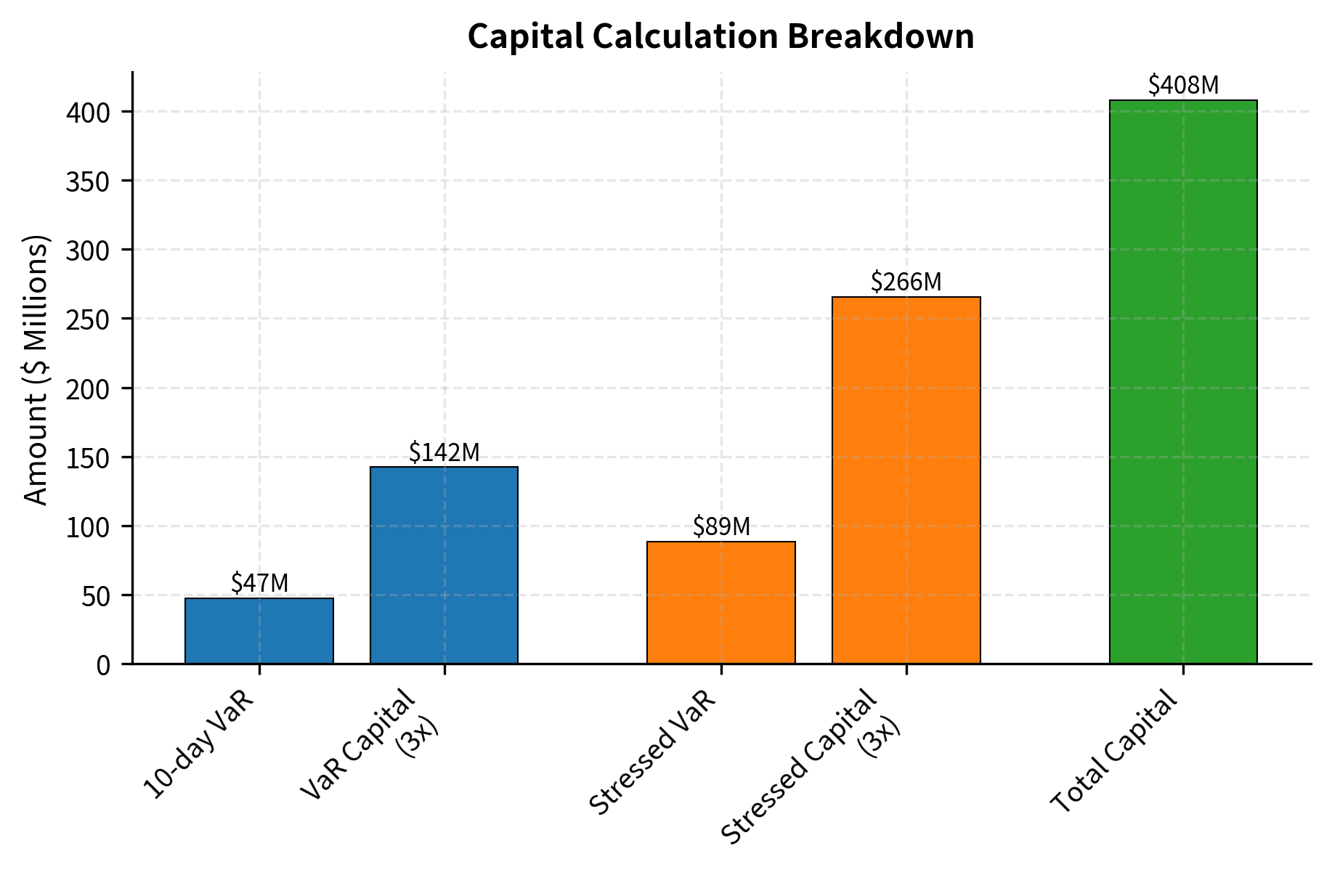
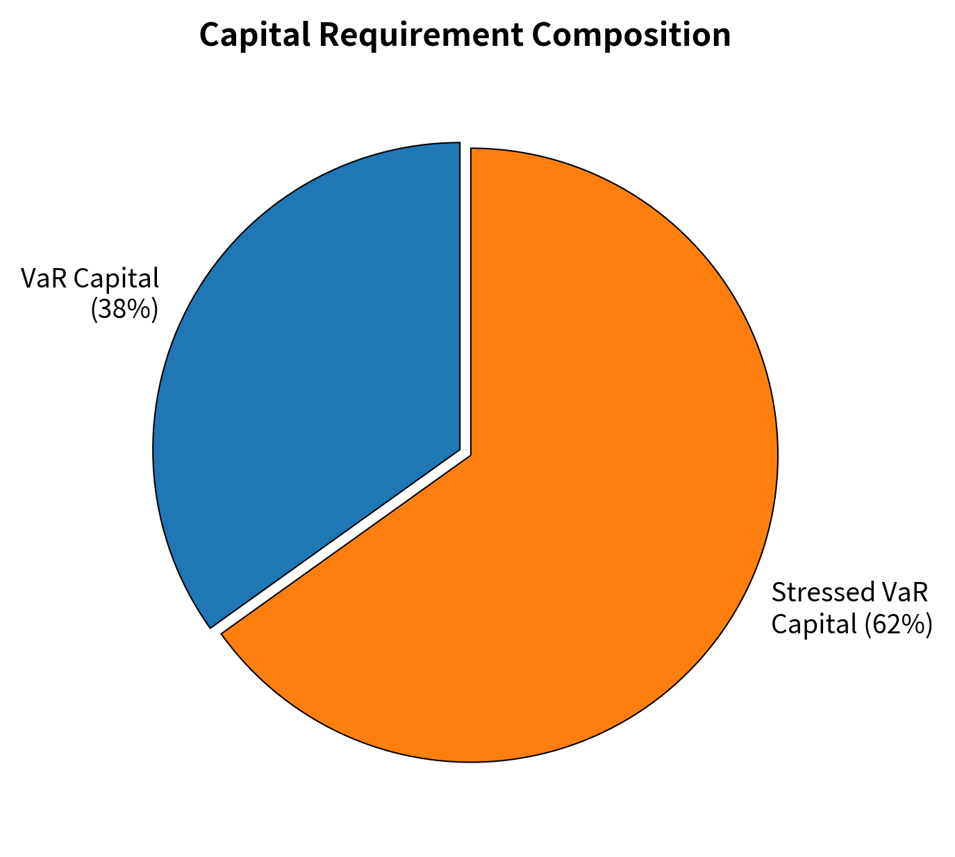
The calculation illustrates the punitive nature of the Basel framework for risky portfolios. The Stressed VaR component, derived from a historical crisis period, significantly increases the capital requirement because it captures the elevated losses that occur during market dislocations. With the regulatory multipliers set at 3.0, the firm must hold capital equal to three times its potential 10-day losses under each scenario. This threefold multiplier reflects regulatory conservatism, acknowledging that VaR models tend to underestimate extreme risks. The combined effect creates a substantial hurdle rate for trading activities, meaning that each trade must generate sufficient return to compensate for the capital it consumes.

Key ParametersLink Copied

The key parameters for Basel Market Risk Capital translate regulatory requirements into quantitative capital charges, creating the link between risk measurement and required financial resources:

VaR: Value-at-Risk calculated at 99% confidence over a 10-day horizon, representing potential loss in normal markets. The 10-day horizon reflects the assumption that, under stress, liquidating a trading portfolio may require more time than a single day. The 99% confidence level means the actual loss should exceed the VaR estimate on approximately one trading day per year (roughly 2.5 days out of 250). This parameter uses the bank's standard VaR model calibrated to recent market data, typically with an observation period of one year or longer.
Stressed VaR: VaR calculated using the same methodology but calibrated to historical data from a period of significant financial stress. Regulators require banks to identify a continuous 12-month period during which the bank's portfolio would have experienced significant losses, such as the 2008 financial crisis for most portfolios. This stressed calibration captures tail risks that may not be evident in recent market data, particularly during extended periods of low volatility.
Multipliers ( $m_c$ , $m_s$ ): Regulatory factors applied to VaR estimates, with a minimum value of 3.0 for both standard and stressed VaR. These multipliers can increase based on backtesting performance, meaning if the VaR model produces more exceptions than expected, the multiplier rises. The multipliers also incorporate qualitative factors assessed during regulatory examination, including model documentation, validation processes, and internal controls. The multiplicative structure creates strong incentives for banks to invest in model accuracy and robust risk infrastructure.

Best Practices for Non-Regulated EntitiesLink Copied

Hedge funds and proprietary trading firms often operate outside direct regulatory oversight, yet many voluntarily adopt robust risk management practices. Several factors drive this adoption:

Institutional investor requirements: Pension funds, endowments, and other institutional investors perform extensive due diligence before allocating to alternative managers. They often require:

Independent risk measurement (not performed by portfolio managers)
Regular risk reporting in standardized formats
Documented risk limits and breach procedures
Stress testing programs
Disaster recovery and business continuity plans

Prime broker risk limits: Prime brokers (banks that provide financing and clearing to hedge funds) impose risk limits on their hedge fund clients. Funds exceeding these limits face margin calls or reduced financing.

Operational due diligence: Institutional investors increasingly focus on operational infrastructure, including risk management technology and personnel, as predictor of manager quality.

Self-preservation: Perhaps most importantly, sound risk management protects the firm's own capital and reputation. High-profile hedge fund blowups like Long-Term Capital Management (1998) and Archegos (2021) demonstrate the consequences of inadequate risk management.

The Risk Management Feedback LoopLink Copied

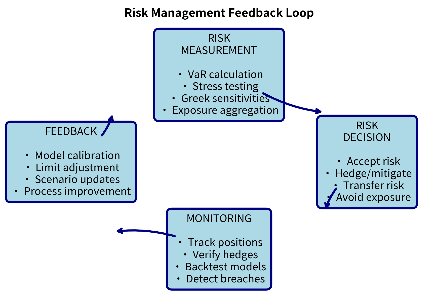
Effective risk management is not a one-time exercise but a continuous cycle of measurement, decision-making, and monitoring. Each stage feeds into the next, creating a system that learns and adapts.

The Cycle in PracticeLink Copied

The risk management process operates as a continuous loop with four interconnected stages. Understanding this cyclical nature is essential because it reveals that risk management is never "complete." Instead, it represents an ongoing dialogue between measurement, action, observation, and refinement.

Risk Measurement produces quantitative assessments of current exposures. This stage involves running the analytical models developed throughout this book, including VaR calculations, stress tests, sensitivity analyses, and exposure aggregations. The measurement function answers the question "where do we stand?" and provides the raw material for decision-making. Key outputs include:

Daily VaR and stress test calculations
Position-level Greeks and sensitivities
Counterparty exposure aggregation
Liquidity risk metrics

Risk Decision translates measurements into actions, bridging the gap between analytics and operational reality. Decision-makers, informed by the measurement outputs, must choose among several possible responses to any given risk:

Accept the risk as within appetite
Mitigate through hedging or position reduction
Transfer through insurance or derivatives
Avoid by declining to enter a position

Monitoring tracks both the risks themselves and the effectiveness of decisions made in response to measurements. This stage asks "did our actions work as intended?" and "have conditions changed since our last assessment?" Monitoring creates accountability and early warning capability:

Did hedges perform as expected?
Were risk estimates accurate (backtesting)?
Are new risks emerging?
Are limits still appropriate?

Feedback incorporates lessons into improved measurement and decisions, closing the loop and enabling organizational learning. Without explicit feedback mechanisms, the same mistakes recur and opportunities for improvement remain unrealized:

Calibrate models based on realized outcomes
Adjust limits based on business needs and market conditions
Update stress scenarios based on emerging risks
Refine hedging strategies based on effectiveness analysis

Out[26]:

Visualization

Circular flow diagram showing four stages: Risk Measurement, Risk Decision, Monitoring, and Feedback connecting in a continuous loop. — The risk management feedback loop showing the continuous cycle from measurement through decision and monitoring back to improved measurement. Each stage generates information that improves the next iteration.

Backtesting and Model ValidationLink Copied

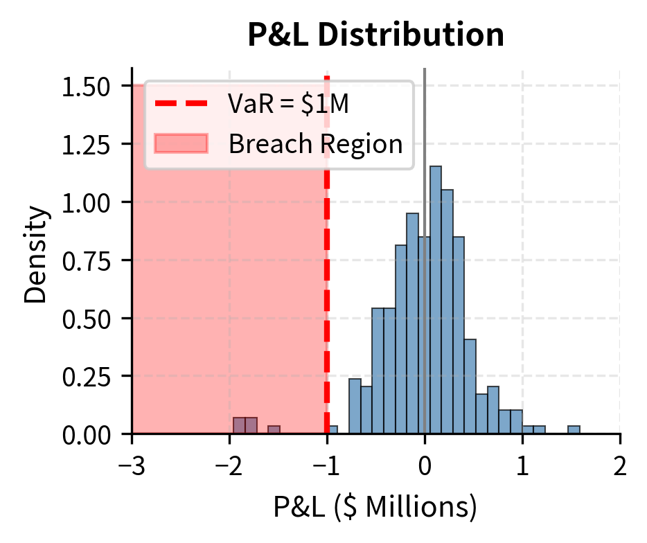
Backtesting compares risk model predictions to realized outcomes, serving as the primary mechanism for validating model accuracy. The concept is straightforward: if a model predicts that losses should exceed a certain threshold with a specific probability, we can compare this prediction against actual experience. For VaR models, this typically involves counting how often actual losses exceed the VaR estimate and comparing this frequency to the theoretical expectation.

The statistical foundations of backtesting connect directly to the confidence level interpretation of VaR. A 99% VaR predicts that losses will exceed the threshold on approximately 1% of days, or about 2.5 days per year for a 250-day trading year. If actual breaches occur significantly more or less frequently, the model may be miscalibrated. The challenge lies in distinguishing genuine model failures from random variation, since small sample sizes make statistical inference difficult.

The Kupiec test provides a formal statistical framework for this assessment. It constructs a likelihood ratio statistic comparing the probability of observing the actual number of breaches under the model's assumed accuracy versus under the observed breach rate. Large values of this statistic indicate that the observed breach rate is statistically inconsistent with the model's claims, suggesting model inadequacy.

In[27]:

Code

def backtest_var(
    var_forecasts: np.ndarray,
    actual_pnl: np.ndarray,
    confidence_level: float = 0.99,
) -> dict:
    """
    Backtest VaR model by comparing forecasts to realized P&L.

    Parameters
    ----------
    var_forecasts : np.ndarray
        Daily VaR forecasts (positive values representing loss threshold)
    actual_pnl : np.ndarray
        Realized daily P&L
    confidence_level : float
        VaR confidence level

    Returns
    -------
    dict
        Backtesting statistics
    """
    n_days = len(actual_pnl)

    # VaR breach occurs when actual loss exceeds VaR forecast
    breaches = actual_pnl < -var_forecasts
    n_breaches = breaches.sum()
    breach_rate = n_breaches / n_days

    # Expected breach rate
    expected_rate = 1 - confidence_level
    expected_breaches = expected_rate * n_days

    # Kupiec test statistic (likelihood ratio test)
    if n_breaches > 0 and n_breaches < n_days:
        log_lik_null = n_breaches * np.log(expected_rate) + (
            n_days - n_breaches
        ) * np.log(1 - expected_rate)
        log_lik_alt = n_breaches * np.log(breach_rate) + (
            n_days - n_breaches
        ) * np.log(1 - breach_rate)
        lr_stat = -2 * (log_lik_null - log_lik_alt)
    else:
        lr_stat = np.nan

    # Basel traffic light zones
    if n_breaches <= 4:
        zone = "GREEN"
    elif n_breaches <= 9:
        zone = "YELLOW"
    else:
        zone = "RED"

    return {
        "n_days": n_days,
        "n_breaches": n_breaches,
        "breach_rate": breach_rate,
        "expected_rate": expected_rate,
        "expected_breaches": expected_breaches,
        "kupiec_lr_stat": lr_stat,
        "basel_zone": zone,
        "breaches": breaches,
    }


# Simulate VaR backtesting scenario
np.random.seed(42)
n_days = 250  # One trading year

# Generate VaR forecasts (assuming constant $1M VaR)
var_forecasts = np.ones(n_days) * 1_000_000

# Generate P&L with occasional large losses
actual_pnl = np.random.normal(50_000, 400_000, n_days)

# Add a few stress events
stress_days = np.random.choice(n_days, size=5, replace=False)
actual_pnl[stress_days] = np.random.uniform(-1_500_000, -2_500_000, 5)

backtest_results = backtest_var(
    var_forecasts, actual_pnl, confidence_level=0.99
)

def backtest_var(
    var_forecasts: np.ndarray,
    actual_pnl: np.ndarray,
    confidence_level: float = 0.99,
) -> dict:
    """
    Backtest VaR model by comparing forecasts to realized P&L.

    Parameters
    ----------
    var_forecasts : np.ndarray
        Daily VaR forecasts (positive values representing loss threshold)
    actual_pnl : np.ndarray
        Realized daily P&L
    confidence_level : float
        VaR confidence level

    Returns
    -------
    dict
        Backtesting statistics
    """
    n_days = len(actual_pnl)

    # VaR breach occurs when actual loss exceeds VaR forecast
    breaches = actual_pnl < -var_forecasts
    n_breaches = breaches.sum()
    breach_rate = n_breaches / n_days

    # Expected breach rate
    expected_rate = 1 - confidence_level
    expected_breaches = expected_rate * n_days

    # Kupiec test statistic (likelihood ratio test)
    if n_breaches > 0 and n_breaches < n_days:
        log_lik_null = n_breaches * np.log(expected_rate) + (
            n_days - n_breaches
        ) * np.log(1 - expected_rate)
        log_lik_alt = n_breaches * np.log(breach_rate) + (
            n_days - n_breaches
        ) * np.log(1 - breach_rate)
        lr_stat = -2 * (log_lik_null - log_lik_alt)
    else:
        lr_stat = np.nan

    # Basel traffic light zones
    if n_breaches <= 4:
        zone = "GREEN"
    elif n_breaches <= 9:
        zone = "YELLOW"
    else:
        zone = "RED"

    return {
        "n_days": n_days,
        "n_breaches": n_breaches,
        "breach_rate": breach_rate,
        "expected_rate": expected_rate,
        "expected_breaches": expected_breaches,
        "kupiec_lr_stat": lr_stat,
        "basel_zone": zone,
        "breaches": breaches,
    }


# Simulate VaR backtesting scenario
np.random.seed(42)
n_days = 250  # One trading year

# Generate VaR forecasts (assuming constant $1M VaR)
var_forecasts = np.ones(n_days) * 1_000_000

# Generate P&L with occasional large losses
actual_pnl = np.random.normal(50_000, 400_000, n_days)

# Add a few stress events
stress_days = np.random.choice(n_days, size=5, replace=False)
actual_pnl[stress_days] = np.random.uniform(-1_500_000, -2_500_000, 5)

backtest_results = backtest_var(
    var_forecasts, actual_pnl, confidence_level=0.99
)

Out[28]:

Console

VaR Backtesting Results
==================================================
Observation period: 250 trading days
Number of VaR breaches: 5
Actual breach rate: 2.00%
Expected breach rate (99% VaR): 1.00%
Expected breaches: 2.5
Kupiec LR statistic: 1.96

Basel Traffic Light Zone: YELLOW
  → Potential model weakness, investigation warranted

Out[29]:

Visualization

Daily P&L versus VaR threshold (dashed red line) over one year. Five breaches occur during the period, shown as red dots, placing the model performance in the Basel yellow zone.

Distribution of Daily P&L relative to the VaR threshold. The histogram shows a heavy left tail where realized losses exceed the 1M USD VaR estimate, visually representing the model's 99% confidence boundary.

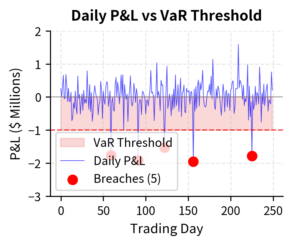
The backtesting framework provides quantitative evidence of model performance that informs both regulatory capital calculations and internal model improvement efforts. Under Basel guidelines, the "traffic light" approach creates a practical categorization system: 0-4 breaches in a year places the model in the "green zone" with no penalty, 5-9 breaches moves the model into the "yellow zone" requiring investigation and potentially triggering capital multiplier increases, while 10 or more breaches triggers the "red zone" with mandatory and substantial capital multiplier increases. This regulatory structure creates strong incentives for accurate model calibration.

Key ParametersLink Copied

The key parameters for VaR Backtesting connect statistical theory to practical model validation, providing the foundation for assessing whether risk models perform as intended:

Confidence Level: The probability level of the VaR model, typically 99% for regulatory purposes. This parameter determines the expected breach rate against which actual performance is compared. At 99% confidence, the model predicts losses will exceed VaR on approximately 1% of days. The choice of confidence level involves a tradeoff: higher confidence levels provide greater protection against extreme losses but are more difficult to validate statistically because exceptions are rare events.
$N$ : Number of observations in the backtesting period, typically 250 trading days representing one year. Longer observation periods provide more statistical power to detect model deficiencies but may include regime changes that complicate interpretation. The minimum observation period for regulatory backtesting is typically one year, though internal validation may use longer histories.
Breaches: The count of days where actual loss exceeded the VaR forecast, representing the primary outcome variable for backtesting. Too few breaches suggest the VaR estimate is overly conservative, potentially causing inefficient capital allocation. Too many breaches indicate the model underestimates risk, leaving the firm exposed to larger losses than anticipated. The expected number of breaches equals $(1 - \text{confidence level}) \times N$ , or approximately 2.5 breaches per year at 99% confidence.
Kupiec Statistic: A likelihood ratio test statistic used to determine if the number of breaches is statistically consistent with the confidence level. The statistic follows a chi-squared distribution with one degree of freedom under the null hypothesis that the model is correctly calibrated. Values exceeding approximately 3.84 (the 95th percentile) suggest model misspecification at the 5% significance level. This formal statistical test complements the simpler breach-counting approach with rigorous hypothesis testing.

Building a Risk CultureLink Copied

Beyond formal structures and quantitative models, effective risk management requires a risk culture that permeates the organization. Culture determines whether employees raise concerns, whether risk considerations influence daily decisions, and whether the firm learns from near-misses.

Elements of Strong Risk CultureLink Copied

Strong risk culture depends on several interconnected elements:

Tone from the top: Senior leadership must visibly prioritize risk management. When executives routinely ask about risk implications of business decisions and publicly support the CRO, it signals that risk management is valued.
Open communication: Employees must feel safe raising concerns about risks or potential policy violations. Fear of retaliation or being labeled a "naysayer" suppresses valuable risk intelligence.
Clear accountability: Every significant risk should have an owner responsible for monitoring and managing it. Diffuse ownership leads to risks falling through the cracks.
Balanced incentives: Compensation structures that reward only revenue generation encourage excessive risk-taking. Including risk-adjusted metrics in performance evaluation aligns individual and firm interests.
Learning from mistakes: Post-mortems on both losses and near-misses extract lessons that improve future risk management. A culture that punishes all losses regardless of process quality discourages appropriate risk-taking.

Common Cultural FailuresLink Copied

Historical risk management failures often trace to cultural weaknesses rather than technical deficiencies:

Overconfidence in models: Long-Term Capital Management had Nobel laureates and sophisticated models but concentrated bets on mean reversion that failed spectacularly when correlations spiked during the 1998 Russian default.
Siloed risk management: The 2008 financial crisis revealed that many banks measured risks within individual business units but failed to aggregate exposures to see concentrations in mortgage-related securities across the enterprise.
Shooting the messenger: When risk managers who raise concerns are marginalized or terminated, organizations lose early warning capability. Several pre-crisis risk managers at major banks were sidelined for being "too negative."
Normalization of deviance: When small policy violations occur without consequences, larger violations gradually become acceptable. Limit breaches that go unenforced erode the entire limit framework's credibility.

Measuring Risk CultureLink Copied

While culture is qualitative, firms attempt to measure it through:

Risk culture surveys asking employees about their perception of risk management's importance and effectiveness
Escalation tracking counting how often concerns are raised and how they're resolved
Limit breach analysis examining patterns in breaches and enforcement actions
Near-miss reporting tracking events that could have caused losses but didn't
Training completion rates and assessment scores for risk education programs

Limitations and ChallengesLink Copied

Despite sophisticated tools and organizational structures, risk management faces inherent limitations that you must acknowledge.

Model risk is pervasive. All risk models simplify reality through assumptions about distributions, correlations, and market behavior. These assumptions often fail precisely when accuracy matters most: during market stress. The well-known limitations of VaR, including its inability to capture tail risk and its potential for gaming, apply to most quantitative risk measures. We should treat model outputs as inputs to judgment, not substitutes for it.

The illusion of precision can be dangerous. Reporting risk to many decimal places creates false confidence in measurement accuracy. A VaR number of $12,345,678 suggests precision that doesn't exist given the underlying assumptions and estimation uncertainty. You must communicate uncertainty around point estimates and help decision-makers understand the range of possible outcomes.

Incentive conflicts complicate implementation. Business units naturally resist constraints on their activities, and traders have strong incentives to characterize their positions as less risky than they may be. You must maintain healthy skepticism and verify claims independently. The challenge is maintaining constructive relationships with business units while preserving independence.

Emerging risks may not appear in historical data. Climate risk, cyber risk, and pandemic risk have limited historical precedent in financial markets, making traditional statistical approaches less reliable. Scenario analysis and expert judgment become essential complements to quantitative models.

Costs of risk management are certain while benefits are probabilistic. Firms pay for risk management infrastructure, hedging costs, and capital held against risk every day. The payoff (avoiding catastrophic losses) occurs only occasionally and counterfactually (what would have happened without risk management). This asymmetry creates pressure to reduce risk management expenditures, particularly when times are good.

SummaryLink Copied

This chapter has explored the practices and policies that translate risk measurement into risk control. The key takeaways are:

Risk limits provide concrete constraints on risk-taking. VaR limits, stop-loss limits, concentration limits, and Greek limits work together to control risk from multiple angles. Effective enforcement requires real-time monitoring, clear escalation procedures, and meaningful consequences for violations.

Hedging strategies require tradeoffs. Linear hedges with futures are simple but create basis risk. Options provide asymmetric protection but cost premium. Delta hedging requires continuous adjustment. Diversification helps but correlations increase during crises.

Organizational structure matters. The CRO must have independence and authority. Risk committees at board and management levels ensure proper oversight. Clear accountability for specific risks prevents gaps.

Regulation shapes practice even for non-regulated entities. Basel requirements for banks establish capital standards and stress testing expectations. Institutional investors demand similar rigor from hedge funds. Best practices diffuse across the industry.

Risk management is a continuous cycle. Measurement, decision, monitoring, and feedback form an iterative loop that enables learning and adaptation. Backtesting validates models and identifies needed improvements.

Culture determines effectiveness. The most sophisticated models fail if employees don't raise concerns, if incentives encourage excessive risk-taking, or if leadership doesn't prioritize risk. Building strong risk culture requires sustained attention to tone, communication, accountability, and learning.

As we transition to Part VI on quantitative trading strategies, you'll see how the risk management framework developed throughout Part V integrates with strategy design and implementation. The mean reversion, momentum, and factor strategies covered ahead all require careful risk management to survive the inevitable periods when markets move against them.

QuizLink Copied

Ready to test your understanding? Take this quick quiz to reinforce what you've learned about risk management practices and policies.

Loading component...

Comments

Back to Quantitative Finance

Previous Chapter

Liquidity Risk and Other Non-Market Risks

Next Chapter

Overview of Quantitative Trading Strategies

Reference

BIBTEXAcademic

@misc{riskmanagementpracticeslimitshedginggovernance, author = {Michael Brenndoerfer}, title = {Risk Management Practices: Limits, Hedging & Governance}, year = {2025}, url = {https://mbrenndoerfer.com/writing/risk-management-practices-policies-limits-hedging-governance}, organization = {mbrenndoerfer.com}, note = {Accessed: 2025-01-01} }

APAAcademic

Michael Brenndoerfer (2025). Risk Management Practices: Limits, Hedging & Governance. Retrieved from https://mbrenndoerfer.com/writing/risk-management-practices-policies-limits-hedging-governance

MLAAcademic

Michael Brenndoerfer. "Risk Management Practices: Limits, Hedging & Governance." 2026. Web. today. <https://mbrenndoerfer.com/writing/risk-management-practices-policies-limits-hedging-governance>.

CHICAGOAcademic

Michael Brenndoerfer. "Risk Management Practices: Limits, Hedging & Governance." Accessed today. https://mbrenndoerfer.com/writing/risk-management-practices-policies-limits-hedging-governance.

HARVARDAcademic

Michael Brenndoerfer (2025) 'Risk Management Practices: Limits, Hedging & Governance'. Available at: https://mbrenndoerfer.com/writing/risk-management-practices-policies-limits-hedging-governance (Accessed: today).

SimpleBasic

Michael Brenndoerfer (2025). Risk Management Practices: Limits, Hedging & Governance. https://mbrenndoerfer.com/writing/risk-management-practices-policies-limits-hedging-governance

Direct link:

https://mbrenndoerfer.com/writing/risk-management-practices-policies-limits-hedging-governance

About the author: Michael Brenndoerfer

All opinions expressed here are my own and do not reflect the views of my employer.

Michael currently works as an Associate Director of Data Science at EQT Partners in Singapore, leading AI and data initiatives across private capital investments.

With over a decade of experience spanning private equity, management consulting, and software engineering, he specializes in building and scaling analytics capabilities from the ground up. He has published research in leading AI conferences and holds expertise in machine learning, natural language processing, and value creation through data.

View Full Resume Publications Contact Books

Risk Management Practices: Limits, Hedging & Governance

Risk Management Practices and PoliciesLink Copied

Risk Limits and Enforcement MechanismsLink Copied

Types of Risk LimitsLink Copied

Limit Enforcement MechanismsLink Copied

Dynamic Limit AdjustmentLink Copied

Hedging Strategies in PracticeLink Copied

Hedging Objectives and TradeoffsLink Copied

Linear Hedging with Forwards and FuturesLink Copied

Key ParametersLink Copied

Options-Based Hedging StrategiesLink Copied

Key ParametersLink Copied

Delta Hedging for Options PortfoliosLink Copied

Key ParametersLink Copied

Diversification as Risk ManagementLink Copied

Organizational Structure for Risk ManagementLink Copied

The Chief Risk Officer RoleLink Copied

Risk CommitteesLink Copied

Regulatory Influence on Risk ManagementLink Copied

Basel Framework for BanksLink Copied

Key ParametersLink Copied

Best Practices for Non-Regulated EntitiesLink Copied

The Risk Management Feedback LoopLink Copied

The Cycle in PracticeLink Copied

Backtesting and Model ValidationLink Copied

Key ParametersLink Copied

Building a Risk CultureLink Copied

Elements of Strong Risk CultureLink Copied

Common Cultural FailuresLink Copied

Measuring Risk CultureLink Copied

Limitations and ChallengesLink Copied

SummaryLink Copied

QuizLink Copied

Comments

Reference

About the author: Michael Brenndoerfer

Related Content

Liquidity Risk Management: Beyond VaR and Market Risk

Counterparty Risk and CVA: Credit Valuation Adjustment

Credit Risk Modeling: Merton, Hazard Rates & Copulas

Stay updated

Comments

About the author: Michael Brenndoerfer

Related Content

Liquidity Risk Management: Beyond VaR and Market Risk

Counterparty Risk and CVA: Credit Valuation Adjustment

Credit Risk Modeling: Merton, Hazard Rates & Copulas

Stay updated