Quantitative Trading Strategies: Alpha, Backtesting & Performance

Quantitative trading represents a fundamental shift in how investment decisions are made: replacing human intuition with mathematical models, statistical analysis, and systematic rules. Rather than relying on subjective judgments about which stocks to buy or sell, you develop algorithms that identify patterns in data, generate trading signals, and execute positions according to predefined rules.

This approach has grown from a niche practice in the 1970s to a dominant force in modern finance. Today, quantitative and algorithmic strategies account for the majority of trading volume in equity markets, and systematic approaches have expanded into fixed income, commodities, currencies, and cryptocurrency markets. Finding a pattern that predicts future returns allows you to capture profits consistently while managing risk precisely.

But quantitative trading is far more than simply building a model and letting it run. The most challenging aspects involve distinguishing genuine predictive signals from statistical noise, avoiding the trap of overfitting historical data, and navigating the gap between backtested performance and live trading results. This chapter provides the conceptual foundation for understanding how quantitative strategies work, how they're developed, and how to evaluate whether a strategy is likely to succeed.

The concept of alpha sits at the heart of every quantitative trading strategy. To understand why alpha matters, consider a fundamental question: is performance the result of skill or simply a reward for taking on risk? This distinction is not merely academic. It determines whether a trading strategy offers something truly valuable or whether its returns could be replicated cheaply through passive exposure to market risk.

In Part IV, we explored how the Capital Asset Pricing Model decomposes expected returns into compensation for systematic risk (beta) and a residual component. This decomposition provides a powerful framework for separating skill from risk-taking. Alpha represents that residual, the returns that cannot be explained by exposure to market risk factors. When we observe a portfolio's returns, alpha answers the question: "What performance remains after we account for the systematic risks the portfolio was exposed to?"

The formula follows the CAPM framework from Part IV, Chapter 2. We can express an investment's excess return as the sum of its systematic risk exposure and the return that goes beyond this expectation. The regression equation is:

Each term in this equation plays a specific role in isolating alpha:

• $r_i$: return of investment $i$, the total performance we observe
• $r_f$: risk-free rate, the return available without any risk
• $r_m$: market return, representing the performance of the overall market
• $\beta_i$: sensitivity to market movements, measuring how much the investment rises or falls when the market moves
• $\beta_i(r_m - r_f)$: systematic return component explained by market risk. This term captures what the investment should have earned given how risky it is relative to the market. A high-beta investment should earn more than a low-beta investment in up markets, but this extra return is compensation for risk, not skill.
• $\alpha_i$: return component unexplained by market exposure. This is the residual, the performance that cannot be attributed to riding the market up or down.
• $\epsilon_i$: idiosyncratic error term, representing random noise unrelated to either systematic factors or persistent skill

By regressing an investment's excess returns against the market's excess returns, we are asking: "How much of this investment's performance came from market exposure, and how much came from something else?" The slope of this regression (beta) tells us the market exposure, the intercept (alpha) tells us the average return beyond what that exposure would predict.

A positive alpha of 3% annually means the investment delivered 3 percentage points more than what the CAPM predicts given its beta. This is economically significant because it represents genuine skill (or edge) rather than simply being rewarded for taking on market risk, something you can do by buying an index fund. You could achieve high returns simply by taking on more market risk, but such returns are not alpha. True alpha comes from doing something that others cannot easily replicate.

A single-factor CAPM is often insufficient, as discussed in Part IV, Chapter 3. The market factor alone does not capture all the systematic risks that drive returns. Over decades of research, academics and practitioners have identified additional factors, such as value, momentum, and size, that explain return patterns across securities. These factors represent systematic sources of risk that investors are compensated for bearing.

The natural extension is to use multi-factor models that account for these additional risk dimensions. By including more factors, we raise the bar for what counts as alpha, ensuring that we are measuring truly unexplained returns rather than returns that simply reflect exposure to well-known risk premia:

This equation generalizes the single-factor CAPM to accommodate any number of systematic factors. Each component has a clear interpretation:

• $r_i$: return of investment $i$
• $r_f$: risk-free rate
• $\alpha_i$: genuine alpha (unexplained return). In this multi-factor context, alpha is what remains after accounting for all systematic factors, not just the market.
• $\beta_{ij}$: sensitivity of investment $i$ to factor $j$. Each factor has its own beta, measuring the investment's exposure to that particular risk dimension.
• $f_j$: return of risk factor $j$ (e.g., value, momentum, size). These are the systematic risk premia that drive returns across all securities.
• $\sum_{j=1}^{k} \beta_{ij} f_j$: component of return explained by systematic risk factors. This sum represents the total return attributable to the investment's exposure across all k factors.
• $k$: number of risk factors included in the model
• $\epsilon_i$: residual error

Alpha in this framework is the return unexplained by any of the systematic factors. This is a higher bar to clear but a more meaningful measure of genuine edge. A strategy might appear to generate alpha against a single-factor model, but once we control for momentum or value exposure, that alpha might vanish entirely.

This distinction matters enormously for you. A strategy that appears to generate 10% annual returns might actually deliver zero alpha if those returns are entirely explained by exposure to the momentum factor. You could achieve the same momentum exposure by simply buying a momentum ETF, typically at lower cost and with less operational complexity. True alpha comes from finding inefficiencies that the standard factor models don't capture.

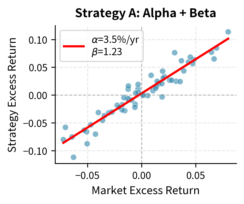
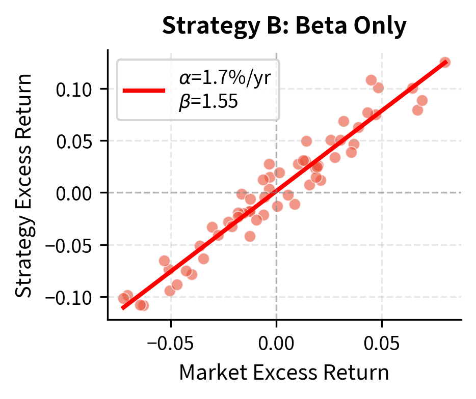
The regression analysis reveals the crucial distinction: Strategy A generates returns through genuine alpha, while Strategy B achieves similar absolute returns purely through higher market exposure. The practical implication is profound. An investor can replicate Strategy B's exposure cheaply by leveraging an index fund; Strategy A's alpha represents true value creation that cannot be easily replicated.

Key ParametersLink Copied

The key parameters for the alpha simulation are:

• alpha_a: Monthly excess return unexplained by market risk. Sets the "skill" level of the strategy. In our simulation, this represents the genuine edge that generates returns beyond what market exposure would predict.
• beta_a: Sensitivity to market movements. Determines how much the strategy moves with the market. Higher beta means more volatile returns that track the market more closely.

Alpha doesn't materialize from nothing. It emerges from exploiting market inefficiencies: situations where asset prices don't fully reflect available information. Understanding these sources helps you identify where to look for alpha and assess whether a discovered pattern represents a genuine opportunity or a statistical artifact. The main sources include:

• Informational advantages: Accessing or processing information faster or more effectively than other market participants
• Analytical advantages: Using superior models or analytical frameworks to extract signals from publicly available data
• Behavioral exploitation: Capitalizing on systematic biases in how other investors make decisions
• Structural inefficiencies: Exploiting constraints faced by other market participants, such as regulatory limits, benchmark tracking, or liquidity needs
• Risk transfer: Earning returns by providing insurance or liquidity to other market participants

The challenge is that alpha is a finite resource. When a strategy becomes widely known and adopted, the inefficiency it exploits tends to diminish or disappear entirely. This "alpha decay" means you must continuously evolve your approaches.

Quantitative strategies span an enormous range of approaches, timeframes, and market segments. Understanding these categories provides a framework for thinking about how different strategies work and what skills they require.

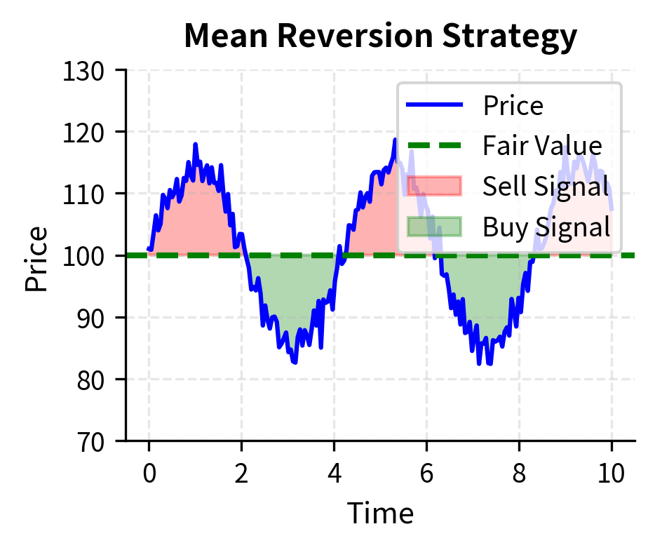
Statistical arbitrage strategies identify assets whose prices have diverged from their historical or predicted relationships, betting that prices will revert to normal levels. The classic example is pairs trading: if two historically correlated stocks diverge significantly, you short the outperformer and buy the underperformer, profiting when the relationship normalizes.

The core assumption underlying mean reversion strategies is that price deviations are temporary and driven by noise rather than fundamental changes. This works best in markets where:

• Assets have strong economic linkages (two oil companies, a stock and its ADR)
• Arbitrage mechanisms exist to enforce pricing relationships
• Deviations are caused by temporary factors like order flow imbalances

Mean reversion strategies typically have holding periods ranging from days to weeks and require sophisticated risk management because the assumption of reversion can fail catastrophically when regime changes occur.

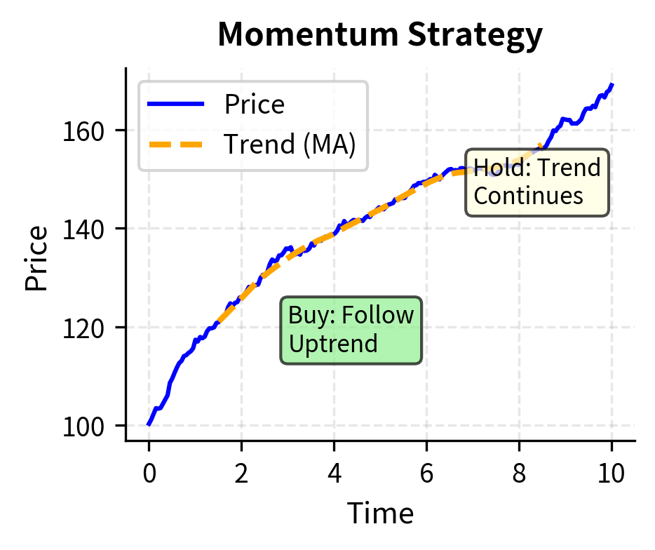
Trend following strategies take the opposite view: rather than betting on reversion, they bet that existing price trends will continue. As we observed in Part III, Chapter 1 on the stylized facts of financial returns, asset returns exhibit positive autocorrelation at medium-term horizons, a genuine anomaly that contradicts weak-form market efficiency.

Momentum strategies identify assets that have performed well (or poorly) over recent periods and bet that the trend continues. The economic explanations include:

• Underreaction: Investors initially underreact to new information, causing prices to adjust gradually
• Behavioral feedback: Rising prices attract more buyers, creating self-reinforcing cycles
• Risk-based explanations: Momentum returns may compensate for crash risk during trend reversals

Trend following strategies tend to have longer holding periods (weeks to months) and can be applied across asset classes. They also tend to perform well during market crises when trends become extreme, providing valuable diversification.

Factor investing systematically captures returns associated with characteristics like value, quality, momentum, and low volatility. As we discussed in Part IV, Chapter 3, these factors have historically delivered positive risk-adjusted returns.

Long/short equity strategies extend this concept by constructing portfolios that are long stocks with favorable factor exposures and short stocks with unfavorable exposures. The resulting portfolio has limited net market exposure but concentrated factor exposure, aiming to generate returns from stock selection rather than market direction.

Building on our coverage of factor models, a typical long/short equity portfolio might target a return structure that separates stock selection skill from market direction. The return of such a portfolio can be expressed as:

This equation reveals the multiple dimensions of return generation in a long/short strategy:

• $r_{\text{portfolio}}$: return of the strategy, the total performance we observe
• $\alpha$: excess return generated by stock selection. This is the value added by choosing specific stocks within each factor group.
• $\beta_{\text{market}}$: exposure to the broad market (targeted $\approx 0$). By maintaining near-zero market beta, the strategy aims to be immune to overall market direction.
• $r_{\text{market}}$: market return
• $\beta_{\text{value}}, \beta_{\text{momentum}}$: exposures to factor risk premia (targeted $> 0$). These positive exposures mean the strategy is intentionally harvesting the value and momentum premiums.
• $f_{\text{value}}, f_{\text{momentum}}$: returns of the value and momentum factors
• $\epsilon$: residual noise

Volatility strategies exploit discrepancies in how volatility is priced across instruments or time periods. As we explored extensively in Part III on options pricing, implied volatility often differs from realized volatility, and the volatility surface exhibits persistent patterns.

Common volatility strategies include:

• Variance risk premium harvesting: Selling options to capture the tendency for implied volatility to exceed realized volatility
• Volatility surface arbitrage: Exploiting inconsistencies across strikes and expirations
• Dispersion trading: Trading the relationship between index volatility and single-stock volatility

These strategies require deep understanding of options mechanics and the Greeks we covered in Part III, Chapter 7.

Market makers provide liquidity by continuously offering to buy and sell assets, earning the bid-ask spread as compensation. This is fundamentally different from directional trading; the goal is not to predict price movements but to facilitate trading and manage inventory risk.

Market making strategies require:

• Fast execution capabilities
• Sophisticated inventory management
• Real-time risk monitoring
• Understanding of order flow dynamics

The returns from market making come not from alpha in the traditional sense but from providing a valuable service to other market participants.

High-frequency trading (HFT) operates on timeframes measured in microseconds to seconds, requiring specialized technology infrastructure. HFT strategies include:

• Latency arbitrage: Exploiting speed advantages to capture price discrepancies across venues
• Electronic market making: Providing liquidity at high speed
• Statistical patterns: Detecting very short-term predictable patterns in order flow

HFT is technologically intensive and has become increasingly competitive, with returns driven more by infrastructure investment than model sophistication.

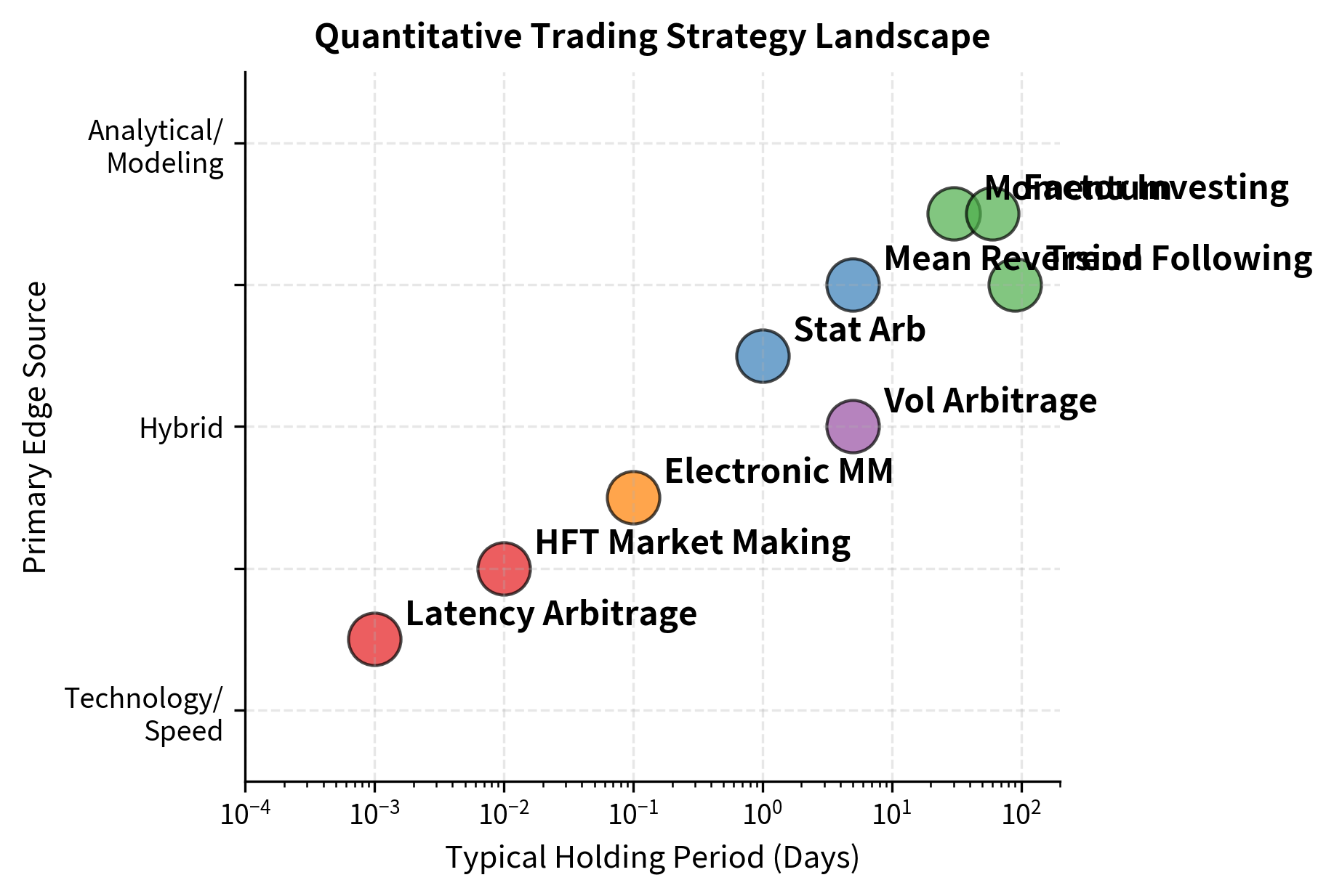
The strategy landscape reveals a fundamental tradeoff. Shorter holding periods generally require greater technological investment; longer holding periods compete primarily on analytical sophistication. Most of you find your comparative advantage falls somewhere in this spectrum.

Developing a quantitative trading strategy follows a structured process designed to maximize the probability of finding genuine alpha while minimizing the risk of overfitting to historical noise. The workflow moves through distinct phases, each with its own challenges and best practices.

Every quantitative strategy begins with an idea, a hypothesis about some market inefficiency that can be exploited. Good ideas come from multiple sources:

• Academic research: Finance and economics journals publish thousands of studies on return predictability
• Industry observation: Patterns in how institutions trade or constraints they face
• Structural analysis: Understanding market microstructure, clearing mechanisms, or regulatory impacts
• Cross-asset analogies: Applying successful ideas from one market to another

The key discipline at this stage is formulating ideas as testable hypotheses. Rather than "I think momentum works," the hypothesis should be precise: "Stocks in the top decile of 12-month past returns, excluding the most recent month, will outperform stocks in the bottom decile by at least 6% annually over the next month."

Quantitative strategies are only as good as the data underlying them. This phase involves:

• Identifying required data: Prices, fundamentals, alternative data, or proprietary datasets
• Sourcing and acquiring data: From vendors, exchanges, web scraping, or internal systems
• Cleaning and validation: Handling missing values, outliers, and data errors
• Point-in-time alignment: Ensuring you only use information available at each historical point

The last point deserves special emphasis. Financial data is frequently restated or revised. Using final, revised data in backtests introduces look-ahead bias: the model appears to use information that wasn't actually available at the time.

A small revision of 2% per quarter might seem trivial, but over many securities and time periods, using revised data systematically overstates the information advantage a strategy would have in live trading.

The signal is the quantitative measure that drives trading decisions. It translates raw data into a prediction about future returns. Signal construction involves:

• Feature engineering: Transforming raw data into predictive variables
• Normalization: Making signals comparable across assets and time periods
• Combination: Blending multiple signals into a composite indicator

A well-constructed signal should have:

• Intuitive interpretation: You should understand what high or low values mean
• Predictive content: Statistical relationship with future returns
• Diversification: The signal captures information not fully embedded in prices
• Stability: The signal doesn't change dramatically from small data perturbations

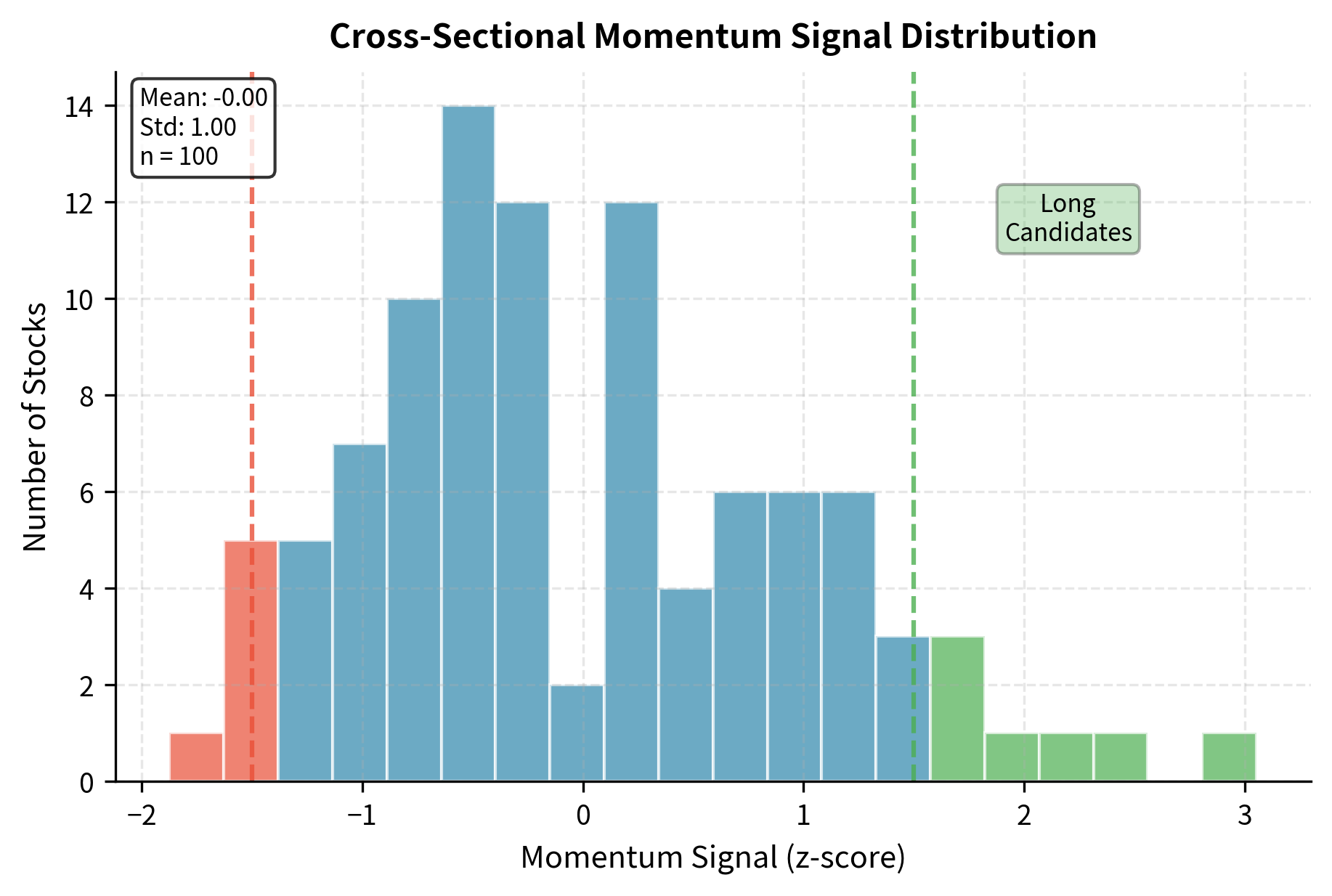
The z-score normalization ensures the signal is comparable across time periods with different market volatility, centering at zero with unit standard deviation. This standardization is essential because raw momentum values would vary dramatically depending on whether the market experienced a bull run or a crash during the lookback period. By normalizing cross-sectionally, we focus on relative momentum: which stocks have outperformed their peers, regardless of the overall market environment.

Key ParametersLink Copied

The key parameters for the momentum signal construction are:

• lookback: The window for calculating past returns (12 months). Captures the medium-term trend. Academic research has consistently found that the 12-month lookback period balances capturing persistent trends while avoiding noise.
• skip: The exclusion period (1 month). Removes the short-term reversal effect commonly found in equity markets. This exclusion is critical because stocks that performed well in the most recent month often experience mean reversion in the following month.

Backtesting applies the strategy to historical data to estimate how it would have performed. This is the most dangerous phase of strategy development because it's where overfitting most commonly occurs.

A rigorous backtesting framework must:

• Respect the arrow of time: Only use information available at each decision point
• Account for transaction costs: Include realistic estimates of spreads, commissions, and market impact
• Handle realistic execution: Assume trades occur at achievable prices, not idealized marks
• Track full portfolio dynamics: Maintain positions, cash, and margin correctly

The backtest results indicate a promising strategy with positive annualized returns and a Sharpe ratio above 1.5, suggesting good risk-adjusted performance. The turnover rate is moderate, implying that transaction costs will be manageable but must be monitored.

Key ParametersLink Copied

The key parameters for the backtest implementation are:

• top_quantile / bottom_quantile: The fraction of stocks to hold long and short (0.2). Controls portfolio concentration. Selecting 20% of stocks on each side provides diversification while maintaining sufficient differentiation between winners and losers.
• transaction_cost: The estimated cost per trade (0.001 or 10 bps). Accounts for execution friction to ensure realistic performance estimates. This includes bid-ask spread, commissions, and a small allowance for market impact.

Raw backtest results tell only part of the story. Statistical validation determines whether the results are likely to reflect genuine alpha or simply random chance. The challenge is that financial data is noisy, and even strategies with no true edge will sometimes produce impressive backtests purely by luck.

The most critical consideration is multiple testing. If we test 100 different strategy variations and select the best one, we're virtually guaranteed to find something that looks good purely by chance. This phenomenon, sometimes called data snooping or p-hacking, is one of the most insidious problems in quantitative finance.

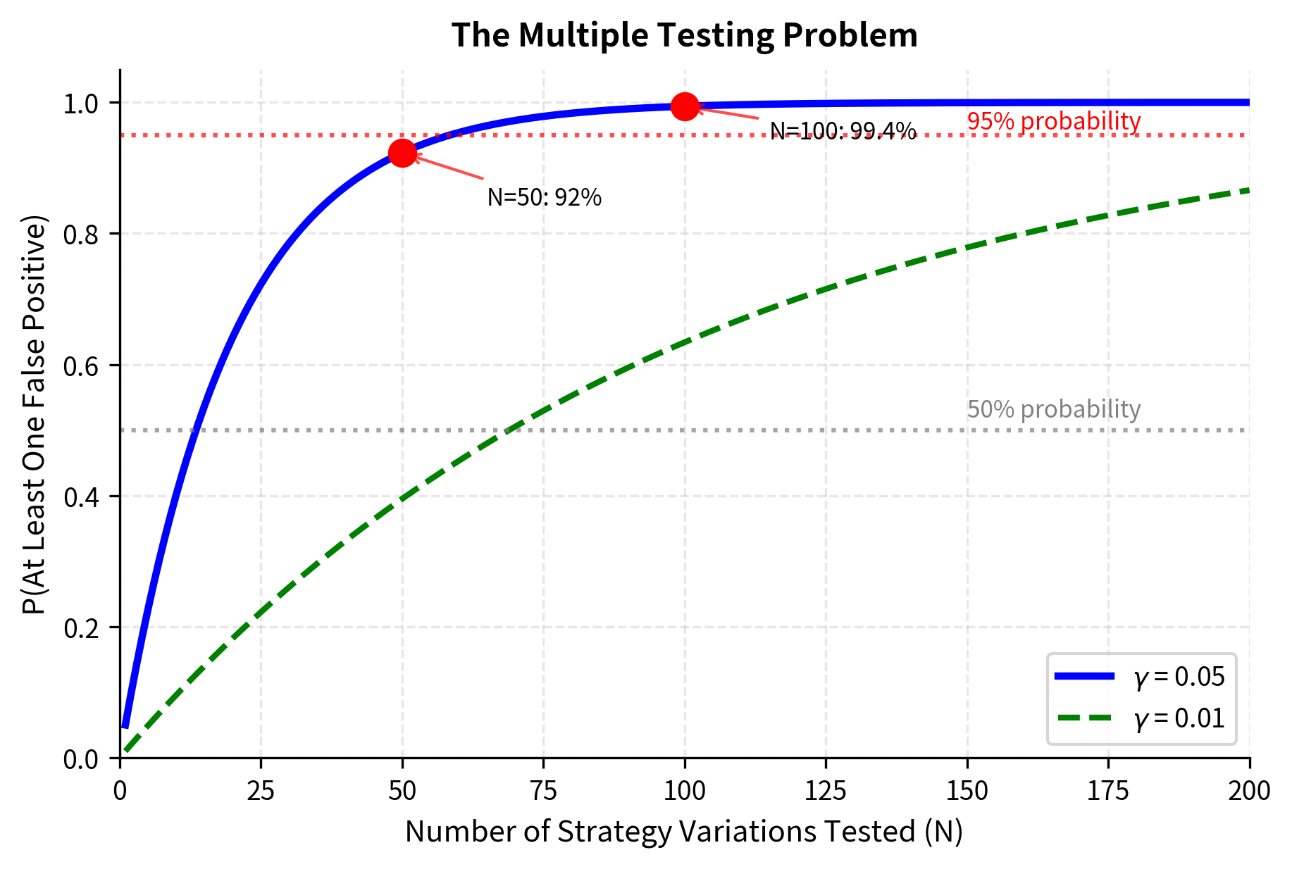
The mathematics of multiple testing reveals why this is so dangerous. The probability of finding at least one false positive increases with the number of tests. When we conduct a single statistical test at a significance level $\gamma$, we accept a $\gamma$ probability of incorrectly rejecting the null hypothesis when it is true. But when we run many tests, these individual error probabilities compound. For significance level $\gamma$ and $N$ independent tests:

To understand this formula, consider what it means for zero false positives to occur. Each individual test has a probability $(1 - \gamma)$ of correctly avoiding a false positive. For all $N$ tests to simultaneously avoid false positives, we need all $N$ of these events to happen, and since the tests are independent, we multiply these probabilities:

• $\gamma$: significance level (e.g., 0.05), the probability of a false positive in any single test
• $N$: number of strategy variations tested
• $(1 - \gamma)$: probability that a single test correctly avoids a false positive
• $(1 - \gamma)^N$: probability that all $N$ tests simultaneously avoid false positives

The formula relies on the logic of complementary probabilities: it is easier to calculate the chance that everything goes right and subtract that from 1 than to sum up all the ways something could go wrong.

For 100 tests at a 5% level, the calculation reveals a sobering truth:

This result is striking: if we test 100 strategy variations and use the standard 5% significance threshold, we are almost certain to find at least one that appears statistically significant even if none of them have any genuine predictive power.

Addressing this requires:

• Bonferroni correction: Divide the significance threshold by the number of tests
• False discovery rate control: Use methods like Benjamini-Hochberg to control the expected proportion of false discoveries
• Out-of-sample testing: Reserve a portion of data never used during development

The confidence interval provides crucial context. A Sharpe ratio of 1.5 sounds impressive, but if the confidence interval spans from -0.5 to 3.5, we have very little certainty about the true performance. The width of this interval reflects the inherent uncertainty in estimating performance from limited historical data. A narrow confidence interval that excludes zero provides much stronger evidence of genuine alpha than a point estimate alone.

Key ParametersLink Copied

The key parameters for the bootstrap test are:

• n_bootstrap: Number of resampled datasets to generate (1000). Higher values provide more precise p-value estimates. The bootstrap method works by simulating what the Sharpe ratio distribution would look like if we could repeatedly sample from the true return distribution.
• confidence_level: Probability that the true value falls within the interval (0.95). A 95% confidence level is standard, meaning we expect the true Sharpe ratio to fall within our interval 95% of the time if we repeated this analysis many times.

Before deploying capital, you must understand the strategy's risk characteristics. Building on the risk management frameworks from Part V, key questions include:

• Drawdown analysis. What are the worst historical losses, and how long did recovery take?
• Tail risk. Are returns normally distributed, or are there fat tails?
• Correlation regime. How does the strategy perform in different market conditions?
• Leverage implications. How do borrowing costs and margin requirements affect returns?

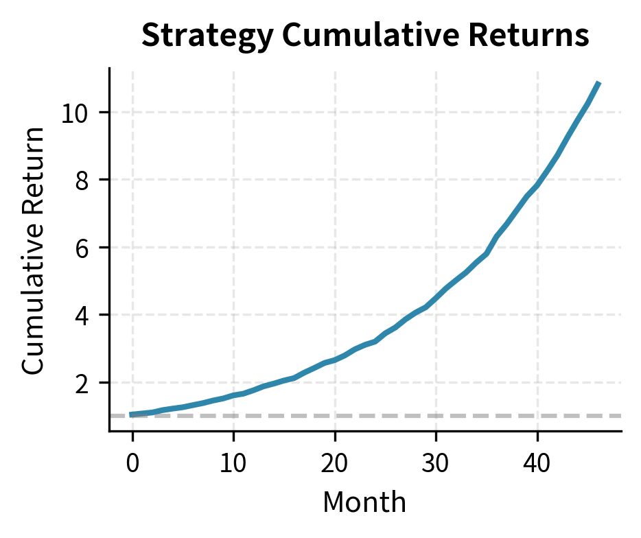
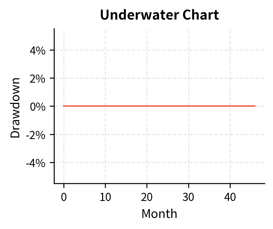
The cumulative returns chart visualizes the strategy's growth path, showing steady compounding with minor interruptions. The underwater chart complements this by highlighting the depth and duration of historical drawdowns, providing a clear view of the pain periods you would endure.

The return-to-maximum-drawdown ratio (sometimes called the Calmar ratio) indicates how much return the strategy generates per unit of maximum loss experienced. A ratio above 1.0 means annual returns exceed the worst peak-to-trough loss.

Evaluating quantitative strategies requires metrics that capture different dimensions of performance. As we covered in Part IV, Chapter 4, no single number tells the whole story. Each metric highlights a different aspect of risk and return, and together they provide a comprehensive picture of strategy quality.

The fundamental challenge in evaluating strategies is that raw returns alone are insufficient. A strategy that returns 20% annually sounds impressive until you learn it has 40% volatility, making large losses extremely likely. Risk-adjusted metrics solve this problem by normalizing returns by the risk taken to achieve them.

The Sharpe ratio remains the most widely used metric, and for good reason: it provides a universal yardstick for comparing strategies regardless of their volatility levels. The formula is elegantly simple:

Each component has a clear interpretation:

• $r_p$: portfolio return, the raw performance we observe
• $r_f$: risk-free rate, the return available from Treasury bills or similar instruments
• $E[r_p - r_f]$: expected excess return, measuring how much the strategy earns above the risk-free rate on average
• $\sigma_p$: standard deviation (volatility) of portfolio returns, measuring the typical size of fluctuations

The ratio measures the excess return generated per unit of total risk, allowing comparison between strategies with different volatility profiles. The intuition is straightforward: we care about how much extra return we earn for each unit of uncertainty we bear. An annualized Sharpe ratio above 1.0 is generally considered good, indicating the strategy earns one percentage point of excess return for each percentage point of volatility. A Sharpe above 2.0 is exceptional and rare in practice.

The Sortino ratio addresses a fundamental limitation of the Sharpe ratio. Standard deviation treats upside volatility the same as downside volatility, but you care primarily about losses. A strategy with high volatility driven entirely by large gains is actually desirable, yet the Sharpe ratio would penalize it. The Sortino ratio corrects this by penalizing only downside volatility:

where:

• $r_p$: portfolio return
• $r_f$: risk-free rate
• $\sigma_{\text{down}}$: downside deviation (calculated using only returns below a target, typically 0 or $r_f$)

This modification means the Sortino ratio rewards strategies with positively skewed returns, those that have occasional large gains but limited losses. For strategies with asymmetric return distributions, such as those that sell options or take concentrated positions, the Sortino ratio provides a more accurate assessment of risk-adjusted performance.

The Information ratio measures returns relative to a benchmark, making it essential for evaluating you when you are judged against a specific index:

where:

• $r_p$: portfolio return
• $r_b$: benchmark return
• $E[r_p - r_b]$: expected active return, the average outperformance versus the benchmark
• $\sigma_{r_p - r_b}$: tracking error (volatility of active returns), measuring how consistently the strategy beats its benchmark

This metric is central to active management, where the goal is outperforming a specific benchmark. You might have a high Sharpe ratio but a low information ratio if your returns come primarily from market exposure rather than stock selection. The information ratio isolates the value added through active decisions.

The strategy delivers consistent profitability with a high win rate and a profit factor well above 1.0. The Sortino ratio exceeds the Sharpe ratio, indicating that volatility is primarily on the upside rather than downside. This asymmetry suggests the strategy captures gains more often than it experiences losses, a desirable characteristic that the Sharpe ratio alone would not reveal.

Key ParametersLink Copied

The key parameters for performance evaluation are:

• risk_free_rate: The theoretical return of an investment with zero risk. Used as the hurdle rate for Sharpe and Sortino ratios. Typically set to the yield on short-term Treasury bills.
• benchmark_returns: Optional series of returns for a market index. Required to calculate the Information Ratio and Tracking Error. The choice of benchmark matters enormously and should reflect the strategy's investment universe.

Individual metrics can be misleading. A strategy might have a high Sharpe ratio but unacceptable maximum drawdown, or excellent returns that come with extreme tail risk. The most robust evaluation considers multiple dimensions simultaneously.

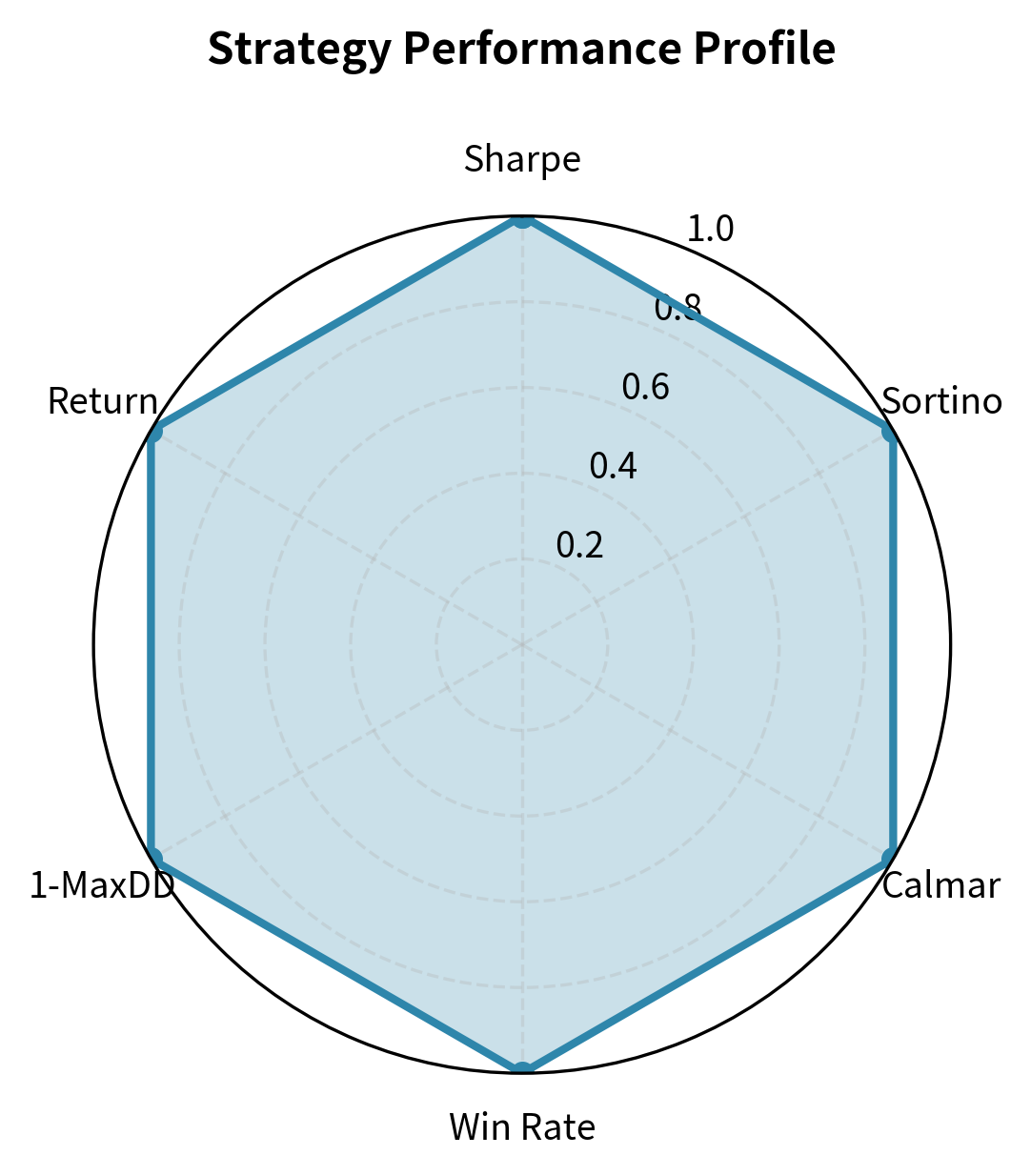
The radar chart reveals performance trade-offs at a glance. This strategy shows balanced performance across metrics, without extreme strengths or weaknesses.

The gap between backtested and live trading performance is one of the most frustrating aspects of quantitative finance. Strategies that look phenomenal in historical testing often fail in production. Understanding the common pitfalls helps avoid them.

Look-ahead bias occurs when the backtest uses information that wasn't available at the time. Examples include:

• Using end-of-day prices for decisions made during trading hours
• Using revised financial data instead of originally reported values
• Assuming instant knowledge of index reconstitutions or corporate actions

This bias is insidious because it's often unintentional. Data vendors typically provide "as-is" data reflecting current knowledge, not point-in-time data showing what was known historically.

Survivorship bias results from testing only on securities that survived to the present, ignoring those that delisted, went bankrupt, or were acquired. This systematically overestimates returns because the worst performers are excluded.

Consider a value strategy that buys cheap stocks. Many cheap stocks are cheap because they're headed toward bankruptcy. A survivorship-biased backtest never sees these losses because those companies aren't in the database.

Overfitting occurs when a model captures noise in the training data rather than genuine signal. The model performs well historically but fails on new data.

Signs of overfitting include:

• Strategy requires many parameters or complex rules
• Performance is sensitive to small parameter changes
• Out-of-sample performance degrades significantly
• Strategy works only on specific subperiods

The antidote is simplicity, economic rationale, and rigorous out-of-sample testing. As a rule of thumb, simpler strategies with clear economic logic are more likely to survive in live trading.

Backtests often assume unrealistically low transaction costs. Real-world trading involves:

• Bid-ask spreads: The immediate cost of crossing the spread
• Market impact: Moving prices against you when trading large positions
• Slippage: Execution prices worse than expected due to latency
• Borrowing costs: Fees for shorting stocks, which can be substantial for hard-to-borrow names

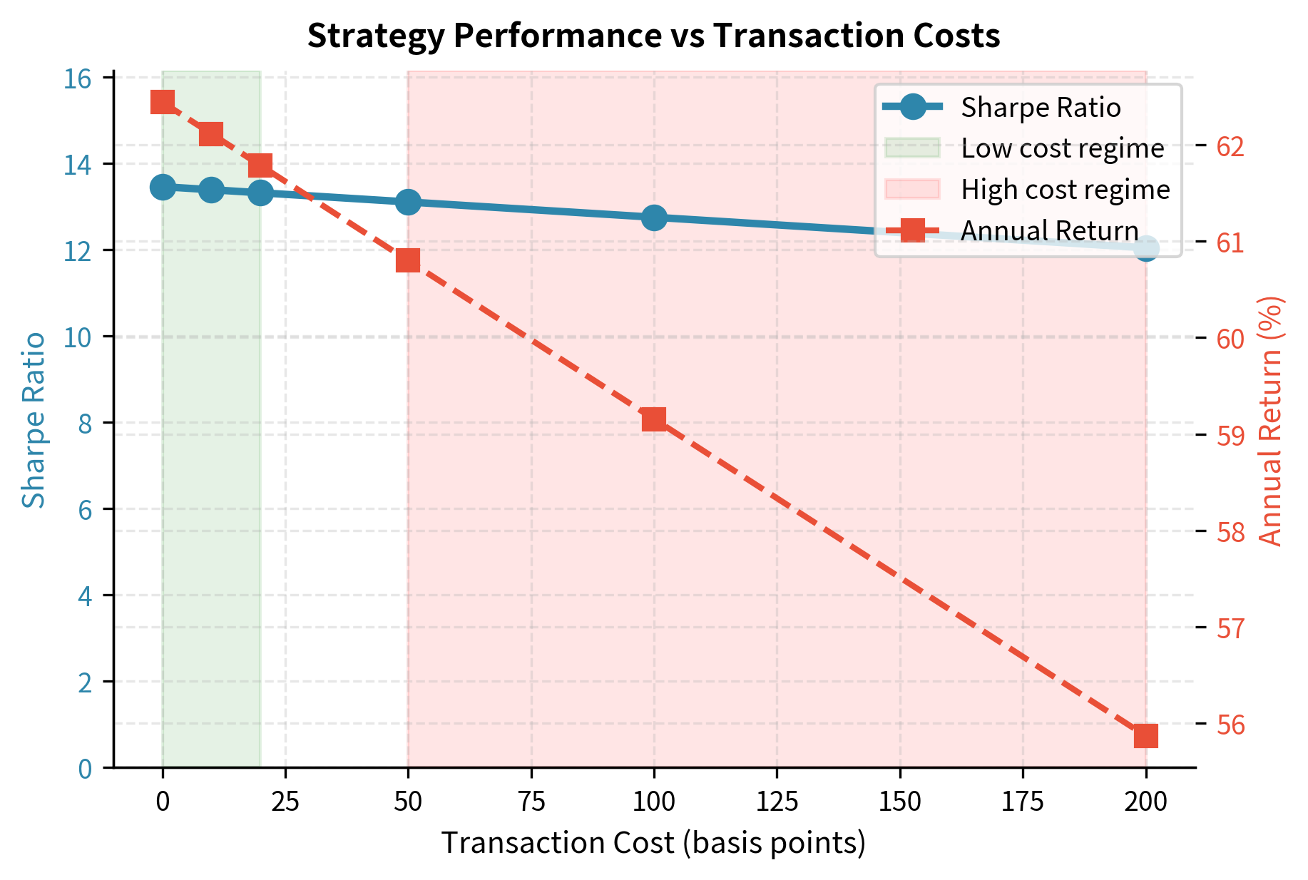
The table reveals how sensitive the strategy is to transaction cost assumptions. A strategy that looks profitable at 10 basis points per trade might be worthless at 50 basis points. High-turnover strategies are particularly vulnerable.

Key ParametersLink Copied

The key parameters for sensitivity analysis are:

• cost_levels: Range of transaction cost assumptions (0 to 20 bps). Tests strategy robustness against execution friction.
• turnover: The portfolio turnover rate. Determines how heavily transaction costs impact net returns.

The transition from backtest to live trading represents the ultimate test of a quantitative strategy. Several additional considerations arise:

Before risking real capital, run the strategy in a paper trading environment. This stage validates:

• Execution infrastructure works correctly
• Data feeds are reliable and timely
• Order management handles edge cases
• Risk controls trigger appropriately

Paper trading also provides a psychological bridge, allowing you to experience the strategy's behavior in real-time without financial consequence.

Even a profitable strategy can blow up if position sizes are too large. Building on the risk management principles from Part V, key decisions include:

• Capital allocation. How much of total capital to deploy
• Position limits. Maximum size for individual positions
• Sector and factor limits. Concentration limits to ensure diversification
• Drawdown triggers. Conditions for reducing or halting the strategy

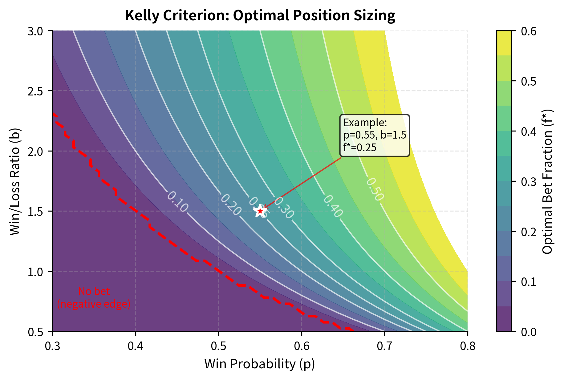
The Kelly criterion provides theoretical guidance on optimal bet sizing. The fundamental question Kelly addresses is: given a trading opportunity with known probabilities of winning and losing, what fraction of your capital should you risk to maximize long-term wealth growth? Betting too little leaves money on the table, while betting too much risks catastrophic losses.

The formula can be derived by maximizing the expected logarithm of wealth, which naturally balances return against risk:

Each variable captures a key aspect of the trading opportunity:

• $f^*$: optimal fraction of capital to allocate, the output we seek
• $p$: probability of a winning trade, estimated from historical analysis
• $q$: probability of a losing trade ($1 - p$), the complement of the win probability
• $b$: win/loss ratio (average gain divided by average loss), measuring the payoff structure
• $bp - q$: expected net profit of the trade (the edge), combining probability and magnitude

The formula balances the strategy's edge against the risk of variance:

• The numerator represents the edge: the expected return per unit of risk. A positive edge means the strategy is profitable on average. The larger the edge, the more capital we should allocate.
• The denominator represents the odds: scaling the bet size inversely to the payoff ratio. When wins are much larger than losses (high $b$), we can afford smaller position sizes because each win contributes more. When the win/loss ratio is closer to 1, we need larger positions to capitalize on our edge.

By maximizing the expected logarithm of wealth, this formula determines the position size that yields the highest long-term geometric growth rate, explicitly penalizing volatility to avoid the ruin associated with over-betting. The logarithmic objective is crucial: it naturally incorporates risk aversion because the pain of losing half your wealth outweighs the joy of doubling it.

In practice, most of us use fractional Kelly (e.g., half Kelly) to account for estimation uncertainty. The probabilities and payoff ratios used in the Kelly formula are estimates, and overconfidence in these estimates leads to position sizes that are too large. Using half or quarter Kelly provides a margin of safety against parameter estimation errors.

Live strategies require continuous monitoring. Key metrics to track include:

• Performance versus expectation: Is the strategy performing within backtested parameters?
• Factor exposures: Have risk exposures drifted from intended levels?
• Execution quality: Are fills occurring at expected prices?
• Capacity utilization: Is the strategy experiencing increasing market impact?

Strategies also decay over time as the market learns and adapts. You continuously research new signals and retire strategies that have stopped working.

This chapter established the conceptual foundation for quantitative trading strategies. The key takeaways are:

• Alpha represents genuine skill, measured as returns unexplained by exposure to systematic risk factors. The search for alpha is the central challenge of quantitative finance, requiring both analytical rigor and economic intuition.

• Strategy categories span a wide spectrum from high-frequency market making to long-horizon factor investing. Each category has distinct characteristics in terms of holding periods, required infrastructure, and the nature of the competitive edge exploited.

• The development workflow is structured and disciplined: idea generation, data preparation, signal construction, backtesting, statistical validation, and risk assessment. Each phase has specific best practices designed to maximize the probability of finding genuine alpha.

• Rigorous backtesting is essential but dangerous. The same flexibility that allows comprehensive testing also enables overfitting. Success requires simplicity, economic rationale, out-of-sample validation, and realistic assumptions about transaction costs and execution.

• Performance evaluation requires multiple metrics. Sharpe ratio, Sortino ratio, maximum drawdown, and information ratio each capture different aspects of performance. The best strategies show strong, balanced performance across multiple dimensions.

• The transition to live trading introduces new challenges. Paper trading, position sizing, risk limits, and ongoing monitoring are essential for translating backtested results into real profits.

In the following chapters, we'll dive deep into specific strategy categories. We'll explore mean reversion and statistical arbitrage, where profit comes from betting on relationships returning to normal. We'll examine trend following and momentum, strategies that profit from the persistence of price moves. We'll cover factor investing with its systematic approach to capturing risk premia, and we'll investigate the specialized world of volatility trading. Each strategy type builds on the foundational concepts introduced here while requiring its own analytical toolkit and operational considerations.

Ready to test your understanding? Take this quick quiz to reinforce what you've learned about quantitative trading strategies.