

Learn how to build long-short factor portfolios using quintile rankings. Covers value, momentum, quality, and volatility factors with exposure analysis.
Choose your expertise level to adjust how many terms are explained. Beginners see more tooltips, experts see fewer to maintain reading flow. Hover over underlined terms for instant definitions.
Factor Investing and Long/Short Equity
Factor investing represents one of the most significant developments in quantitative finance over the past half-century. At its core, factor investing is the systematic pursuit of risk premia, which are the excess returns associated with exposure to specific characteristics or "factors" that explain cross-sectional differences in stock returns. Rather than viewing a portfolio as simply a collection of individual stocks, factor investing decomposes returns into exposures to fundamental drivers like value, size, momentum, and quality. This perspective shift transforms how we think about portfolio construction: instead of picking stocks, we are harvesting systematic sources of return that have persisted across decades and geographies.
The intellectual foundation for factor investing emerged from the Capital Asset Pricing Model and Arbitrage Pricing Theory, which we explored in Part IV. While CAPM proposed that market beta alone explains expected returns, decades of empirical research revealed persistent anomalies: patterns of returns that CAPM could not explain. These anomalies became the building blocks of factor investing: small stocks outperforming large stocks, cheap stocks beating expensive ones, and recent winners continuing to outperform recent losers. What began as academic curiosities became the foundation of a multi-trillion dollar industry.
Long/short equity strategies operationalize these insights by simultaneously buying stocks with favorable factor characteristics and selling short those with unfavorable characteristics. This approach allows investors to isolate factor returns from overall market movements, potentially generating alpha regardless of whether the market rises or falls. The result is a powerful toolkit that forms the backbone of quantitative hedge funds managing trillions of dollars globally. By going both long and short, investors can neutralize their exposure to broad market movements and focus purely on capturing the spread between stocks with desirable and undesirable characteristics.
This chapter bridges the theoretical factor models we studied earlier with practical portfolio construction. You will learn how to define, measure, and combine factors into systematic strategies, understand the mechanics of long/short portfolio construction, and appreciate the risk management challenges that arise when factors temporarily underperform. By the end, you will have a complete framework for building and analyzing factor-based investment strategies.
The Factor Zoo: Canonical Factors and Their Rationale
Academic research has documented hundreds of variables that predict stock returns, leading researchers to describe a "factor zoo" of potential alpha sources. This proliferation raises important questions: Which factors are real, and which are artifacts of data mining? However, a handful of factors have proven robust across markets, time periods, and academic scrutiny. These canonical factors form the foundation of most systematic equity strategies and have withstood rigorous out-of-sample testing across different countries and time periods.
Value
The value factor captures the tendency of cheap stocks, those trading at low prices relative to fundamentals, to outperform expensive stocks over time. This phenomenon has been observed for nearly a century and remains one of the most studied relationships in finance. Fama and French's seminal 1992 paper documented that stocks with high book-to-market ratios earned higher average returns than stocks with low book-to-market ratios, even after controlling for market risk. This finding challenged the efficient market hypothesis and sparked intense debate about whether the premium represents compensation for risk or evidence of systematic investor mispricing.
The value factor represents the return spread between stocks trading at low prices relative to fundamental value and stocks trading at high prices relative to fundamental value. Common value metrics include price-to-book, price-to-earnings, price-to-cash-flow, and enterprise value-to-EBITDA. The core intuition is that buying assets for less than their intrinsic worth should, on average, generate superior returns.
The rationale for the value premium remains debated, and understanding these competing explanations helps investors appreciate when the premium might be stronger or weaker. Risk-based explanations suggest that cheap stocks are genuinely riskier: they may be distressed companies facing financial difficulty, and investors demand compensation for bearing this risk. Under this view, the value premium is fair compensation for holding stocks that perform poorly during economic downturns when investors most need their wealth. Behavioral explanations propose that investors systematically overreact to bad news, pushing prices below fundamental value, or that they extrapolate recent poor performance too far into the future. This perspective suggests the premium exists because human psychology creates predictable mispricings that patient investors can exploit.
The key value metrics used in practice include:
- Book-to-Price (B/P): Book value of equity divided by market capitalization. Higher values indicate cheaper stocks relative to their accounting value. This metric works best for capital-intensive industries where book value meaningfully reflects economic worth.
- Earnings-to-Price (E/P): Earnings per share divided by stock price, the inverse of the P/E ratio. This captures cheapness relative to current profitability and is widely followed by fundamental investors.
- Cash Flow-to-Price (CF/P): Operating cash flow divided by market capitalization, useful for capital-intensive industries where depreciation choices can distort earnings. Cash flow metrics are harder for management to manipulate than accounting earnings.
- EBITDA-to-Enterprise Value: Operating earnings before interest, taxes, depreciation, and amortization divided by total enterprise value, allowing comparison across capital structures. This metric is particularly useful when comparing companies with different levels of debt.
Size
The size factor reflects the historical tendency of small-capitalization stocks to outperform large-capitalization stocks. This "small firm effect" was documented by Rolf Banz in 1981 and later incorporated into the Fama-French three-factor model. The size premium was one of the earliest documented anomalies and sparked the empirical finance revolution that continues today.
Small stocks may earn higher returns because they are genuinely riskier: they have less diversified revenue streams, fewer resources to weather economic downturns, and lower liquidity. These characteristics make small-cap stocks more sensitive to economic conditions and more costly to trade in large quantities. Alternatively, small stocks may be overlooked by institutional investors and analysts, creating pricing inefficiencies that can be exploited by investors willing to do the research. With fewer eyes scrutinizing these companies, mispricings may persist longer than in large-cap stocks where every piece of information is rapidly incorporated into prices.
The size factor, often called SMB (Small Minus Big), represents the return spread between small-capitalization stocks and large-capitalization stocks. It is typically measured using market capitalization, with small stocks in the bottom tercile or quintile of the market. The factor captures the idea that smaller companies, though riskier and less liquid, offer compensation for these drawbacks through higher expected returns.
Momentum
As we explored in the previous chapter on trend following, momentum captures the tendency of recent winners to continue outperforming and recent losers to continue underperforming. Cross-sectional momentum ranks stocks by their past returns (typically over the prior 12 months, excluding the most recent month to avoid short-term reversal effects) and goes long winners while shorting losers. The exclusion of the most recent month is crucial because very short-term returns exhibit reversal rather than continuation.
The momentum premium is one of the most robust anomalies in finance, observed across virtually all asset classes and geographic markets. Its universality is striking: momentum works in stocks, bonds, currencies, and commodities, and has been documented in markets from the United States to Japan to emerging economies. Behavioral explanations center on investor underreaction to information and subsequent trend-chasing behavior. When good news arrives, investors initially underreact, causing prices to adjust slowly. As more investors recognize the positive trend, they pile in, pushing prices further in the same direction. Risk-based explanations have proven more elusive, making momentum particularly challenging for efficient market theorists who believe that predictable patterns should be quickly arbitraged away.
Quality
The quality factor captures the outperformance of high-quality companies (those with strong profitability, stable earnings, low leverage, and conservative accounting) relative to low-quality companies. Quality emerged more recently as a distinct factor but has become a cornerstone of modern factor investing. The intuition is compelling: well-run companies with sustainable competitive advantages should outperform poorly-run companies with unstable earnings and excessive debt.
The quality factor represents the return spread between high-quality firms (characterized by profitability, earnings stability, low leverage, and conservative accounting) and low-quality firms. It is sometimes decomposed into profitability and investment sub-factors. Quality reflects the idea that superior business fundamentals translate into superior stock returns, particularly when those fundamentals are not fully reflected in current prices.
Key quality metrics include:
- Return on Equity (ROE): Net income divided by shareholders' equity, measuring profitability relative to invested capital. High ROE indicates a company generates substantial profits from each dollar of shareholder investment.
- Return on Assets (ROA): Net income divided by total assets, measuring operational efficiency independent of capital structure. This metric is useful for comparing companies with different leverage levels.
- Gross Profitability: Gross profit divided by assets, a metric Novy-Marx showed to be particularly predictive of returns. This measure focuses on the core profitability of a business before overhead and financing costs obscure the picture.
- Accruals: The difference between earnings and cash flow, with low accruals indicating higher earnings quality. Companies with earnings backed by actual cash flows are less likely to experience negative earnings surprises than those with high accruals.
- Leverage: Debt-to-equity or debt-to-assets ratios, with lower leverage indicating financial strength. Companies with modest debt have more flexibility during downturns and lower risk of financial distress.
Low Volatility
The low volatility anomaly represents perhaps the most puzzling factor: stocks with lower historical volatility have historically outperformed stocks with higher volatility, contradicting the basic risk-return tradeoff taught in introductory finance. Basic financial theory suggests that investors demand higher returns for bearing more risk, yet empirically the opposite appears true. High-volatility stocks have delivered disappointing risk-adjusted returns while boring, low-volatility stocks have quietly compounded wealth.
Several explanations have been proposed for this counterintuitive finding. Institutional investors may be constrained from using leverage, leading them to chase high-beta stocks to amplify returns, which bids up prices and reduces expected returns. If pension funds and mutual funds cannot lever up low-volatility portfolios to achieve their return targets, they instead buy high-volatility stocks, pushing prices above fair value. Lottery preferences may cause retail investors to overpay for volatile stocks with large potential payoffs. The appeal of potentially "hitting it big" leads investors to bid up speculative stocks, similar to how lottery tickets are overpriced relative to their expected value. Benchmarking behavior may discourage active managers from holding low-volatility stocks that deviate significantly from index weights, reducing demand for these securities and keeping prices attractively low.
The low volatility factor is typically constructed using realized volatility over the past one to three years, or using beta relative to the market. Both approaches capture similar stocks, though they represent conceptually different risks. Volatility measures a stock's overall variability, while beta specifically captures sensitivity to market movements.
Growth
Growth investing focuses on companies with strong earnings growth, revenue expansion, and improving fundamentals. While growth is sometimes viewed as the opposite of value (since high-growth stocks often trade at premium valuations), it represents a distinct factor capturing investor appetite for companies with expanding business prospects. The tension between value and growth represents one of the oldest debates in investing, with practitioners often falling into one camp or the other.
Growth metrics include:
- Earnings Growth: Historical or expected growth in earnings per share. Companies that consistently grow earnings tend to see share price appreciation, though much depends on whether growth meets or exceeds expectations.
- Revenue Growth: Historical or expected growth in sales. Top-line growth indicates expanding market opportunity, though profitability matters for translating revenue growth into shareholder value.
- Asset Growth: Change in total assets, though this metric has a negative relationship with future returns (high asset growth firms tend to underperform). This counterintuitive finding suggests that aggressive expansion often destroys value, perhaps because managers pursue growth for its own sake rather than shareholder returns.
Constructing Factor Portfolios
Building a factor portfolio requires translating abstract factor definitions into concrete portfolio weights. The standard approach involves ranking stocks by factor characteristics, forming portfolios based on these rankings, and establishing long positions in stocks with favorable characteristics while shorting those with unfavorable characteristics. This process transforms academic insights into implementable investment strategies.
Factor Scoring and Ranking
The first step in factor portfolio construction is computing factor scores for each stock in the investment universe. For a single factor like value, this might involve calculating book-to-price ratios for all stocks. For multi-factor strategies, you must combine scores across multiple characteristics. The challenge lies in creating scores that are comparable across different metrics and meaningful in terms of predicting future returns.
Factor scores are typically standardized to ensure comparability across different metrics. Without standardization, factors measured in different units or with different scales cannot be meaningfully combined. A book-to-price ratio might range from 0.1 to 3.0, while momentum returns might range from -50% to +100%. Z-score normalization transforms each factor to have zero mean and unit standard deviation within each cross-section, placing all factors on a common footing:
The normalized scores now share a common scale, making it straightforward to combine them or compare stocks across different factors. A stock with a value z-score of +2.0 is two standard deviations cheaper than average, directly comparable to a momentum z-score of +2.0 indicating a stock that has outperformed by two standard deviations. This standardization is essential for building multi-factor strategies where we want to weight different characteristics according to their importance.
Quintile Portfolio Formation
A standard approach for isolating factor returns involves sorting stocks into quintile portfolios based on factor scores. This methodology, pioneered by Fama and French, has become the industry standard for testing factor hypotheses and constructing factor portfolios. Stocks in the top quintile (Q5) receive long positions, while stocks in the bottom quintile (Q1) receive short positions. The middle quintiles (Q2-Q4) are excluded, maximizing the spread between factor exposures. By focusing on the extremes, we capture the full range of the factor premium while avoiding stocks with ambiguous factor characteristics.
The long/short portfolio holds the top quintile (highest book-to-price, cheapest stocks) long and the bottom quintile (lowest book-to-price, most expensive stocks) short. The expected return of this portfolio isolates the value premium from overall market movements. If value stocks on average earn 2% more per year than growth stocks, this premium shows up in the long/short portfolio return regardless of whether the overall market is up or down. This isolation makes factor returns a cleaner signal for understanding what drives equity returns.
Weighting Schemes
Within each quintile, stocks can be weighted using several approaches, each with distinct advantages and drawbacks:
-
Equal weighting: Each stock receives identical weight, maximizing diversification within the quintile. This approach gives significant weight to small-cap stocks, which may introduce unintended size exposure and liquidity challenges. However, equal weighting treats each stock as an independent bet on the factor, which may be appropriate if we believe factor characteristics predict returns equally well for all stocks.
-
Market-cap weighting: Stocks are weighted by market capitalization, giving larger companies more influence. This reduces transaction costs and improves liquidity but may dilute factor exposure since large-cap stocks often have weaker factor characteristics. Market-cap weighting reflects the economic reality that large companies represent more investable opportunities, but it also means the portfolio is dominated by a few large names.
-
Factor-score weighting: Stocks are weighted proportionally to their factor scores, tilting more heavily toward stocks with stronger characteristics. This maximizes factor exposure but concentrates the portfolio in fewer names. If we believe that the cheapest stocks will outperform moderately cheap stocks, score weighting makes sense. However, it introduces concentration risk and may reduce diversification benefits.
The equal-weighted portfolio has a net exposure of approximately zero (long weights sum to +1, short weights sum to -1), making it market-neutral at inception. This isolation of factor returns from market beta is a key feature of long/short factor portfolios. The portfolio's performance depends only on whether cheap stocks outperform expensive stocks, not on whether the overall market rises or falls. This property makes factor investing particularly valuable for investors seeking uncorrelated returns or those who want to express factor views without making market timing bets.
Sector Neutralization and Risk Control
Raw factor portfolios often carry unintended sector exposures that can dominate returns and obscure the underlying factor performance. Value stocks, for example, tend to cluster in sectors like financials and energy, while growth stocks dominate technology and healthcare. These sector tilts can dominate factor returns and introduce risks unrelated to the factor itself. Without careful control, a "value" portfolio might actually be a bet on energy prices or banking regulation.
Why Sector Neutrality Matters
Consider a value portfolio constructed without sector constraints. During a period when energy stocks decline sharply due to falling oil prices, the value portfolio may underperform even if value stocks outperform within each sector. The sector exposure masks the true factor performance. An investor who thought they were capturing the value premium discovers they were actually making a concentrated bet on oil prices. This conflation of factor and sector returns makes it difficult to evaluate strategy performance and manage risk.
Sector neutralization constructs portfolios that have zero net exposure to each sector. The long leg's sector weights match the short leg's sector weights, ensuring that sector movements cancel out and only the pure factor return remains. If the long portfolio holds 10% in technology stocks, the short portfolio also holds 10% in technology stocks (but shorting the most expensive ones). Any sector-wide movements affect both legs equally, leaving only the within-sector selection to drive returns.
The sector-neutral portfolio has near-zero net exposure within each sector, meaning sector returns do not affect portfolio performance. Any remaining small imbalances result from rounding in the quintile assignments and can be further refined with optimization. This construction ensures that when we measure portfolio performance, we are truly capturing the value premium rather than sector rotation effects disguised as factor returns.
Beta Neutralization
Beyond sector neutrality, many long/short strategies target beta neutrality: zero correlation with the overall market. This is achieved by adjusting position sizes so that the weighted average beta of long positions equals the weighted average beta of short positions. The goal is to construct a portfolio whose expected return is independent of whether the market goes up or down.
As we discussed in Part IV on CAPM, a stock's beta measures its sensitivity to market movements. A stock with a beta of 1.5 is expected to move 1.5% for every 1% market move, while a stock with beta of 0.5 moves only half as much as the market. A beta-neutral portfolio has no expected return from market exposure, generating returns only from security selection and factor exposure. This property is valuable for investors seeking absolute returns uncorrelated with equity markets.
The beta-neutral portfolio scales the short leg so that its weighted beta contribution exactly offsets the long leg. This ensures the portfolio has no expected return from market movements. Note that the short scaling factor may differ from 1.0, meaning the portfolio is not necessarily dollar-neutral (equal dollar amounts long and short). The portfolio might be 105% long and 95% short, or vice versa, depending on the relative betas of value and growth stocks. The key property is that market movements have no expected impact on portfolio returns, leaving only factor-related returns.
Multi-Factor Portfolio Construction
Most sophisticated quantitative strategies combine multiple factors rather than relying on a single characteristic. Multi-factor portfolios offer several advantages that make them superior to single-factor approaches for most investors:
- Diversification: Factors have low correlations with each other, so combining them reduces portfolio volatility. When value underperforms, momentum might be doing well, and vice versa. This diversification benefit is similar to holding stocks in different industries.
- Smoother returns: Different factors outperform in different market environments, creating more consistent performance. Value tends to do well during economic recoveries, while quality performs better during market stress. Combining factors smooths the return stream.
- Higher Sharpe ratios: The risk reduction from factor diversification typically exceeds any reduction in expected returns. If each factor earns a premium, combining them captures multiple premia while benefiting from diversification. The result is higher risk-adjusted returns.
Combining Factor Scores
The most straightforward approach to multi-factor investing combines individual factor scores into a composite score. Each stock receives a score reflecting its standing across all factors, and portfolios are formed based on this composite. A stock might be moderately cheap, strongly momentum-positive, and highly profitable. The composite score aggregates these characteristics into a single ranking that can be used for portfolio construction.
The composite quintile portfolios show the expected pattern: Q5 (the long portfolio) has positive scores across all factors, while Q1 (the short portfolio) has negative scores. The composite approach captures multiple sources of alpha simultaneously. Stocks in the top quintile are cheap, have strong momentum, high profitability, and low volatility. These stocks benefit from multiple tailwinds, increasing the probability that at least some factor premia will be realized.
Factor Weight Optimization
Rather than using equal or heuristic weights, factor weights can be optimized to maximize the Sharpe ratio of the combined portfolio. This requires historical factor return estimates and covariance matrices, as we covered in Part IV on portfolio optimization. The goal is to find the combination of factor weights that maximizes risk-adjusted returns given the expected returns and correlations of each factor.
The optimization problem seeks to maximize the portfolio's Sharpe ratio, assuming a risk-free rate of zero for long/short portfolios since these strategies are self-financing:
where:
- : vector of factor weights representing the allocation to each factor
- : vector of expected factor excess returns capturing what we expect each factor to earn
- : factor return covariance matrix describing both factor volatilities and their correlations
- : expected portfolio return, the weighted average of factor returns
- : portfolio volatility, accounting for diversification benefits from low factor correlations
To derive the optimal weights, we observe that the Sharpe ratio is scale-invariant, meaning that doubling all weights does not change the ratio. We can therefore fix the expected return to a constant level (e.g., ) and minimize the portfolio variance. This transformation converts the ratio optimization into a standard quadratic programming problem. The Lagrangian for this constrained optimization is:
where:
- : Lagrangian function to be minimized, combining the objective with the constraint
- : vector of factor weights we are solving for
- : factor return covariance matrix encoding risk relationships
- : Lagrange multiplier enforcing the return constraint, representing the shadow price of the return target
- : vector of expected factor excess returns
The first term represents the portfolio variance (to be minimized), while the second term captures the constraint that the expected return must equal 1. This formulation follows the standard approach in constrained optimization where we convert an inequality or equality constraint into part of the objective function.
Taking the derivative with respect to and setting it to zero yields the first-order optimality condition:
Since is just a scalar scaling factor that does not affect relative weights, the relative weights are determined solely by the product of the inverse covariance matrix and the expected returns:
where:
- : optimal factor weights that maximize the Sharpe ratio
- : inverse of the covariance matrix (also called the precision matrix), encoding information about factor volatilities and correlations
- : expected factor excess returns
This elegant formula has a clear intuition. The precision matrix automatically accounts for correlations between factors. It assigns higher weights to factors with high returns and low volatility, while penalizing factors that are highly correlated with others to maximize diversification benefits. A factor with high expected returns but also high correlation with other factors receives less weight than a factor with moderate returns but unique diversification properties.
The optimization tilts heavily toward factors with favorable risk-return characteristics. In this example, Quality receives a large weight due to its high Sharpe ratio (modest returns but low volatility), while Momentum, despite having the highest expected return, receives less weight due to its higher volatility and negative correlation with Value. The negative correlation between Value and Momentum is actually valuable for diversification, but the optimization accounts for this automatically through the covariance matrix inversion. The result is a portfolio that achieves a higher Sharpe ratio than simple equal weighting.
Long/Short Equity Hedge Funds
Long/short equity hedge funds apply factor investing principles within an active management framework. Unlike systematic factor portfolios that mechanically follow rules, hedge funds combine quantitative signals with discretionary judgment, sector expertise, and active risk management. This blend of art and science has made long/short equity one of the largest and most enduring hedge fund strategies.
Hedge Fund Portfolio Structure
A typical long/short equity hedge fund maintains several key portfolio characteristics that define its risk profile and return expectations:
- Gross exposure: The sum of absolute long and short positions, typically 150-200% of capital. Higher gross exposure amplifies both returns and risks. A fund with 100% long and 50% short has 150% gross exposure, meaning it has borrowed to amplify its bets.
- Net exposure: The difference between long and short positions, reflecting directional market bias. Market-neutral funds target 0% net exposure, while directional funds may maintain 20-50% net long. Net exposure determines how much the portfolio moves with the overall market.
- Position concentration: Individual position sizes, typically 2-5% for core holdings and smaller for satellite positions. Position limits ensure no single stock can devastate the portfolio.
The constructed portfolio meets the target specifications: approximately 160% gross exposure (indicating significant leverage) and 20% net long exposure (maintaining a directional bias toward the market). The portfolio holds 50 positions on each side, with position sizes controlled to prevent concentration risk. This structure allows the fund to express both factor views and a modest directional opinion while maintaining diversification.
Alpha Generation Process
Long/short hedge funds generate alpha through several mechanisms that work together to create returns:
- Factor exposure: Systematic exposure to rewarded factors provides a baseline return. The fund captures value, momentum, and quality premia through its stock selection.
- Stock selection: Within-factor selection, choosing the best value stocks rather than just any value stocks, adds additional alpha. A skilled analyst might identify which cheap stocks are genuinely undervalued versus which are value traps.
- Timing: Adjusting factor exposures based on market conditions or factor valuations can enhance returns, though this is notoriously difficult to execute consistently.
- Shorting: Identifying overvalued securities and positioning for their decline, which is unavailable to long-only investors. Shorts can generate returns when expensive stocks fall, regardless of market direction.
The ability to short is particularly valuable and represents a key advantage of hedge funds over long-only managers. Long-only managers can only underweight expensive stocks relative to a benchmark, but short sellers can directly profit from overvaluation. This asymmetry makes shorting a significant source of potential alpha, though it also introduces unique risks including short squeezes and unlimited loss potential. When a heavily shorted stock rises sharply, short sellers must buy shares to cover, pushing prices higher and potentially causing cascading losses.
Risk Management in Factor Portfolios
Factor investing introduces specific risks that require careful management beyond traditional portfolio risk measures. Factors can experience extended periods of underperformance, correlations between factors can shift, and crowded trades can amplify losses during factor rotations. Understanding these risks is essential for successfully implementing factor strategies.
Factor Drawdowns and Regime Changes
Factors experience significant drawdowns that test investor patience and conviction. The value factor, for example, underperformed growth dramatically from 2017-2020, leading some investors to question whether the value premium had disappeared. This was the longest and deepest drawdown for value in recorded history. Momentum crashed spectacularly during the March 2009 market reversal, losing years of accumulated gains in weeks as the market violently snapped back from its lows.
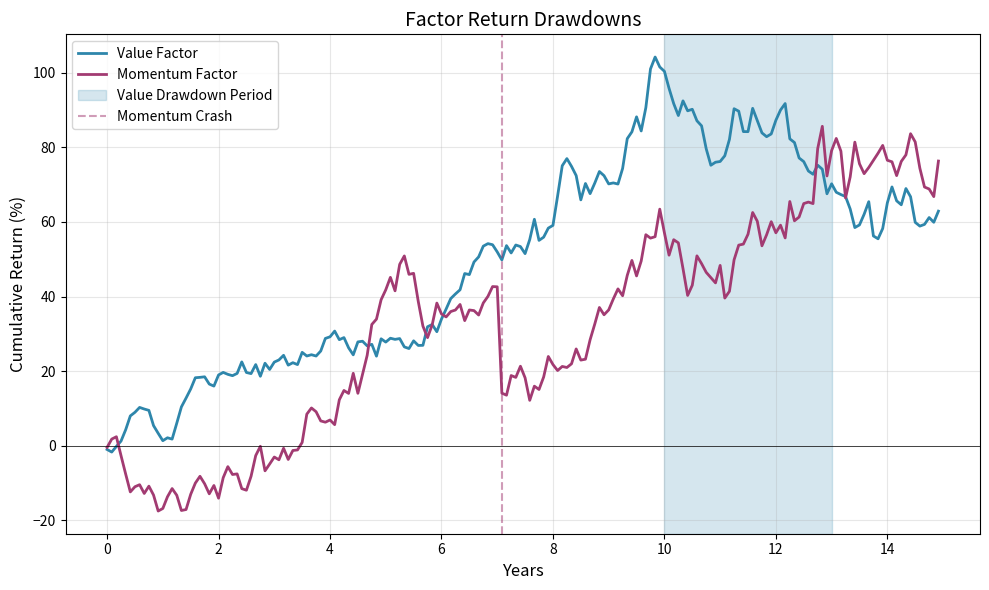
The visualization illustrates a common pattern in factor investing: extended drawdowns that test investor conviction. The value factor's three-year underperformance period could lead to redemptions, forced liquidations, and capitulation at the worst possible time, right before the factor rebounds. This behavioral trap has destroyed value for countless investors who abandoned their strategies after years of pain, only to miss the subsequent recovery. Successful factor investors must have the patience and discipline to weather these storms.
Factor Crowding
When too many investors pursue the same factor strategy, crowding can develop. Crowded trades exhibit several warning signs that prudent investors should monitor:
- Compressed spreads: The valuation gap between cheap and expensive stocks narrows as buying pressure lifts cheap stocks. If everyone is buying value stocks, they become less cheap, reducing the expected premium.
- Correlation increases: Stocks with similar factor characteristics move together more tightly. When factor portfolios become correlated, diversification benefits diminish.
- Increased turnover: Factor portfolios require more frequent rebalancing as stocks quickly move across quintile boundaries. Higher turnover increases transaction costs and reduces net returns.
Crowding creates fragility in the market. When investors simultaneously rush for the exits, the factor can experience sharp reversals unrelated to fundamental value. The "quant quake" of August 2007 demonstrated this risk, when multiple quantitative funds liquidated similar positions simultaneously, causing factor strategies to lose 10-20% in days. Positions that seemed diversified turned out to be correlated because they were all based on similar factor models, and the simultaneous unwind created a cascade of losses.
Unintended Factor Exposures
Factor portfolios designed to capture one premium may inadvertently take positions in other factors. A value portfolio, for example, often ends up with negative momentum exposure (cheap stocks are often recent underperformers) and lower quality exposure (cheap stocks may have weaker fundamentals). These correlations between factors are not coincidental: they often reflect economic relationships between firm characteristics.
These unintended exposures can dominate performance. If value stocks underperform because they have negative momentum exposure, the investor is not being compensated for bearing value risk; they are being penalized for their momentum exposure. This distinction is crucial for understanding what is actually driving returns and whether the strategy is working as intended.
Monitoring and controlling these exposures requires regular portfolio attribution that breaks down returns by factor source:
The pure value portfolio shows negative momentum exposure (reflecting the value-momentum correlation) and potentially negative quality exposure, demonstrating that a "value" portfolio may actually be betting against momentum and quality without intending to. The multi-factor portfolio, by construction, maintains balanced exposures across all factors, ensuring that returns come from intended factor exposures rather than unintended bets.
Implementing a Complete Factor Strategy
Let us bring together all the concepts covered by implementing a complete multi-factor long/short strategy with proper risk controls. This implementation demonstrates how the theoretical concepts translate into working code that could form the foundation of an actual trading system.
The strategy produces a diversified portfolio with controlled exposures. The sector neutralization ensures that sector bets do not dominate factor returns, while position limits prevent excessive concentration in any single stock. This comprehensive implementation demonstrates how the theoretical concepts we have discussed translate into a practical, risk-controlled investment strategy.
Strategy Performance Attribution
Understanding where returns come from is essential for evaluating and improving a factor strategy. Performance attribution decomposes returns into factor contributions, allowing investors to understand whether their returns come from intended factor exposures or unintended bets:
The attribution reveals that despite strong performance from value and quality factors, the portfolio's negative contribution from momentum (through the negative correlation between value and momentum stocks) reduced overall returns. This insight could inform factor weight adjustments or the addition of explicit momentum hedging. Attribution analysis is essential for diagnosing strategy performance and understanding why returns deviate from expectations.
Key Parameters
The key parameters for the multi-factor strategy are critical levers that determine strategy behavior and risk characteristics:
- factors: List of characteristic variables used for scoring (e.g., 'book_to_price', 'momentum_12m'). The choice of factors determines what sources of return the strategy attempts to capture.
- factor_weights: Vector determining the importance of each factor in the composite signal. These weights reflect beliefs about factor premia and can be set heuristically or optimized.
- gross_exposure: The sum of long and short absolute weights, determining leverage (typically > 1.0). Higher gross exposure amplifies returns but also amplifies risk.
- net_exposure: The difference between long and short weights, determining market directionality. A net exposure of zero creates a market-neutral portfolio.
- max_position: Constraint on the maximum weight of any single stock to ensure diversification. Lower limits create more diversified portfolios but may dilute factor exposure.
- sector_neutral: Boolean flag indicating whether to enforce zero net exposure within each sector. Sector neutralization isolates pure factor returns from sector effects.
Limitations and Practical Considerations
Factor investing has transformed quantitative finance, but practitioners must understand its limitations to implement strategies successfully. The historical premiums that motivated factor strategies may not persist in the future for several important reasons.
First, publication and implementation have eroded some anomalies. Once a factor premium is documented in academic journals and popularized in the financial press, capital flows in to capture it, potentially arbitraging away excess returns. The size premium, for example, has been considerably weaker since the original Fama-French paper was published. Researchers debate whether this reflects data mining in the original studies, rational re-pricing as investors recognized the premium, or crowding effects that periodically reverse.
Second, factor timing is extremely difficult despite its theoretical appeal. Investors who could predict when value would outperform momentum, or when quality would dominate, could dramatically improve performance. However, evidence suggests that factor timing adds little value on average, and mis-timing factor rotations can be devastating. The value drawdown from 2017-2020 caused several value-oriented funds to close, often right before value's sharp recovery in late 2020. This pattern of capitulation at the worst moment has repeated throughout financial history.
Third, transaction costs and market impact can erode factor returns, particularly for high-turnover factors like momentum. As we will explore in Part VII on backtesting and transaction costs, realistic cost assumptions often reduce backtested Sharpe ratios by 30-50%. Small-cap factor strategies face additional challenges from limited liquidity, making it difficult to deploy significant capital without moving prices adversely.
Fourth, shorting presents practical challenges beyond the theoretical framework. Short positions require borrowing shares, which incurs costs and may not always be available for hard-to-borrow stocks. Short squeezes can force position closures at unfavorable prices, and short positions have unlimited loss potential since prices can rise indefinitely. The GameStop episode in 2021 demonstrated how short squeezes can devastate hedge funds with significant short exposure.
Finally, behavioral biases affect factor investors just as they affect other market participants. The temptation to abandon a factor after three years of underperformance, precisely when valuations are most attractive, has destroyed value for countless investors. Commitment to a disciplined process, even during painful drawdowns, separates successful factor investors from the rest. Understanding the behavioral traps and having the institutional structure to withstand them is as important as the quantitative methods themselves.
Summary
Factor investing provides a systematic framework for capturing risk premia beyond market beta. The key concepts covered in this chapter include:
-
Canonical factors: Value, size, momentum, quality, and low volatility represent the most robust and well-documented sources of excess returns. Each has economic rationale, whether risk-based or behavioral, though debates continue about the underlying mechanisms. Understanding these rationales helps investors maintain conviction during inevitable drawdowns.
-
Portfolio construction: Factor portfolios are built by ranking stocks on factor characteristics, forming long positions in favorable stocks and short positions in unfavorable stocks. Weighting schemes (equal, cap-weighted, score-weighted) trade off diversification against factor exposure intensity, and the choice depends on strategy objectives and constraints.
-
Neutralization techniques: Sector neutralization and beta neutralization isolate pure factor returns from unintended sector or market exposures. These controls ensure that portfolio performance reflects factor selection rather than macro bets, making strategy evaluation more meaningful.
-
Multi-factor combination: Combining multiple factors improves diversification and smooths returns. Factor weights can be set heuristically, based on expected returns, or optimized using mean-variance frameworks. The key insight is that factor diversification, like asset diversification, reduces risk without proportionally reducing expected returns.
-
Risk management: Factor strategies require patience through inevitable drawdowns, monitoring for crowding effects, and awareness of unintended exposures. Factor timing is generally unreliable, making consistent exposure more important than tactical shifts. Successful factor investors combine quantitative discipline with behavioral awareness.
Long/short equity hedge funds apply these principles within an active management framework, combining systematic factor exposure with discretionary judgment and dynamic risk management. Their ability to short overvalued securities provides an asymmetric advantage unavailable to long-only investors, though this advantage comes with additional risks and complexities.
The next chapters will explore additional sources of trading alpha, including volatility trading strategies and market-making approaches, before moving to machine learning techniques that can enhance both factor definition and portfolio construction.
Quiz
Ready to test your understanding? Take this quick quiz to reinforce what you've learned about factor investing and long-short portfolio construction.

Comments