Trend Following & Momentum: Trading Strategy Implementation

Michael Brenndoerfer

Quantitative Finance Software Engineering Data, Analytics & AI

Learn time-series and cross-sectional momentum strategies. Implement moving average crossovers, breakout systems, and CTA approaches with Python code.

Reading Level

Choose your expertise level to adjust how many terms are explained. Beginners see more tooltips, experts see fewer to maintain reading flow. Hover over underlined terms for instant definitions.

Trend Following and Momentum StrategiesLink Copied

In the previous chapter, we explored mean reversion strategies that profit when prices deviate from equilibrium and subsequently return to historical norms. Momentum strategies take the opposite philosophical stance: rather than betting against recent price movements, you bet that winning assets will continue winning and losing assets will continue losing. This seemingly simple idea, that "the trend is your friend," has generated consistent profits across asset classes and time periods, presenting one of the most persistent anomalies in finance.

Momentum is not a single strategy but a family of approaches that exploit the tendency of asset prices to exhibit persistence. The two primary variants are time-series momentum, which compares an asset's current price to its own historical prices, and cross-sectional momentum, which ranks assets relative to their peers. Time-series momentum forms the foundation of Commodity Trading Advisor (CTA) strategies that trade futures across global markets, while cross-sectional momentum underlies many equity long-short strategies. Both variants share common behavioral roots in investor psychology but differ substantially in implementation and risk characteristics.

The persistence of momentum returns poses a challenge to the efficient market hypothesis we discussed in Part IV. If markets efficiently incorporate all available information, why should past returns predict future returns? The answer likely involves a combination of behavioral biases such as investor underreaction to new information, structural frictions that prevent immediate arbitrage, and compensation for bearing crash risk. Understanding these sources helps you design more robust momentum strategies and anticipate when they might fail.

Time-Series Momentum and Trend FollowingLink Copied

Time-series momentum, also called absolute momentum or trend following, generates signals based on an asset's own historical performance rather than comparing it to other assets. The core premise is straightforward: if an asset has been rising, go long; if it has been falling, go short or stay out. This approach has been implemented by trend-following hedge funds and CTAs for decades, with documented profitability extending back over a century.

The Mathematical FoundationLink Copied

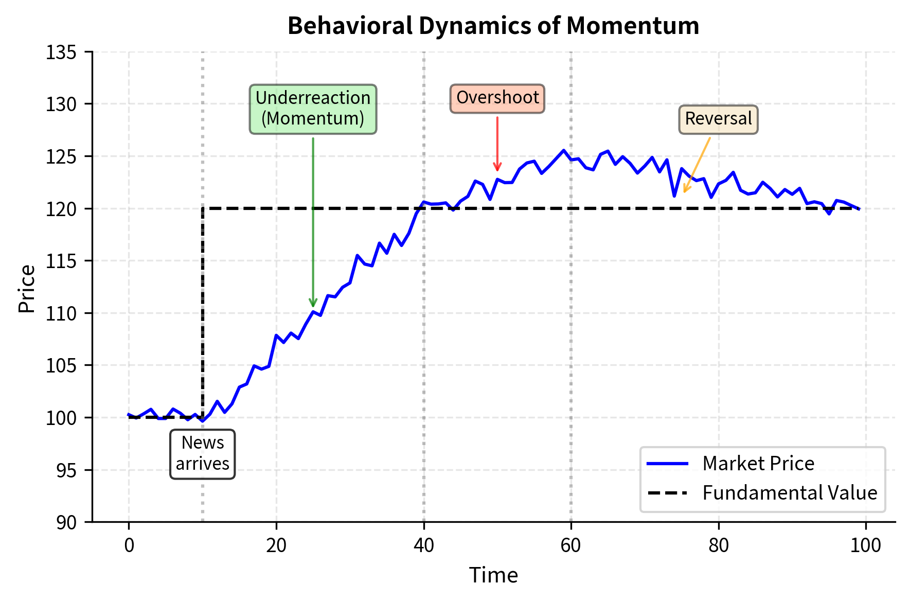
The foundation of time-series momentum rests on a deceptively simple observation: recent price direction tends to persist. Before we formalize this intuition, consider why such persistence might exist. When new information enters the market, perhaps an unexpected earnings surprise or a shift in monetary policy, prices do not instantly jump to their new equilibrium value. Instead, the adjustment unfolds gradually as different market participants learn about, interpret, and act upon the news. This gradual adjustment creates a window during which prices exhibit directional persistence, and momentum strategies seek to profit from this window.

The simplest time-series momentum signal compares an asset's current price to its price $k$ periods ago. This comparison answers a fundamental question: has the asset been trending upward or downward over the recent past? If we denote the price at time $t$ as $P_t$ , the momentum signal is:

\text{TSMOM}_t = \text{sign}(P_t - P_{t-k}) = \text{sign}(r_{t-k,t})

where:

$P_t$ : price of the asset at time $t$
$P_{t-k}$ : price of the asset $k$ periods ago
$r_{t-k,t}$ : cumulative return over the lookback period
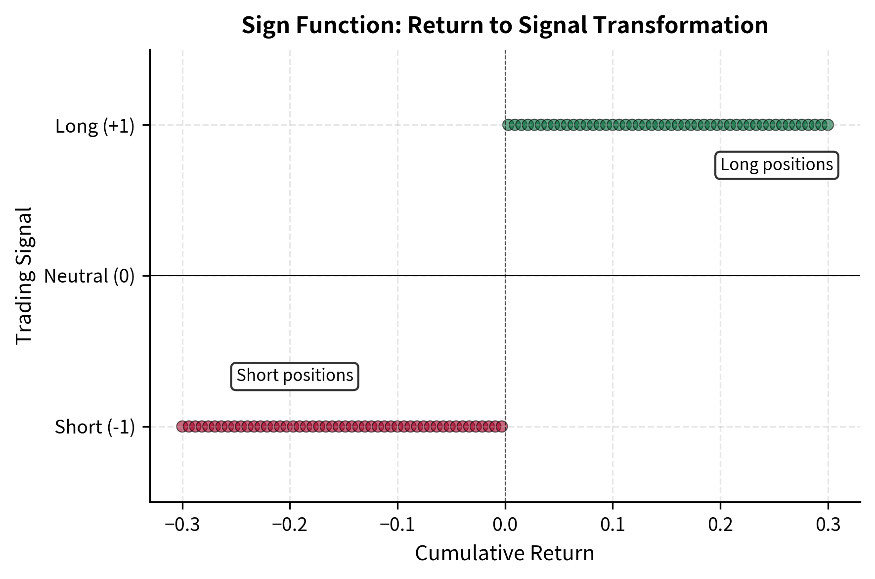
$\text{sign}(\cdot)$ : function returning $+1$ if positive, $-1$ if negative, and $0$ if zero

The sign function transforms the continuous return into a discrete trading signal. A positive signal indicates a long position, while a negative signal indicates a short position. This binary transformation reflects the core philosophy of trend following: we care primarily about the direction of the trend rather than its magnitude. A stock that rose 5% over the past year receives the same long signal as one that rose 50%, because both have demonstrated positive momentum.

Out[3]:

Visualization

The sign function transforms continuous returns into discrete trading signals. Positive returns generate long signals (+1), negative returns generate short signals (-1), creating a binary decision rule for trend following.

In practice, however, raw price comparisons can generate noisy signals that whipsaw between long and short positions during sideways markets. You often use moving averages to smooth noise and generate more stable signals. The smoothing process filters out short-term fluctuations while preserving the underlying trend direction. The dual moving average crossover represents one of the most popular implementations, comparing a fast moving average with a short lookback period to a slow moving average with a longer lookback period:

\text{Signal}_t = \text{sign}(\text{MA}_t^{\text{fast}} - \text{MA}_t^{\text{slow}})

where:

$\text{MA}_t^{\text{fast}}$ : moving average value with a short lookback period
$\text{MA}_t^{\text{slow}}$ : moving average value with a long lookback period
$\text{sign}(\cdot)$ : function returning $+1$ if positive, $-1$ if negative, and $0$ otherwise

The intuition behind this signal is elegant: the fast moving average represents recent price momentum, while the slow moving average represents the longer-term price equilibrium. When the fast average crosses above the slow average, it suggests that short-term momentum has turned positive relative to the longer-term baseline. This crossover often signals a shift in market sentiment or a fundamental change in the asset's supply and demand dynamics. Conversely, when the fast average crosses below the slow average, it indicates deteriorating short-term momentum and suggests the trend may be reversing.

The simple moving average (SMA) calculates the arithmetic mean of prices over a lookback window $n$ , treating each observation within the window equally:

\text{MA}_t^n = \frac{1}{n}\sum_{i=0}^{n-1} P_{t-i}

where:

$\text{MA}_t^n$ : simple moving average at time $t$ with lookback $n$
$P_{t-i}$ : asset price at lag $i$
$n$ : number of periods in the moving average window

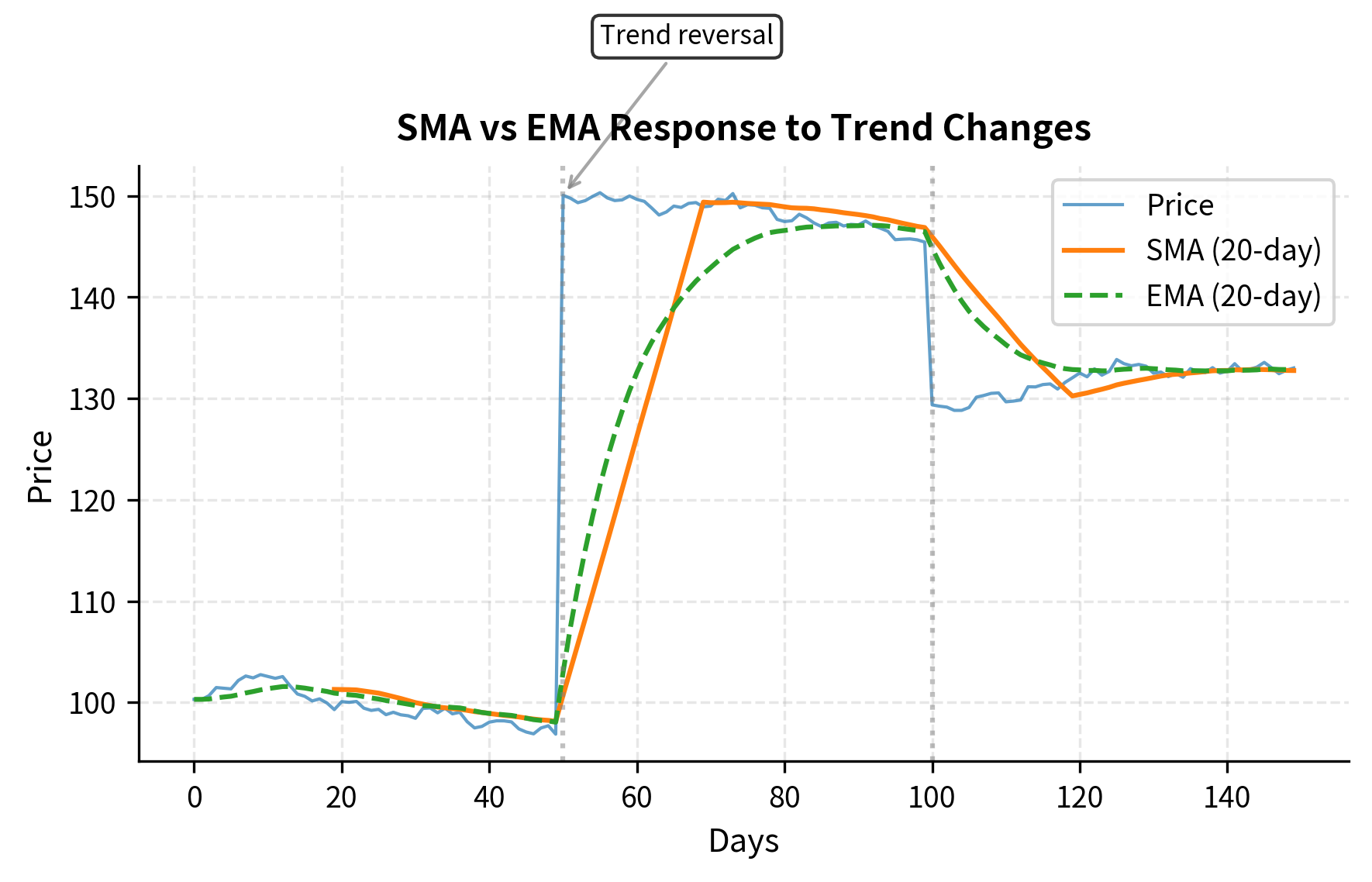
By weighting all prices in the window equally with coefficient $1/n$ , this formula filters out high-frequency noise but introduces a deliberate lag. The average reacts more slowly to new price changes compared to the raw price series because each new observation only contributes $1/n$ of the total average value. This lag represents a tradeoff inherent in all smoothing techniques: greater noise reduction comes at the cost of slower signal response. For a 50-day moving average, today's price contributes only 2% of the average value, meaning the average responds gradually to even substantial price movements.

While simple moving averages provide effective smoothing, you might prefer alternatives that give more weight to recent observations. Exponential moving averages (EMAs) provide such an alternative, assigning exponentially decaying weights to historical prices:

\text{EMA}_t = \alpha P_t + (1-\alpha)\text{EMA}_{t-1}

where:

$\alpha$ : smoothing factor, typically calculated as $2/(n+1)$
$n$ : effective span or lookback period
$P_t$ : current asset price
$\text{EMA}_{t-1}$ : value of the exponential moving average in the previous period

This recursive formulation reveals the elegant structure of the EMA. The formula updates the average by combining two components: the new information $\alpha P_t$ representing today's price contribution, and the accumulated history $(1-\alpha)\text{EMA}_{t-1}$ carrying forward the weighted sum of all previous prices. The smoothing factor $\alpha$ determines the relative importance of new versus old information. A larger $\alpha$ value creates a more responsive average that tracks price changes closely, while a smaller $\alpha$ produces a smoother average that emphasizes historical prices. The exponential weighting scheme assigns geometrically declining weights to older observations, so the average maintains a fading memory of the entire price series while remaining more responsive to recent trend changes than a simple moving average of equivalent span.

Out[4]:

Visualization

Comparison of Simple Moving Average (SMA) and Exponential Moving Average (EMA) with equivalent 20-day spans. The EMA responds more quickly to price changes due to its exponentially decaying weights, while the SMA provides smoother but lagged signals.

Implementing Moving Average CrossoversLink Copied

Let's implement a dual moving average crossover strategy on equity index data. We'll use a 50-day fast moving average and a 200-day slow moving average, a popular combination known as the golden cross (when fast crosses above slow) and death cross (when fast crosses below slow).

In[5]:

Code

import numpy as np
import pandas as pd

# import yfinance as yf
from datetime import datetime

# Download S&P 500 ETF data
# end_date = datetime.now()
# start_date = end_date - timedelta(days=365*10)
# spy = yf.download('SPY', start=start_date, end=end_date, progress=False)
# prices = spy['Close'].squeeze()

# Generate synthetic data for demonstration
np.random.seed(42)
dates = pd.date_range(end=datetime.now(), periods=252 * 10, freq="B")
returns = np.random.normal(0.0004, 0.012, len(dates))  # Drift + Noise
prices = pd.Series(100 * (1 + returns).cumprod(), index=dates)

# Calculate moving averages
ma_fast = prices.rolling(window=50).mean()
ma_slow = prices.rolling(window=200).mean()

# Generate signals: 1 for long, -1 for short/flat
signal = np.where(ma_fast > ma_slow, 1, -1)
signal = pd.Series(signal, index=prices.index)

import numpy as np
import pandas as pd

# import yfinance as yf
from datetime import datetime

# Download S&P 500 ETF data
# end_date = datetime.now()
# start_date = end_date - timedelta(days=365*10)
# spy = yf.download('SPY', start=start_date, end=end_date, progress=False)
# prices = spy['Close'].squeeze()

# Generate synthetic data for demonstration
np.random.seed(42)
dates = pd.date_range(end=datetime.now(), periods=252 * 10, freq="B")
returns = np.random.normal(0.0004, 0.012, len(dates))  # Drift + Noise
prices = pd.Series(100 * (1 + returns).cumprod(), index=dates)

# Calculate moving averages
ma_fast = prices.rolling(window=50).mean()
ma_slow = prices.rolling(window=200).mean()

# Generate signals: 1 for long, -1 for short/flat
signal = np.where(ma_fast > ma_slow, 1, -1)
signal = pd.Series(signal, index=prices.index)

Out[6]:

Visualization

Line chart showing SPY price with two moving average lines and shaded regions for long and short signals. — S&P 500 ETF price tracked by 50-day and 200-day moving averages. The crossovers successfully identify primary trends, with the strategy remaining long during sustained rallies while signaling defensive shifts during major corrections.

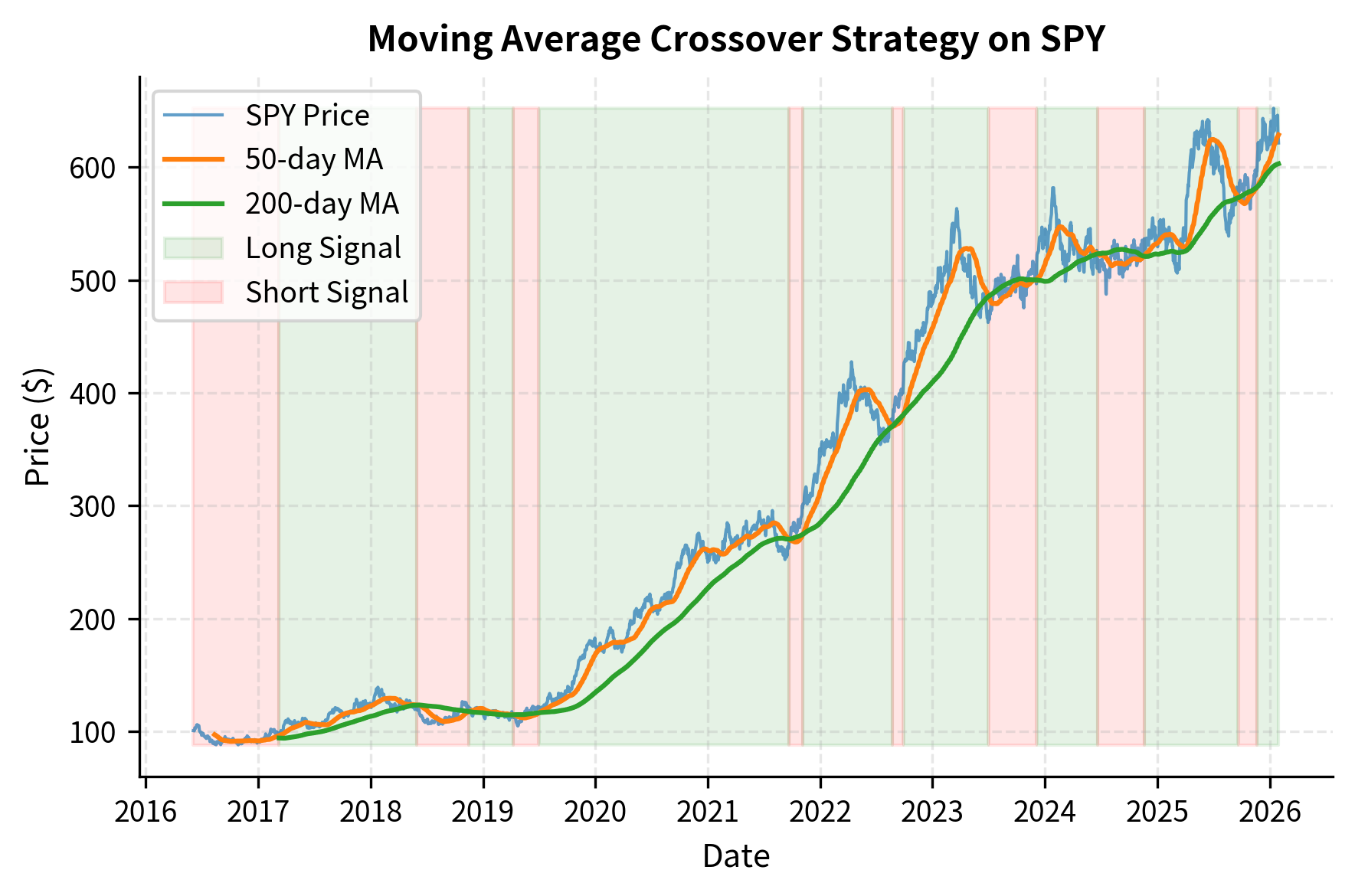
The shaded regions reveal how the strategy positions itself during different market regimes. During sustained uptrends, the fast moving average stays above the slow, keeping the strategy long. During corrections, the crossover generates a short or flat signal.

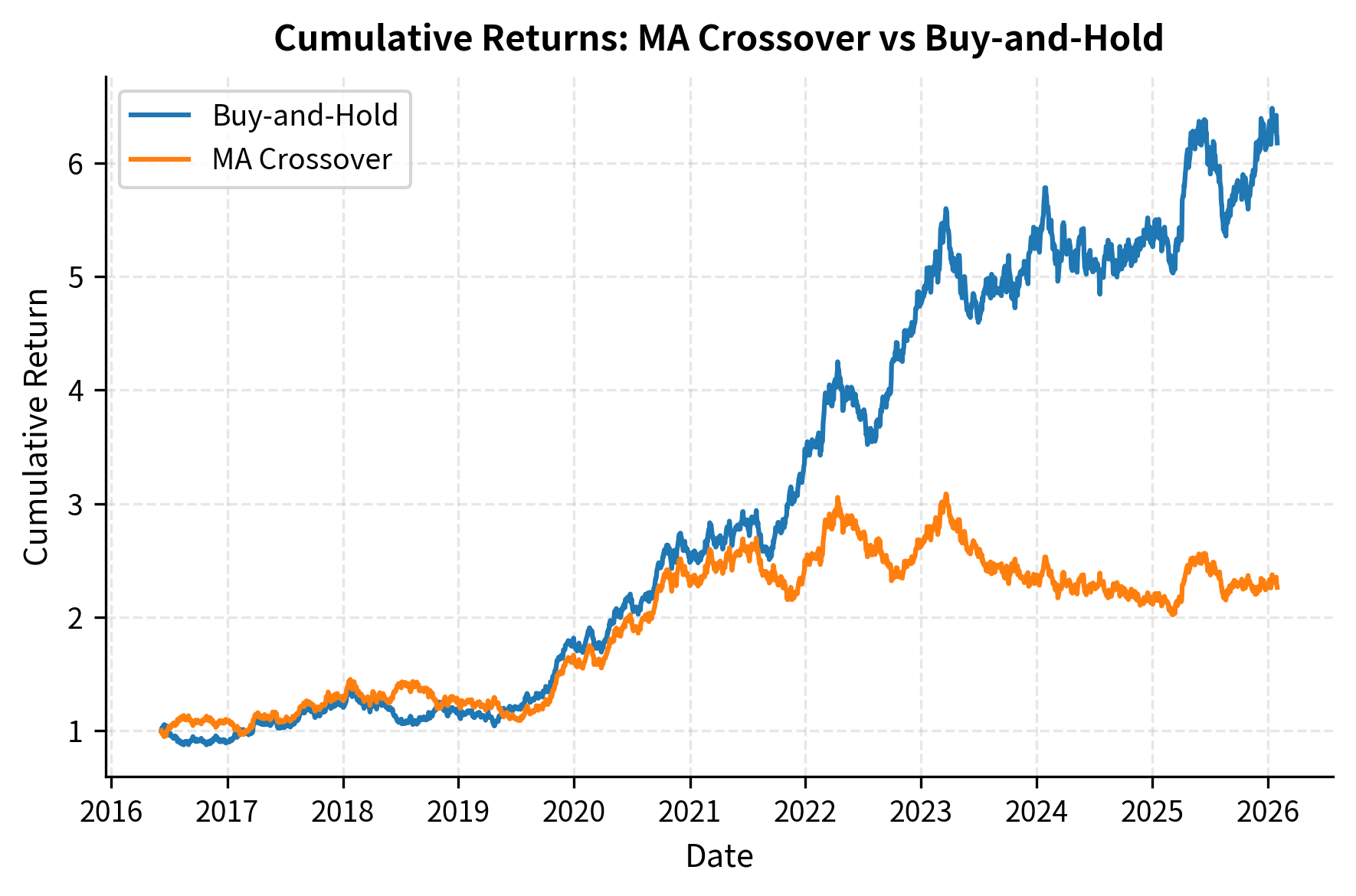
Now let's calculate the strategy's returns and compare them to buy-and-hold:

In[7]:

Code

# Calculate daily returns
daily_returns = prices.pct_change()

# Strategy returns: signal is lagged by 1 day to avoid look-ahead bias
strategy_returns = signal.shift(1) * daily_returns

# Calculate cumulative returns
cumulative_market = (1 + daily_returns).cumprod()
cumulative_strategy = (1 + strategy_returns).cumprod()


# Performance metrics
def calculate_metrics(returns, periods_per_year=252):
    """Calculate key performance metrics for a return series."""
    returns = returns.dropna()
    total_return = (1 + returns).prod() - 1
    years = len(returns) / periods_per_year
    ann_return = (1 + total_return) ** (1 / years) - 1
    ann_vol = returns.std() * np.sqrt(periods_per_year)
    sharpe = ann_return / ann_vol if ann_vol > 0 else 0

    # Maximum drawdown
    cumulative = (1 + returns).cumprod()
    rolling_max = cumulative.expanding().max()
    drawdowns = cumulative / rolling_max - 1
    max_dd = drawdowns.min()

    return {
        "Total Return": total_return,
        "Annualized Return": ann_return,
        "Annualized Volatility": ann_vol,
        "Sharpe Ratio": sharpe,
        "Max Drawdown": max_dd,
    }


market_metrics = calculate_metrics(daily_returns)
strategy_metrics = calculate_metrics(strategy_returns)

# Calculate daily returns
daily_returns = prices.pct_change()

# Strategy returns: signal is lagged by 1 day to avoid look-ahead bias
strategy_returns = signal.shift(1) * daily_returns

# Calculate cumulative returns
cumulative_market = (1 + daily_returns).cumprod()
cumulative_strategy = (1 + strategy_returns).cumprod()


# Performance metrics
def calculate_metrics(returns, periods_per_year=252):
    """Calculate key performance metrics for a return series."""
    returns = returns.dropna()
    total_return = (1 + returns).prod() - 1
    years = len(returns) / periods_per_year
    ann_return = (1 + total_return) ** (1 / years) - 1
    ann_vol = returns.std() * np.sqrt(periods_per_year)
    sharpe = ann_return / ann_vol if ann_vol > 0 else 0

    # Maximum drawdown
    cumulative = (1 + returns).cumprod()
    rolling_max = cumulative.expanding().max()
    drawdowns = cumulative / rolling_max - 1
    max_dd = drawdowns.min()

    return {
        "Total Return": total_return,
        "Annualized Return": ann_return,
        "Annualized Volatility": ann_vol,
        "Sharpe Ratio": sharpe,
        "Max Drawdown": max_dd,
    }


market_metrics = calculate_metrics(daily_returns)
strategy_metrics = calculate_metrics(strategy_returns)

Out[8]:

Console

Performance Comparison: Moving Average Crossover vs Buy-and-Hold
=================================================================
Metric                          Buy-and-Hold       MA Crossover
-----------------------------------------------------------------
Total Return                         517.6%            126.2%
Annualized Return                     20.0%              8.5%
Annualized Volatility                   0.19               0.19
Sharpe Ratio                            1.07               0.45
Max Drawdown                         -24.6%            -34.5%

The metrics comparison highlights the trade-offs of the strategy. While the Buy-and-Hold approach tracks the market's total return, the Moving Average Crossover strategy aims to improve the Sharpe Ratio by sidestepping major drawdowns, albeit often at the cost of lower total returns during strong bull markets.

Out[9]:

Visualization

Line chart comparing cumulative returns of MA crossover strategy versus buy-and-hold benchmark. — Cumulative returns comparison between the moving average crossover strategy and buy-and-hold. The trend-following approach provides a smoother equity curve by reducing drawdown depth, though it exhibits performance lag during strong bull markets.

Key ParametersLink Copied

The key parameters for the Moving Average Crossover strategy are:

Fast Window: The lookback period for the short-term moving average (e.g., 50 days). Shorter windows make the strategy more responsive but prone to false signals.
Slow Window: The lookback period for the long-term baseline (e.g., 200 days). Longer windows filter more noise but increase lag.
Regime: The market state (trending vs. mean-reverting) heavily influences performance. Crossovers perform best in sustained trends.

Breakout StrategiesLink Copied

Breakout strategies represent another powerful implementation of time-series momentum, grounded in a different but related intuition. Rather than using moving average crossovers, breakout systems enter positions when prices exceed recent highs or lows. The underlying premise is that price extremes carry informational content: when an asset reaches a new high, it signals that buyers have overwhelmed sellers at all previously established price levels, suggesting strong demand that may persist. Conversely, a new low indicates that selling pressure has broken through all previous support levels.

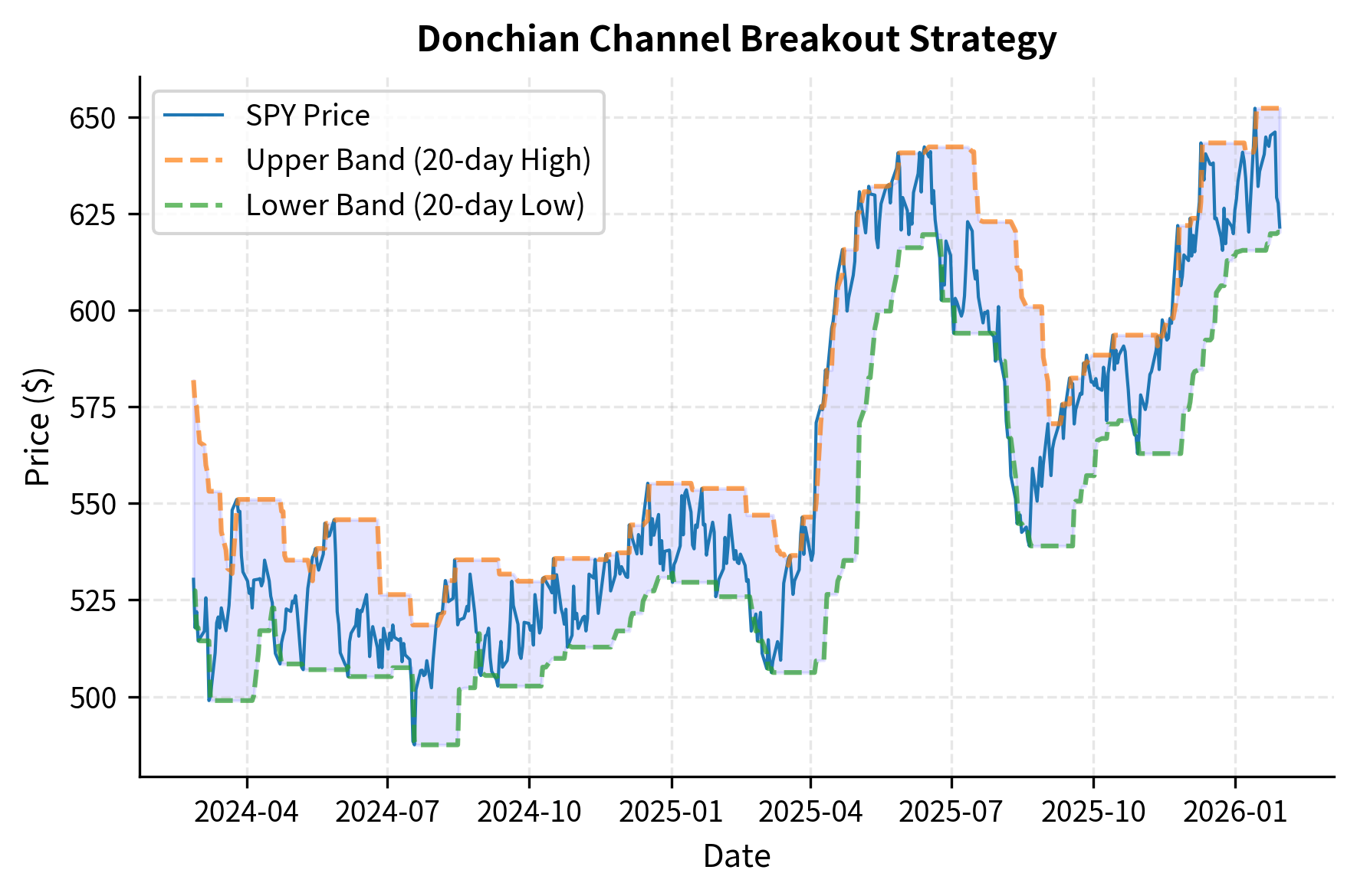
The classic Donchian channel strategy, popularized by the famous "Turtle Traders" in the 1980s, operationalizes this intuition by buying when price breaks above the highest high of the past $n$ days and selling when price breaks below the lowest low. The Turtle Traders demonstrated that this systematic approach, when combined with proper position sizing and risk management, could generate substantial profits across diverse futures markets.

The Donchian channel defines dynamic support and resistance levels based on recent price extremes:

\begin{aligned} \text{Upper\_Band}_t &= \max(P_{t-1}, P_{t-2}, \ldots, P_{t-n}) \\ \text{Lower\_Band}_t &= \min(P_{t-1}, P_{t-2}, \ldots, P_{t-n}) \end{aligned}

where:

$\text{Upper\_Band}_t$ : highest price over the past $n$ periods
$\text{Lower\_Band}_t$ : lowest price over the past $n$ periods
$P_{t-i}$ : asset price $i$ periods ago
$n$ : lookback window size

These formulas create a price channel that contains all price action over the lookback window. The upper band represents the resistance level that buyers have been unable to breach, while the lower band represents the support level that sellers have been unable to break. When price finally moves outside this channel, it suggests a potential shift in the market's supply and demand equilibrium.

A long entry occurs when $P_t > \text{Upper\_Band}_t$ , indicating that today's price has exceeded all prices in the lookback window. This breakout above resistance suggests that new buyers have entered the market or that existing buyers have become more aggressive, potentially initiating an upward trend. A short entry occurs when $P_t < \text{Lower\_Band}_t$ , indicating that today's price has fallen below all recent support levels. This breakout logic assumes that prices reaching new extremes signal a fundamental shift in market dynamics that is likely to persist as other market participants recognize and react to the new price regime.

In[10]:

Code

# Donchian Channel breakout strategy
lookback = 20  # 20-day breakout

upper_band = prices.rolling(window=lookback).max().shift(1)
lower_band = prices.rolling(window=lookback).min().shift(1)

# Generate signals
breakout_signal = pd.Series(0.0, index=prices.index)
position = 0

for i in range(lookback, len(prices)):
    if prices.iloc[i] > upper_band.iloc[i]:
        position = 1  # Long breakout
    elif prices.iloc[i] < lower_band.iloc[i]:
        position = -1  # Short breakout
    breakout_signal.iloc[i] = position

# Calculate returns
breakout_returns = breakout_signal.shift(1) * daily_returns
cumulative_breakout = (1 + breakout_returns).cumprod()

# Donchian Channel breakout strategy
lookback = 20  # 20-day breakout

upper_band = prices.rolling(window=lookback).max().shift(1)
lower_band = prices.rolling(window=lookback).min().shift(1)

# Generate signals
breakout_signal = pd.Series(0.0, index=prices.index)
position = 0

for i in range(lookback, len(prices)):
    if prices.iloc[i] > upper_band.iloc[i]:
        position = 1  # Long breakout
    elif prices.iloc[i] < lower_band.iloc[i]:
        position = -1  # Short breakout
    breakout_signal.iloc[i] = position

# Calculate returns
breakout_returns = breakout_signal.shift(1) * daily_returns
cumulative_breakout = (1 + breakout_returns).cumprod()

Out[11]:

Visualization

Price chart with Donchian channel bands and signal markers for breakout entries. — Donchian Channel breakout strategy showing the upper and lower bands based on 20-day highs and lows. The strategy captures trending moves as prices break through established resistance, staying invested during sustained price extensions.

Key ParametersLink Copied

The key parameters for Breakout strategies are:

Lookback Period ( $n$ ): The window for determining the breakout levels (e.g., 20 days).
Upper/Lower Bands: The highest high and lowest low over the lookback period, which serve as dynamic support and resistance levels.

CTA Strategies and Multi-Asset Trend FollowingLink Copied

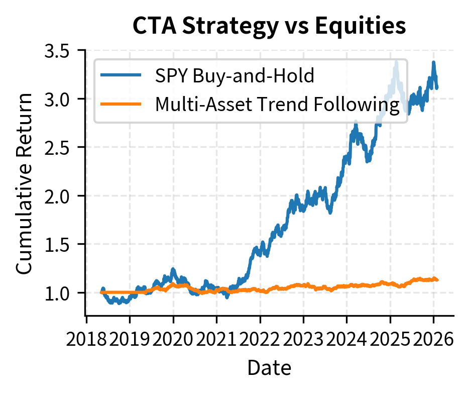
Commodity Trading Advisors (CTAs) are managed futures funds that primarily employ trend-following strategies across a diversified portfolio of futures contracts. The power of CTA strategies comes from combining trend signals across multiple uncorrelated asset classes: equity indices, government bonds, currencies, commodities, and interest rates.

The key insight is that while any single trend signal may fail, combining signals across 50 to 100 futures markets with low correlation to each other produces a more stable return stream. The strategy also benefits from the ability to profit in both rising and falling markets, providing valuable diversification during equity bear markets.

A typical CTA strategy involves several components:

Signal generation: Each market receives a trend signal (e.g., moving average crossover, momentum score, or breakout)
Volatility scaling: Position sizes are inversely proportional to recent volatility, so more volatile markets receive smaller positions
Risk allocation: Capital is allocated across asset classes and individual markets based on target risk contribution
Portfolio construction: Final positions combine signals, volatility scaling, and risk budgets

Let's implement a simplified multi-asset trend following system:

In[12]:

Code

from datetime import datetime, timedelta

# Download futures proxy data for multiple asset classes
tickers = {
    "SPY": "Equities",  # S&P 500
    "TLT": "Bonds",  # Long-term Treasuries
    "GLD": "Commodities",  # Gold
    "UUP": "Currencies",  # US Dollar Index
}

end_date = datetime.now()
start_date = end_date - timedelta(days=365 * 8)

# data = {}
# for ticker, asset_class in tickers.items():
#     df = yf.download(ticker, start=start_date, end=end_date, progress=False)
#     data[ticker] = df['Close'].squeeze()

# prices_df = pd.DataFrame(data)

# Generate synthetic data for demonstration
np.random.seed(42)
dates = pd.date_range(end=datetime.now(), periods=252 * 8, freq="B")
data = {
    ticker: 100 * (1 + np.random.normal(0.0002, 0.01, len(dates))).cumprod()
    for ticker in tickers
}
prices_df = pd.DataFrame(data, index=dates)
returns_df = prices_df.pct_change()

# Calculate momentum signals for each asset
lookback_signal = 252  # 12-month momentum
lookback_vol = 63  # 3-month volatility for scaling

signals = pd.DataFrame(index=prices_df.index, columns=prices_df.columns)
vol_scaled_signals = pd.DataFrame(
    index=prices_df.index, columns=prices_df.columns
)

for ticker in tickers.keys():
    # 12-month momentum signal
    momentum = prices_df[ticker] / prices_df[ticker].shift(lookback_signal) - 1
    signals[ticker] = np.sign(momentum)

    # Volatility scaling: target 10% annual vol per position
    realized_vol = returns_df[ticker].rolling(lookback_vol).std() * np.sqrt(252)
    target_vol = 0.10
    vol_scalar = target_vol / realized_vol
    vol_scalar = vol_scalar.clip(upper=2.0)  # Cap leverage at 2x

    vol_scaled_signals[ticker] = signals[ticker] * vol_scalar

# Equal-weight portfolio of vol-scaled signals
n_assets = len(tickers)
portfolio_returns = (vol_scaled_signals.shift(1) * returns_df).sum(
    axis=1
) / n_assets
cumulative_cta = (1 + portfolio_returns).cumprod()

from datetime import datetime, timedelta

# Download futures proxy data for multiple asset classes
tickers = {
    "SPY": "Equities",  # S&P 500
    "TLT": "Bonds",  # Long-term Treasuries
    "GLD": "Commodities",  # Gold
    "UUP": "Currencies",  # US Dollar Index
}

end_date = datetime.now()
start_date = end_date - timedelta(days=365 * 8)

# data = {}
# for ticker, asset_class in tickers.items():
#     df = yf.download(ticker, start=start_date, end=end_date, progress=False)
#     data[ticker] = df['Close'].squeeze()

# prices_df = pd.DataFrame(data)

# Generate synthetic data for demonstration
np.random.seed(42)
dates = pd.date_range(end=datetime.now(), periods=252 * 8, freq="B")
data = {
    ticker: 100 * (1 + np.random.normal(0.0002, 0.01, len(dates))).cumprod()
    for ticker in tickers
}
prices_df = pd.DataFrame(data, index=dates)
returns_df = prices_df.pct_change()

# Calculate momentum signals for each asset
lookback_signal = 252  # 12-month momentum
lookback_vol = 63  # 3-month volatility for scaling

signals = pd.DataFrame(index=prices_df.index, columns=prices_df.columns)
vol_scaled_signals = pd.DataFrame(
    index=prices_df.index, columns=prices_df.columns
)

for ticker in tickers.keys():
    # 12-month momentum signal
    momentum = prices_df[ticker] / prices_df[ticker].shift(lookback_signal) - 1
    signals[ticker] = np.sign(momentum)

    # Volatility scaling: target 10% annual vol per position
    realized_vol = returns_df[ticker].rolling(lookback_vol).std() * np.sqrt(252)
    target_vol = 0.10
    vol_scalar = target_vol / realized_vol
    vol_scalar = vol_scalar.clip(upper=2.0)  # Cap leverage at 2x

    vol_scaled_signals[ticker] = signals[ticker] * vol_scalar

# Equal-weight portfolio of vol-scaled signals
n_assets = len(tickers)
portfolio_returns = (vol_scaled_signals.shift(1) * returns_df).sum(
    axis=1
) / n_assets
cumulative_cta = (1 + portfolio_returns).cumprod()

Out[13]:

Visualization

Line chart comparing CTA strategy cumulative returns to SPY buy-and-hold. — Cumulative returns of the multi-asset trend following strategy compared to the S&P 500. The trend-following strategy demonstrates consistent growth with distinct drawdown characteristics, illustrating the diversification benefits of multi-asset allocation.

Time series of rolling correlation between CTA returns and equity returns. — Rolling 12-month correlation between the CTA strategy and equities. The correlation frequently drops toward or below zero during periods of market stress, providing structural diversification when traditional assets decline.

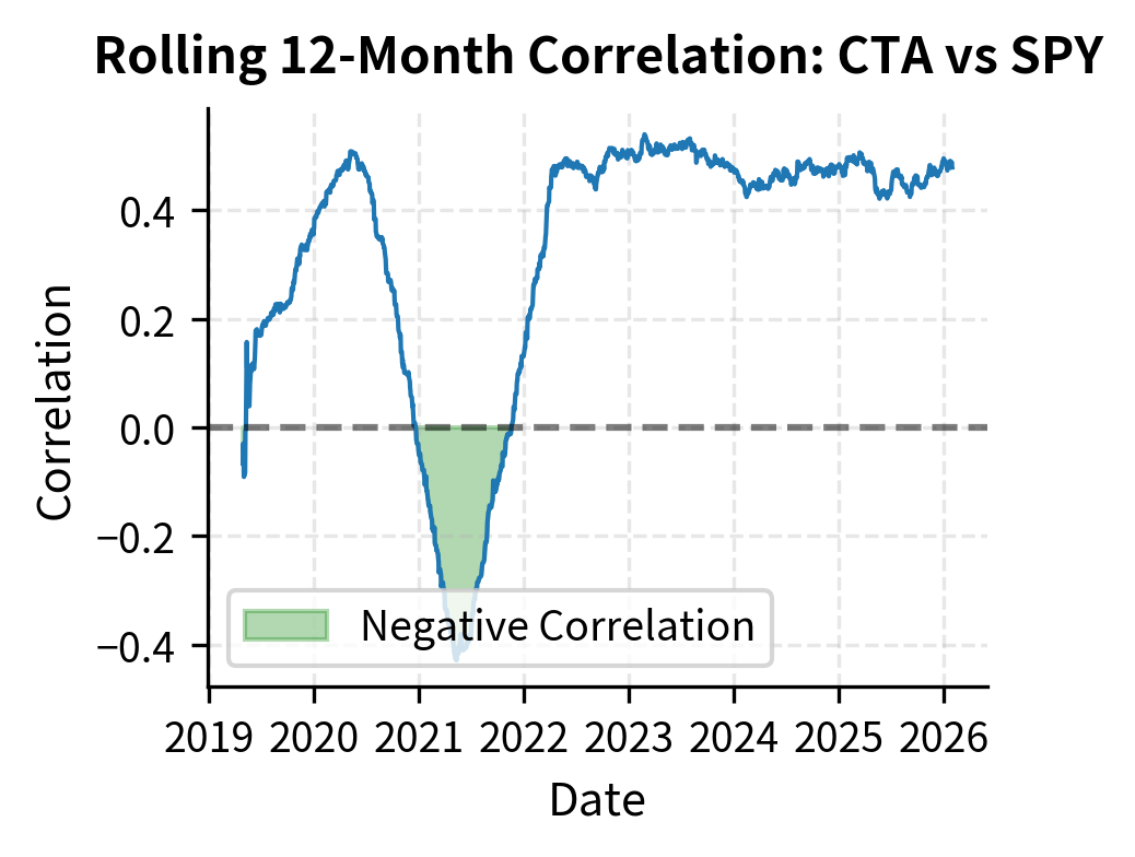
The rolling correlation chart reveals why institutional investors value trend-following strategies: during market stress periods, the correlation often turns negative, providing protection precisely when diversification is most needed. This "crisis alpha" property stems from the strategy's ability to go short during sustained market declines.

Key ParametersLink Copied

The key parameters for the Multi-Asset CTA strategy are:

Signal Lookback: The period for measuring momentum (e.g., 12 months).
Volatility Lookback: The window for estimating asset volatility to scale positions (e.g., 3 months).
Target Volatility: The desired annualized volatility level for each position or the portfolio.
Leverage Cap: Maximum leverage allowed per position to prevent excessive risk.

Cross-Sectional MomentumLink Copied

While time-series momentum compares an asset to its own history, cross-sectional momentum takes a fundamentally different approach: it ranks assets relative to their peers and takes long positions in recent winners while shorting recent losers. The distinction is subtle but important. Time-series momentum asks, "Has this asset been going up?" Cross-sectional momentum asks, "Has this asset been going up more than other similar assets?" This relative comparison exploits a different source of return persistence, one related to the dispersion in performance across assets rather than the absolute direction of any single asset.

This approach was documented in the seminal work by Jegadeesh and Titman (1993), who showed that buying stocks that performed well over the past 3 to 12 months and selling stocks that performed poorly generates significant excess returns. Their findings challenged the notion of market efficiency by demonstrating a simple, mechanical trading rule that produced consistent profits.

The Jegadeesh-Titman FrameworkLink Copied

The classic cross-sectional momentum strategy involves three parameters that determine how the portfolio is constructed and managed:

Formation period ( $J$ ): The lookback window for ranking stocks (typically 3, 6, or 12 months)
Holding period ( $K$ ): How long positions are held (typically 3, 6, or 12 months)
Skip period: Often 1 month is skipped between formation and holding to avoid short-term reversal effects

The formation period defines how we measure past performance, recognizing that momentum persistence varies across different time horizons. The holding period determines how long we maintain positions before rebalancing, balancing the tradeoff between capturing momentum profits and incurring transaction costs. The skip period addresses a well-documented empirical finding: stocks exhibit short-term reversal in the weeks immediately following extreme returns, so skipping a month between ranking and trading improves strategy performance.

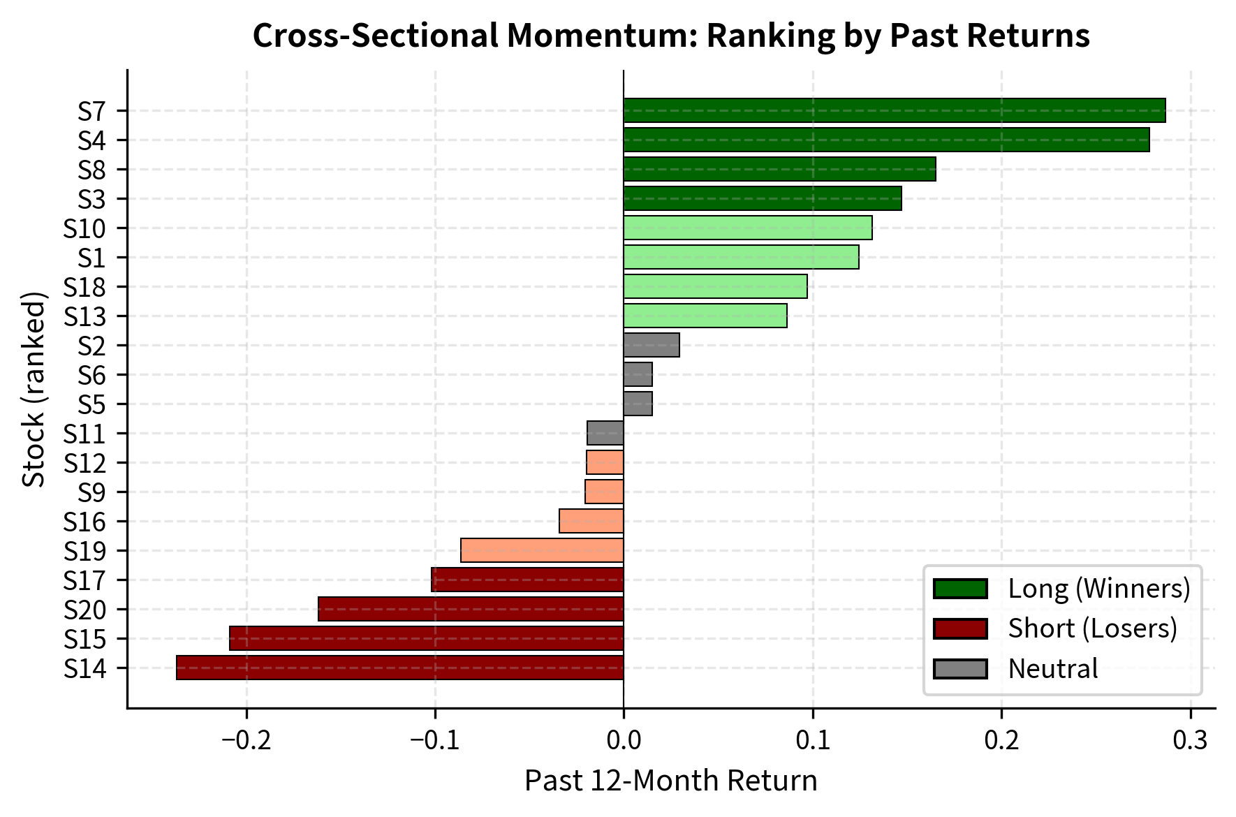
At each rebalancing date, stocks are ranked by their formation period returns and sorted into decile portfolios. The momentum portfolio goes long the top decile (winners) and short the bottom decile (losers).

The momentum factor return captures the performance spread between recent winners and recent losers:

r_{\text{MOM},t} = r_{\text{Winners},t} - r_{\text{Losers},t}

where:

$r_{\text{MOM},t}$ : return of the long-short momentum factor at time $t$
$r_{\text{Winners},t}$ : return of the top decile (winner) portfolio
$r_{\text{Losers},t}$ : return of the bottom decile (loser) portfolio

This long-short construction creates a dollar-neutral portfolio with equal long and short exposure. The design isolates the performance spread, often interpreted as alpha, between winners and losers while hedging out the market's general direction, or beta. If the market rises 10%, both the winner and loser portfolios will likely rise, but the momentum return captures only the difference in how much each rose. This neutralization makes momentum returns relatively independent of market direction, though as we will see later, this independence breaks down during sharp market reversals.

Empirically, this spread has averaged 1% per month in US equities, though returns vary significantly over time and across markets. The magnitude and consistency of this premium attracted substantial academic attention and practical capital to momentum-based strategies.

Out[14]:

Visualization

Cross-sectional momentum ranking of assets by past performance. The significant return dispersion between winners and losers highlights the opportunity for capturing a momentum premium through long-short positioning.

Implementing Cross-Sectional MomentumLink Copied

Let's implement a cross-sectional momentum strategy on a universe of liquid US stocks:

In[15]:

Code

# Download a universe of large-cap stocks
stock_universe = [
    "AAPL",
    "MSFT",
    "GOOGL",
    "AMZN",
    "META",
    "NVDA",
    "TSLA",
    "JPM",
    "V",
    "JNJ",
    "WMT",
    "PG",
    "MA",
    "HD",
    "DIS",
    "NFLX",
    "PYPL",
    "ADBE",
    "CRM",
    "INTC",
    "CSCO",
    "PFE",
    "ABT",
    "MRK",
    "KO",
]

end_date = datetime.now()
start_date = end_date - timedelta(days=365 * 6)

# stock_data = {}
# for ticker in stock_universe:
#     # ... download logic ...
#     pass
# stock_prices = pd.DataFrame(stock_data)

# Generate synthetic data for demonstration
np.random.seed(42)
dates = pd.date_range(
    end=pd.Timestamp.now().normalize(), periods=252 * 6, freq="B"
)
# Create correlated stock data
market_factor = np.random.normal(0.0005, 0.01, len(dates))
stock_data = {}
for ticker in stock_universe:
    noise = np.random.normal(0, 0.02, len(dates))
    ret = 0.5 * market_factor + 0.5 * noise
    stock_data[ticker] = 100 * (1 + ret).cumprod()
stock_prices = pd.DataFrame(stock_data, index=dates)
stock_returns = stock_prices.pct_change()

# Download a universe of large-cap stocks
stock_universe = [
    "AAPL",
    "MSFT",
    "GOOGL",
    "AMZN",
    "META",
    "NVDA",
    "TSLA",
    "JPM",
    "V",
    "JNJ",
    "WMT",
    "PG",
    "MA",
    "HD",
    "DIS",
    "NFLX",
    "PYPL",
    "ADBE",
    "CRM",
    "INTC",
    "CSCO",
    "PFE",
    "ABT",
    "MRK",
    "KO",
]

end_date = datetime.now()
start_date = end_date - timedelta(days=365 * 6)

# stock_data = {}
# for ticker in stock_universe:
#     # ... download logic ...
#     pass
# stock_prices = pd.DataFrame(stock_data)

# Generate synthetic data for demonstration
np.random.seed(42)
dates = pd.date_range(
    end=pd.Timestamp.now().normalize(), periods=252 * 6, freq="B"
)
# Create correlated stock data
market_factor = np.random.normal(0.0005, 0.01, len(dates))
stock_data = {}
for ticker in stock_universe:
    noise = np.random.normal(0, 0.02, len(dates))
    ret = 0.5 * market_factor + 0.5 * noise
    stock_data[ticker] = 100 * (1 + ret).cumprod()
stock_prices = pd.DataFrame(stock_data, index=dates)
stock_returns = stock_prices.pct_change()

In[16]:

Code

# Cross-sectional momentum parameters
formation_period = 252  # 12-month lookback
skip_period = 21  # Skip 1 month
n_long = 5  # Number of stocks to go long
n_short = 5  # Number of stocks to go short

# Calculate momentum scores (12-month returns)
momentum_scores = stock_prices.pct_change(formation_period)

# Rebalance monthly
rebalance_dates = stock_returns.resample("BM").last().index

portfolio_returns = []
holdings_history = []

for i, date in enumerate(rebalance_dates[:-1]):
    # Get momentum scores as of skip_period days before rebalance
    try:
        score_date = stock_returns.index[
            stock_returns.index.get_loc(date) - skip_period
        ]
    except (KeyError, IndexError):
        continue

    scores = momentum_scores.loc[score_date].dropna()
    if len(scores) < n_long + n_short:
        continue

    # Rank and select winners/losers
    ranked = scores.sort_values(ascending=False)
    winners = ranked.head(n_long).index.tolist()
    losers = ranked.tail(n_short).index.tolist()

    # Get returns for holding period (next month)
    next_date = rebalance_dates[i + 1]
    period_returns = stock_returns.loc[date:next_date]

    if len(period_returns) > 1:
        # Equal-weight long winners, short losers
        long_ret = period_returns[winners].mean(axis=1).sum()
        short_ret = period_returns[losers].mean(axis=1).sum()
        mom_return = long_ret - short_ret

        portfolio_returns.append(
            {
                "date": next_date,
                "return": mom_return,
                "long_return": long_ret,
                "short_return": short_ret,
                "winners": winners,
                "losers": losers,
            }
        )

momentum_df = pd.DataFrame(portfolio_returns)
momentum_df.set_index("date", inplace=True)

# Cross-sectional momentum parameters
formation_period = 252  # 12-month lookback
skip_period = 21  # Skip 1 month
n_long = 5  # Number of stocks to go long
n_short = 5  # Number of stocks to go short

# Calculate momentum scores (12-month returns)
momentum_scores = stock_prices.pct_change(formation_period)

# Rebalance monthly
rebalance_dates = stock_returns.resample("BM").last().index

portfolio_returns = []
holdings_history = []

for i, date in enumerate(rebalance_dates[:-1]):
    # Get momentum scores as of skip_period days before rebalance
    try:
        score_date = stock_returns.index[
            stock_returns.index.get_loc(date) - skip_period
        ]
    except (KeyError, IndexError):
        continue

    scores = momentum_scores.loc[score_date].dropna()
    if len(scores) < n_long + n_short:
        continue

    # Rank and select winners/losers
    ranked = scores.sort_values(ascending=False)
    winners = ranked.head(n_long).index.tolist()
    losers = ranked.tail(n_short).index.tolist()

    # Get returns for holding period (next month)
    next_date = rebalance_dates[i + 1]
    period_returns = stock_returns.loc[date:next_date]

    if len(period_returns) > 1:
        # Equal-weight long winners, short losers
        long_ret = period_returns[winners].mean(axis=1).sum()
        short_ret = period_returns[losers].mean(axis=1).sum()
        mom_return = long_ret - short_ret

        portfolio_returns.append(
            {
                "date": next_date,
                "return": mom_return,
                "long_return": long_ret,
                "short_return": short_ret,
                "winners": winners,
                "losers": losers,
            }
        )

momentum_df = pd.DataFrame(portfolio_returns)
momentum_df.set_index("date", inplace=True)

In[17]:

Code

# Calculate cumulative returns for plotting
cum_long = (1 + momentum_df["long_return"]).cumprod()
cum_short = (1 + momentum_df["short_return"]).cumprod()
cum_total = (1 + momentum_df["return"]).cumprod()

# Calculate performance metrics
mom_metrics = calculate_metrics(momentum_df["return"], periods_per_year=12)
avg_monthly_return = momentum_df["return"].mean()
win_rate = (momentum_df["return"] > 0).mean()

# Calculate cumulative returns for plotting
cum_long = (1 + momentum_df["long_return"]).cumprod()
cum_short = (1 + momentum_df["short_return"]).cumprod()
cum_total = (1 + momentum_df["return"]).cumprod()

# Calculate performance metrics
mom_metrics = calculate_metrics(momentum_df["return"], periods_per_year=12)
avg_monthly_return = momentum_df["return"].mean()
win_rate = (momentum_df["return"] > 0).mean()

Out[18]:

Visualization

Line chart showing cumulative returns of long winners, short losers, and the combined momentum strategy. — Cumulative returns of the cross-sectional momentum strategy decomposed into long (winners) and short (losers) legs. The consistent widening of the spread between the two groups demonstrates the robustness of the momentum premium throughout the sample period.

Out[19]:

Console

Cross-Sectional Momentum Strategy Performance
==================================================
Annualized Return: -0.4%
Annualized Volatility: 8.5%
Sharpe Ratio: -0.05
Maximum Drawdown: -18.9%

Average Monthly Return: -0.00%
Win Rate: 52.6%

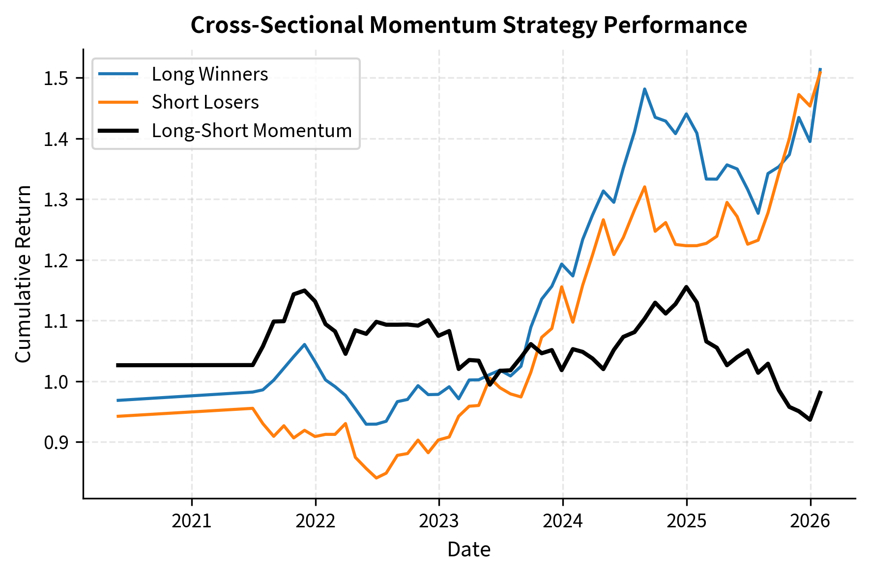
The performance metrics quantify the momentum premium captured by the strategy. A high Sharpe ratio and positive average monthly returns confirm the efficacy of buying winners and selling losers. However, the maximum drawdown indicates that the strategy is not risk-free and can suffer significant drawdowns, particularly during market reversals.

Key ParametersLink Copied

The key parameters for the Cross-Sectional Momentum strategy are:

Formation Period ( $J$ ): The lookback window for ranking stocks (e.g., 12 months).
Holding Period ( $K$ ): The duration positions are held (e.g., 1 month).
Skip Period: The lag between formation and holding periods (e.g., 1 month) to avoid short-term reversals.
Portfolio Size: The number or percentage of stocks in the long and short legs (e.g., top/bottom decile).

Historical Evidence and the Momentum PremiumLink Copied

The momentum anomaly has been documented extensively across markets, time periods, and asset classes:

Equity markets: Momentum profits have been found in the US (Jegadeesh and Titman, 1993), international developed markets (Rouwenhorst, 1998), and emerging markets (Rouwenhorst, 1999)
Asset classes: Momentum works in currencies (Menkhoff et al., 2012), commodities (Miffre and Rallis, 2007), and government bonds (Moskowitz et al., 2012)
Historical depth: Geczy and Samonov (2016) documented momentum profits in US equities back to 1801

The persistence of momentum across such diverse settings suggests it reflects fundamental aspects of how information gets incorporated into prices rather than data mining or statistical artifacts.

The Momentum Factor (UMD)

In factor models discussed in Part IV, momentum is captured by the UMD (Up Minus Down) factor, representing the return of recent winners minus recent losers. This factor has historically earned a premium comparable to the value and size factors, making it a crucial component of multi-factor equity strategies.

Behavioral and Structural Sources of MomentumLink Copied

The profitability of momentum strategies requires explanation. If markets are efficient, past returns should not predict future returns. Several theories attempt to explain why momentum persists.

Investor UnderreactionLink Copied

The most widely cited explanation involves gradual information diffusion and investor underreaction. When new information arrives, prices do not immediately adjust to reflect its full implications. Instead, the adjustment occurs gradually as more investors learn about and trade on the information.

Underreaction can arise from several psychological biases:

Conservatism bias: Investors are slow to update their beliefs when confronted with new evidence, anchoring too heavily on prior views
Inattention: Not all investors monitor all securities continuously; information spreads gradually through the investor population
Disposition effect: Investors are reluctant to realize losses and eager to realize gains, creating selling pressure on winners and buying pressure on losers that slows price adjustment

The underreaction hypothesis predicts that prices will continue to drift in the direction of initial news as the market gradually incorporates information, generating momentum in returns.

Overreaction and Positive FeedbackLink Copied

An alternative view suggests that momentum itself creates more momentum through positive feedback mechanisms:

Herding: Investors observe others buying and interpret this as a signal of private information, leading them to buy as well
Overconfidence: Traders who profit from momentum trades may become overconfident and increase their positions, pushing prices further
Feedback trading: Technical traders and trend followers explicitly buy rising assets and sell falling assets, amplifying price movements

Under this view, momentum returns eventually reverse as prices overshoot fundamental value. This is consistent with long-horizon return reversals documented at 3- to 5-year horizons.

Risk-Based ExplanationsLink Copied

A third perspective argues that momentum returns represent compensation for bearing systematic risk. Possible risk sources include:

Crash risk: Momentum strategies are exposed to sudden, severe losses when trends reverse abruptly
Liquidity risk: Momentum portfolios may load on less liquid securities that require compensation
Macroeconomic risk: Winners and losers may have different exposures to business cycle risk

The debate between behavioral and risk-based explanations remains unresolved, and the truth likely involves elements of both.

Out[20]:

Visualization

Stylized illustration of momentum dynamics: initial underreaction to news creates momentum as prices gradually adjust, potentially followed by overreaction and eventual reversal. The horizontal dashed line represents the fundamental value implied by the news.

Visualizing Momentum DecayLink Copied

We can examine how momentum profits vary with the formation period lookback, revealing the typical pattern of return persistence and eventual reversal:

In[21]:

Code

# Calculate average returns for different formation periods
formation_periods = [1, 3, 6, 12, 24, 36, 48, 60]  # in months
average_spreads = []

for period in formation_periods:
    lookback = period * 21  # Convert to trading days

    if lookback >= len(stock_prices) - 252:
        average_spreads.append(np.nan)
        continue

    # Calculate momentum for this lookback
    mom_scores = stock_prices.pct_change(lookback)

    # Average monthly spread
    spreads = []
    for date in rebalance_dates[max(1, period + 1) : -1]:
        try:
            scores = mom_scores.loc[date].dropna()
            if len(scores) >= 10:
                sorted_scores = scores.sort_values(ascending=False)
                winner_ret = sorted_scores.head(5).mean()
                loser_ret = sorted_scores.tail(5).mean()
                spreads.append(winner_ret - loser_ret)
        except (KeyError, IndexError):
            pass

    average_spreads.append(np.mean(spreads) if spreads else np.nan)

lookback_analysis = pd.DataFrame(
    {
        "Formation Period (months)": formation_periods,
        "Average Winner-Loser Spread": average_spreads,
    }
)

# Calculate average returns for different formation periods
formation_periods = [1, 3, 6, 12, 24, 36, 48, 60]  # in months
average_spreads = []

for period in formation_periods:
    lookback = period * 21  # Convert to trading days

    if lookback >= len(stock_prices) - 252:
        average_spreads.append(np.nan)
        continue

    # Calculate momentum for this lookback
    mom_scores = stock_prices.pct_change(lookback)

    # Average monthly spread
    spreads = []
    for date in rebalance_dates[max(1, period + 1) : -1]:
        try:
            scores = mom_scores.loc[date].dropna()
            if len(scores) >= 10:
                sorted_scores = scores.sort_values(ascending=False)
                winner_ret = sorted_scores.head(5).mean()
                loser_ret = sorted_scores.tail(5).mean()
                spreads.append(winner_ret - loser_ret)
        except (KeyError, IndexError):
            pass

    average_spreads.append(np.mean(spreads) if spreads else np.nan)

lookback_analysis = pd.DataFrame(
    {
        "Formation Period (months)": formation_periods,
        "Average Winner-Loser Spread": average_spreads,
    }
)

Out[22]:

Visualization

Bar chart showing average winner-minus-loser spread for different formation period lengths. — Momentum profit decay across different formation period lookbacks. Intermediate horizons (6-12 months) typically show the strongest momentum, while very long lookbacks exhibit mean reversion.

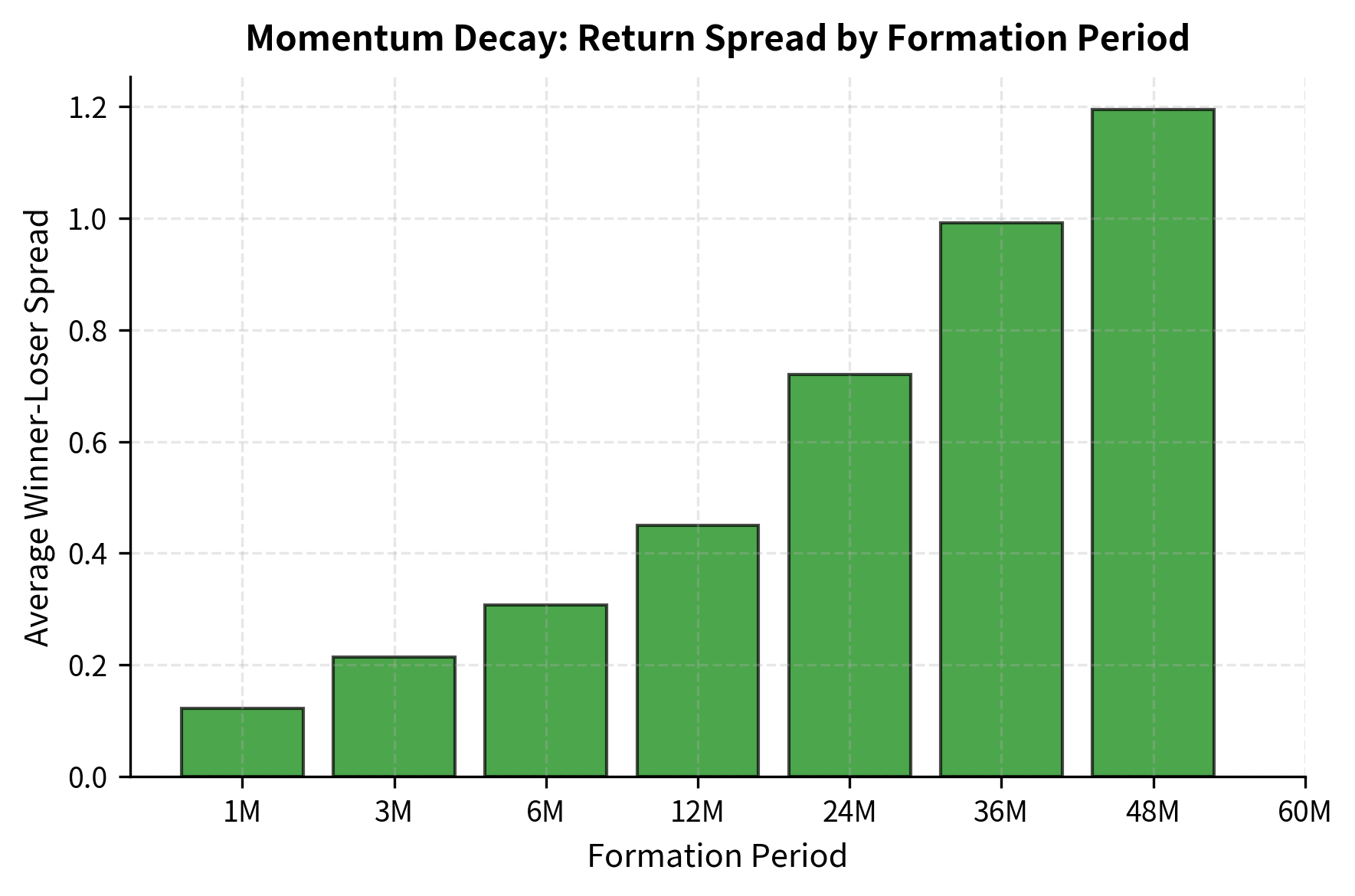
This pattern of intermediate-horizon momentum followed by long-horizon reversal is consistent with both the initial underreaction and subsequent overreaction hypotheses.

Momentum Risks and CrashesLink Copied

Despite its historical profitability, momentum is subject to significant risks that can produce catastrophic losses. Understanding these risks is essential for you.

Momentum CrashesLink Copied

The most severe risk facing momentum strategies is the momentum crash: sudden, violent reversals that produce large losses in a short time. The most famous example occurred in March-May 2009, when momentum strategies lost over 40% in just two months as previously battered financial stocks surged and prior winners collapsed.

Momentum crashes share common characteristics:

They typically occur after extended market declines when losers are at extreme valuations
They coincide with sharp market reversals (bear market rallies)
They involve a rapid unwind as trend followers simultaneously reverse positions
Losses can exceed years of accumulated profits in weeks

In[23]:

Code

# Simulate momentum crash dynamics
np.random.seed(42)
n_days = 252 * 3
dates = pd.date_range(start="2007-01-01", periods=n_days, freq="B")

# Create stylized market scenario: crash then recovery
market_returns = np.concatenate(
    [
        np.random.normal(0.0005, 0.01, 252),  # Normal year
        np.random.normal(-0.003, 0.03, 200),  # Crash period
        np.random.normal(0.01, 0.04, 60),  # Sharp recovery (momentum crash)
        np.random.normal(0.0004, 0.012, n_days - 512),  # Normalization
    ]
)[:n_days]

# Momentum signal based on past 6-month returns
cumulative_market = pd.Series((1 + market_returns).cumprod(), index=dates)
lookback = 126
momentum_signal = np.sign(
    cumulative_market / cumulative_market.shift(lookback) - 1
)

# Strategy returns
strategy_daily = momentum_signal.shift(1) * pd.Series(
    market_returns, index=dates
)
cumulative_mom = (1 + strategy_daily).cumprod()

# Calculate drawdowns
rolling_max_mom = cumulative_mom.expanding().max()
drawdown_mom = cumulative_mom / rolling_max_mom - 1

# Simulate momentum crash dynamics
np.random.seed(42)
n_days = 252 * 3
dates = pd.date_range(start="2007-01-01", periods=n_days, freq="B")

# Create stylized market scenario: crash then recovery
market_returns = np.concatenate(
    [
        np.random.normal(0.0005, 0.01, 252),  # Normal year
        np.random.normal(-0.003, 0.03, 200),  # Crash period
        np.random.normal(0.01, 0.04, 60),  # Sharp recovery (momentum crash)
        np.random.normal(0.0004, 0.012, n_days - 512),  # Normalization
    ]
)[:n_days]

# Momentum signal based on past 6-month returns
cumulative_market = pd.Series((1 + market_returns).cumprod(), index=dates)
lookback = 126
momentum_signal = np.sign(
    cumulative_market / cumulative_market.shift(lookback) - 1
)

# Strategy returns
strategy_daily = momentum_signal.shift(1) * pd.Series(
    market_returns, index=dates
)
cumulative_mom = (1 + strategy_daily).cumprod()

# Calculate drawdowns
rolling_max_mom = cumulative_mom.expanding().max()
drawdown_mom = cumulative_mom / rolling_max_mom - 1

Out[24]:

Visualization

Line chart comparing market and momentum strategy returns during a crash and recovery scenario. — Stylized momentum crash scenario during a market recovery. The strategy suffers severe losses as previously underperforming assets rebound sharply, reversing the gains accumulated during the initial market decline.

Area chart showing strategy drawdown over time. — Drawdown profile of the momentum strategy. The chart reveals the asymmetric risk of momentum investing, where rapid regime shifts lead to deep drawdowns that erase years of steady profits in a few months.

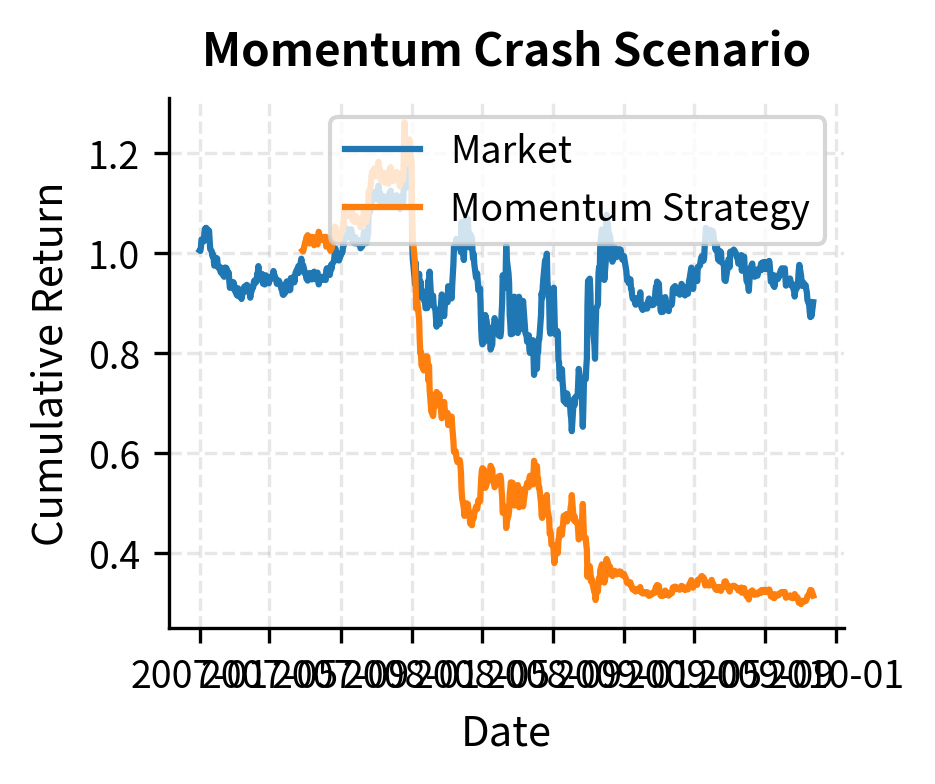
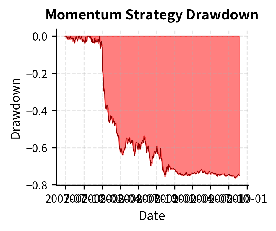
The simulation demonstrates the asymmetry of momentum crashes: gains accumulate gradually over the "normal" period, but the reversal during the recovery phase (when losers outperform winners) wipes out substantial value in a fraction of the time.

Mitigating Momentum Crash RiskLink Copied

Several techniques can reduce, though not eliminate, momentum crash risk:

Volatility scaling: Reduce position sizes when market volatility rises, as crashes often occur in high-volatility regimes
Dynamic hedging: Combine momentum with value or mean reversion to offset crash exposure
Option protection: Purchase put options on momentum portfolios as tail risk insurance
Faster signal adaptation: Use shorter lookback periods that can reverse more quickly
Diversification: Spread momentum across uncorrelated asset classes and markets

In[25]:

Code

# Implement volatility-scaled momentum
vol_lookback = 21
rolling_vol = pd.Series(market_returns, index=dates).rolling(
    vol_lookback
).std() * np.sqrt(252)
vol_target = 0.15

# Scale positions inversely with volatility
vol_scalar = vol_target / rolling_vol
vol_scalar = vol_scalar.clip(upper=3.0, lower=0.25)  # Limit leverage

vol_scaled_strategy = (
    momentum_signal.shift(1)
    * pd.Series(market_returns, index=dates)
    * vol_scalar
)
cumulative_vol_scaled = (1 + vol_scaled_strategy).cumprod()

# Calculate metrics for comparison
unscaled_metrics = calculate_metrics(strategy_daily)
vol_scaled_metrics = calculate_metrics(vol_scaled_strategy)

# Implement volatility-scaled momentum
vol_lookback = 21
rolling_vol = pd.Series(market_returns, index=dates).rolling(
    vol_lookback
).std() * np.sqrt(252)
vol_target = 0.15

# Scale positions inversely with volatility
vol_scalar = vol_target / rolling_vol
vol_scalar = vol_scalar.clip(upper=3.0, lower=0.25)  # Limit leverage

vol_scaled_strategy = (
    momentum_signal.shift(1)
    * pd.Series(market_returns, index=dates)
    * vol_scalar
)
cumulative_vol_scaled = (1 + vol_scaled_strategy).cumprod()

# Calculate metrics for comparison
unscaled_metrics = calculate_metrics(strategy_daily)
vol_scaled_metrics = calculate_metrics(vol_scaled_strategy)

Out[26]:

Visualization

Comparison of unscaled and volatility-scaled momentum strategies. Volatility scaling reduces exposure during high-volatility crash periods, limiting drawdowns while maintaining exposure during calmer trending markets.

Out[27]:

Console

Momentum Strategy: Unscaled vs Volatility-Scaled
=======================================================
Metric                         Unscaled    Vol-Scaled
-------------------------------------------------------
Annualized Return               -37.0%       -10.8%
Annualized Volatility            36.0%        15.4%
Sharpe Ratio                      -1.03         -0.70
Maximum Drawdown                -76.3%       -40.8%

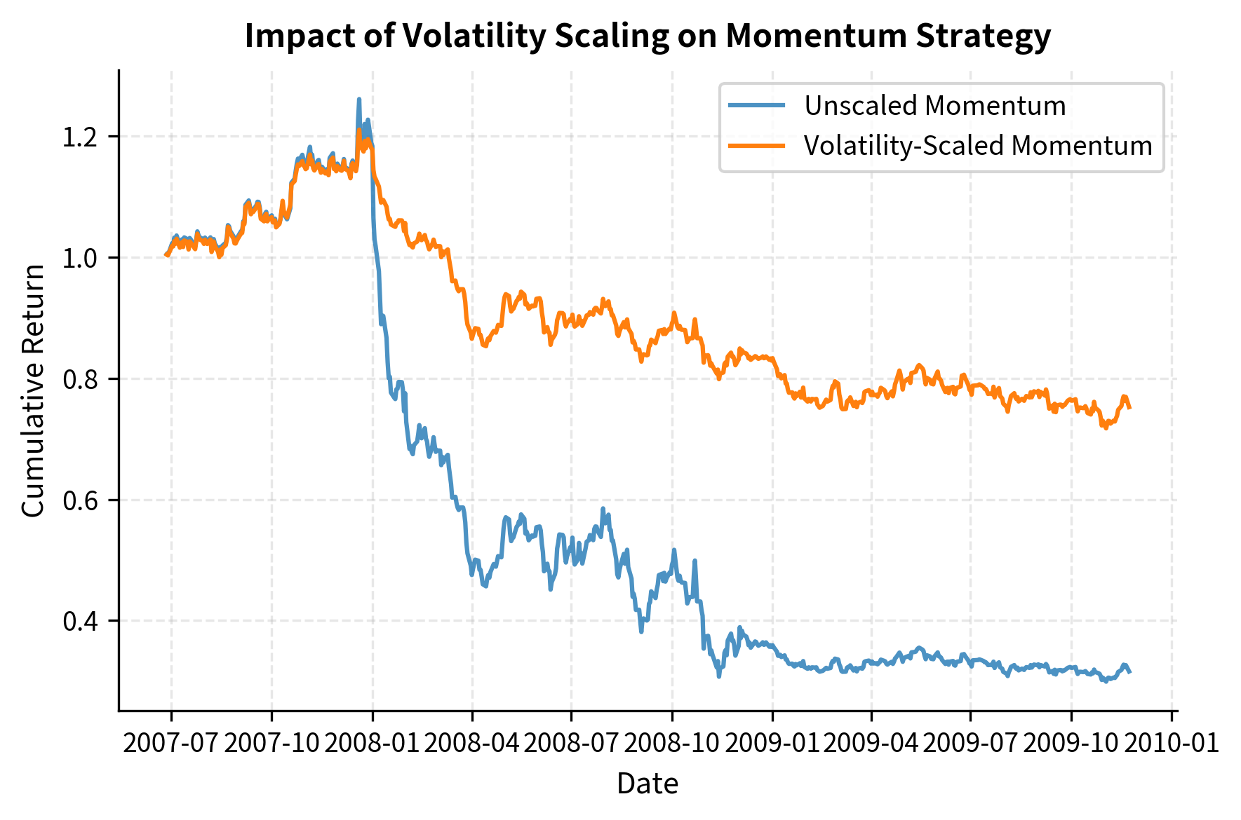
The comparison shows that volatility scaling helps stabilize performance. By reducing exposure when market risk is high, the scaled strategy often suffers a smaller maximum drawdown compared to the unscaled version. Volatility scaling typically improves risk-adjusted returns by reducing exposure during high-volatility crash periods while maintaining exposure during calmer trending periods.

Key ParametersLink Copied

The key parameters for Volatility Scaling are:

Volatility Lookback: Window used to estimate recent market volatility (e.g., 21 days).
Target Volatility: The annualized volatility level the strategy aims to maintain.
Scaling Factor: The multiplier applied to positions, inversely proportional to realized volatility.

Crowding and Capacity ConstraintsLink Copied

As momentum strategies have become more widely adopted, crowding has become a significant concern. When many investors pursue similar momentum trades:

Entry and exit points become more predictable, inviting front-running
Position building takes longer as everyone tries to buy the same stocks
Liquidation events become more severe as positions are unwound simultaneously
Alpha decays as the strategy becomes arbitraged away

You respond to crowding by differentiating your signals (using proprietary data or alternative construction methods), trading more patiently, and monitoring crowding indicators such as short interest concentration or factor positioning surveys.

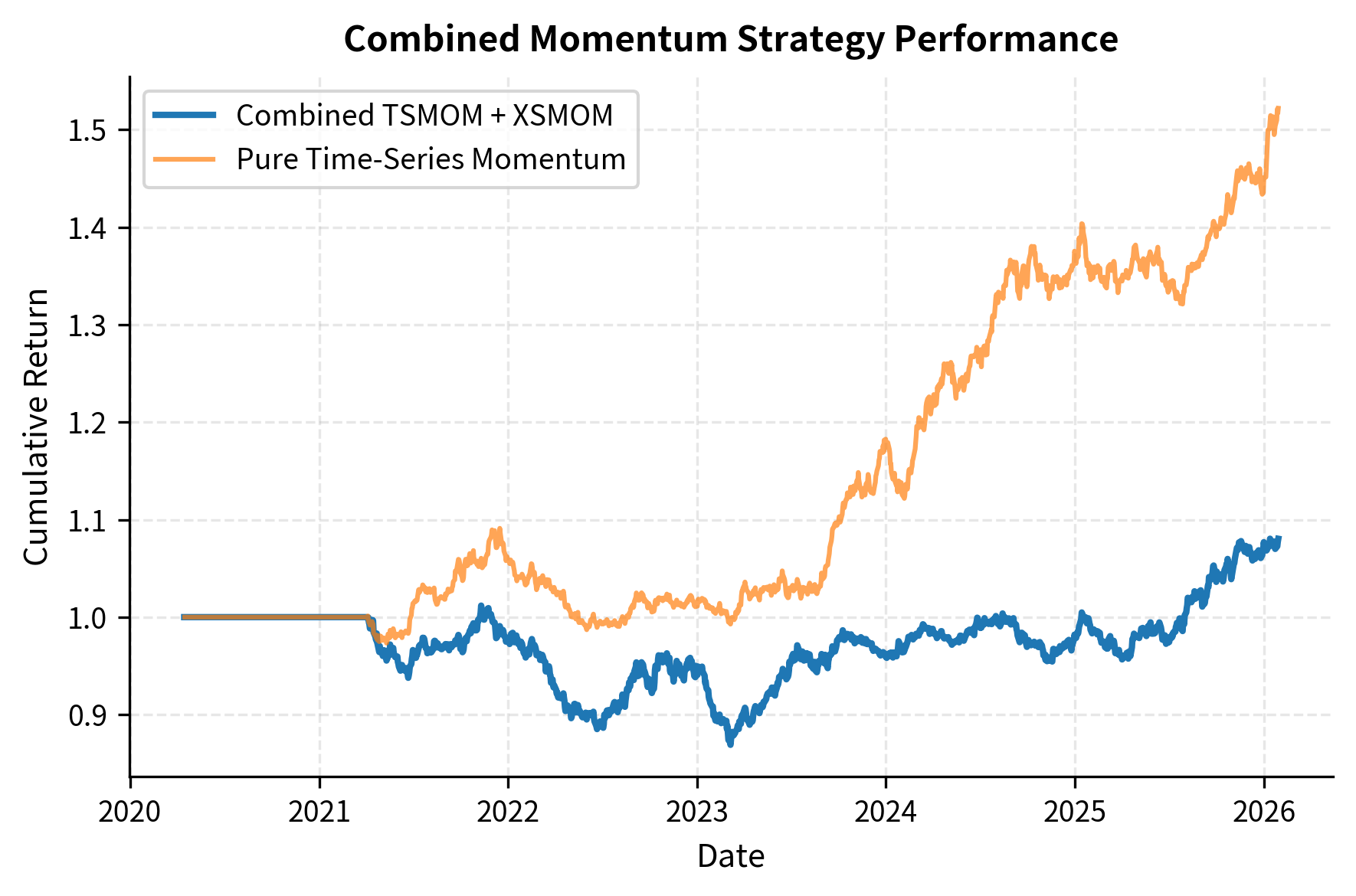
Combining Time-Series and Cross-Sectional MomentumLink Copied

Sophisticated momentum strategies often combine both time-series and cross-sectional signals. Time-series momentum provides absolute direction (should we be long or short the asset class?), while cross-sectional momentum provides relative selection (which assets within the class should we overweight?).

In[28]:

Code

# Combined momentum strategy
def combined_momentum_strategy(prices, ts_lookback=252, xs_lookback=126):
    """
    Combine time-series and cross-sectional momentum.

    Time-series: Go long only when asset has positive momentum
    Cross-sectional: Overweight relative winners, underweight losers
    """
    returns = prices.pct_change()
    n_assets = prices.shape[1]

    # Time-series signals (1 for positive momentum, 0 otherwise)
    ts_signals = pd.DataFrame(index=prices.index, columns=prices.columns)
    for col in prices.columns:
        ts_momentum = prices[col] / prices[col].shift(ts_lookback) - 1
        ts_signals[col] = (ts_momentum > 0).astype(float)

    # Cross-sectional signals (rank-based weights)
    xs_signals = pd.DataFrame(
        index=prices.index, columns=prices.columns, dtype=float
    )
    xs_momentum = prices.pct_change(xs_lookback)

    for date in prices.index[xs_lookback:]:
        scores = xs_momentum.loc[date].dropna()
        if len(scores) > 0:
            ranks = scores.rank()
            # Normalize ranks to weights summing to 1
            xs_signals.loc[date] = (ranks - ranks.mean()) / ranks.sum()

    # Combined signal: time-series filter × cross-sectional weights
    combined_weights = ts_signals * xs_signals

    # Normalize to fully invested when possible
    combined_weights = combined_weights.div(
        combined_weights.abs().sum(axis=1), axis=0
    )
    combined_weights = combined_weights.fillna(0)

    # Portfolio returns
    portfolio_ret = (combined_weights.shift(1) * returns).sum(axis=1)

    return portfolio_ret, combined_weights


combined_returns, combined_weights = combined_momentum_strategy(stock_prices)

# Combined momentum strategy
def combined_momentum_strategy(prices, ts_lookback=252, xs_lookback=126):
    """
    Combine time-series and cross-sectional momentum.

    Time-series: Go long only when asset has positive momentum
    Cross-sectional: Overweight relative winners, underweight losers
    """
    returns = prices.pct_change()
    n_assets = prices.shape[1]

    # Time-series signals (1 for positive momentum, 0 otherwise)
    ts_signals = pd.DataFrame(index=prices.index, columns=prices.columns)
    for col in prices.columns:
        ts_momentum = prices[col] / prices[col].shift(ts_lookback) - 1
        ts_signals[col] = (ts_momentum > 0).astype(float)

    # Cross-sectional signals (rank-based weights)
    xs_signals = pd.DataFrame(
        index=prices.index, columns=prices.columns, dtype=float
    )
    xs_momentum = prices.pct_change(xs_lookback)

    for date in prices.index[xs_lookback:]:
        scores = xs_momentum.loc[date].dropna()
        if len(scores) > 0:
            ranks = scores.rank()
            # Normalize ranks to weights summing to 1
            xs_signals.loc[date] = (ranks - ranks.mean()) / ranks.sum()

    # Combined signal: time-series filter × cross-sectional weights
    combined_weights = ts_signals * xs_signals

    # Normalize to fully invested when possible
    combined_weights = combined_weights.div(
        combined_weights.abs().sum(axis=1), axis=0
    )
    combined_weights = combined_weights.fillna(0)

    # Portfolio returns
    portfolio_ret = (combined_weights.shift(1) * returns).sum(axis=1)

    return portfolio_ret, combined_weights


combined_returns, combined_weights = combined_momentum_strategy(stock_prices)

In[29]:

Code

# Calculate pure strategies for comparison
# Re-calculate TS momentum on the stock universe for fair comparison
ts_lookback = 252
ts_mom_stocks = stock_prices / stock_prices.shift(ts_lookback) - 1
ts_sig_stocks = (ts_mom_stocks > 0).astype(float)
pure_ts_returns = (ts_sig_stocks.shift(1) * stock_returns).mean(axis=1)

# Calculate cumulative returns for plotting
cum_combined = (1 + combined_returns).cumprod()
cum_ts = (1 + pure_ts_returns).cumprod()

# Calculate pure strategies for comparison
# Re-calculate TS momentum on the stock universe for fair comparison
ts_lookback = 252
ts_mom_stocks = stock_prices / stock_prices.shift(ts_lookback) - 1
ts_sig_stocks = (ts_mom_stocks > 0).astype(float)
pure_ts_returns = (ts_sig_stocks.shift(1) * stock_returns).mean(axis=1)

# Calculate cumulative returns for plotting
cum_combined = (1 + combined_returns).cumprod()
cum_ts = (1 + pure_ts_returns).cumprod()

Out[30]:

Visualization

Line chart showing cumulative returns of the combined momentum strategy versus individual approaches. — Performance of the combined momentum strategy. The integrated approach achieves more stable capital growth by filtering the investment universe for absolute momentum before ranking assets relative to peers.

Out[31]:

Visualization

Portfolio weight allocation over time for the combined momentum strategy. The dynamic weights reveal how the absolute momentum filter removes assets during market downturns, concentrating exposure in a rotating set of leading performers.

Limitations and Practical ConsiderationsLink Copied

Momentum strategies, while historically profitable, face several practical challenges that affect real-world implementation.

Transaction costs represent a significant drag on momentum returns. High-turnover strategies that frequently rebalance between winners and losers incur substantial trading costs, particularly when dealing with less liquid securities. Studies that account for realistic transaction costs often find that momentum profits are substantially reduced, especially for strategies using shorter formation and holding periods. You must carefully balance signal freshness against turnover, often implementing partial rebalancing or threshold-based trading rules to reduce costs.

The risk of regime change poses an existential threat to momentum strategies. The anomaly has been documented extensively since the 1990s, attracting substantial capital to momentum-based strategies. As more assets chase the same patterns, the equilibrium expected return should decline. Some researchers argue that momentum profits have already diminished in recent decades, while others contend that the behavioral roots of momentum ensure its persistence. Regardless, you should expect future returns to be lower than historical backtests suggest and should continuously monitor for signs of strategy decay.

Short-selling constraints create asymmetry between the long and short legs of cross-sectional momentum. Shorting stocks involves borrowing costs, potential recalls, and regulatory restrictions that do not affect long positions. Additionally, the short leg often consists of distressed or high-volatility stocks that are difficult and expensive to borrow. Many implementations of momentum focus primarily on the long leg or use long-only momentum-tilted portfolios rather than attempting dollar-neutral long-short strategies.

Finally, momentum strategies interact with other factors in ways that can reduce or enhance returns. Momentum tends to be negatively correlated with value strategies at short horizons, as recent winners often appear expensive while recent losers appear cheap. This creates natural hedging opportunities when combining momentum with value in multi-factor portfolios. We will explore these factor interactions further in the next chapter on Factor Investing and Long/Short Equity.

SummaryLink Copied

Trend following and momentum strategies exploit the tendency of asset prices to exhibit persistence, buying recent winners and selling recent losers. This chapter covered the two main variants of momentum investing and their practical implementation:

Time-series momentum compares an asset's current price to its own history, generating long or short signals based on the direction of recent returns. Moving average crossovers and breakout systems are common implementations. CTA strategies apply time-series momentum across diversified portfolios of futures contracts, benefiting from low correlation to traditional assets and the ability to profit in both rising and falling markets.

Cross-sectional momentum ranks assets relative to their peers, going long the top performers and short the bottom performers. The Jegadeesh-Titman framework established that buying 6- to 12-month winners and selling losers generates significant excess returns across equity markets, time periods, and asset classes.

Behavioral explanations for momentum include investor underreaction to new information, herding behavior, and positive feedback trading. Risk-based explanations suggest momentum returns compensate for crash risk and other systematic exposures. The truth likely involves elements of both.

Momentum crashes represent the strategy's most severe risk, with sudden reversals capable of erasing years of profits in weeks. Volatility scaling, diversification, and dynamic hedging can mitigate but not eliminate this risk. Strategy crowding presents an additional concern as momentum becomes more widely adopted.

The combination of time-series and cross-sectional momentum often produces more robust results than either approach alone. In the next chapter, we will see how momentum combines with other factors such as value, quality, and low volatility in systematic long-short equity strategies.

QuizLink Copied

Ready to test your understanding? Take this quick quiz to reinforce what you've learned about trend following and momentum strategies.

Loading component...

Comments

Back to Quantitative Finance

Previous Chapter

Mean Reversion and Statistical Arbitrage

Next Chapter

Factor Investing and Long/Short Equity

Reference

BIBTEXAcademic

@misc{trendfollowingmomentumtradingstrategyimplementation, author = {Michael Brenndoerfer}, title = {Trend Following & Momentum: Trading Strategy Implementation}, year = {2025}, url = {https://mbrenndoerfer.com/writing/trend-following-momentum-strategies-cta-implementation}, organization = {mbrenndoerfer.com}, note = {Accessed: 2025-01-01} }

APAAcademic

Michael Brenndoerfer (2025). Trend Following & Momentum: Trading Strategy Implementation. Retrieved from https://mbrenndoerfer.com/writing/trend-following-momentum-strategies-cta-implementation

MLAAcademic

Michael Brenndoerfer. "Trend Following & Momentum: Trading Strategy Implementation." 2026. Web. today. <https://mbrenndoerfer.com/writing/trend-following-momentum-strategies-cta-implementation>.

CHICAGOAcademic

Michael Brenndoerfer. "Trend Following & Momentum: Trading Strategy Implementation." Accessed today. https://mbrenndoerfer.com/writing/trend-following-momentum-strategies-cta-implementation.

HARVARDAcademic

Michael Brenndoerfer (2025) 'Trend Following & Momentum: Trading Strategy Implementation'. Available at: https://mbrenndoerfer.com/writing/trend-following-momentum-strategies-cta-implementation (Accessed: today).

SimpleBasic

Michael Brenndoerfer (2025). Trend Following & Momentum: Trading Strategy Implementation. https://mbrenndoerfer.com/writing/trend-following-momentum-strategies-cta-implementation

Direct link:

https://mbrenndoerfer.com/writing/trend-following-momentum-strategies-cta-implementation

About the author: Michael Brenndoerfer

All opinions expressed here are my own and do not reflect the views of my employer.

Michael currently works as an Associate Director of Data Science at EQT Partners in Singapore, leading AI and data initiatives across private capital investments.

With over a decade of experience spanning private equity, management consulting, and software engineering, he specializes in building and scaling analytics capabilities from the ground up. He has published research in leading AI conferences and holds expertise in machine learning, natural language processing, and value creation through data.

View Full Resume Publications Contact Books

Trend Following & Momentum: Trading Strategy Implementation

Trend Following and Momentum StrategiesLink Copied

Time-Series Momentum and Trend FollowingLink Copied

The Mathematical FoundationLink Copied

Implementing Moving Average CrossoversLink Copied

Key ParametersLink Copied

Breakout StrategiesLink Copied

Key ParametersLink Copied

CTA Strategies and Multi-Asset Trend FollowingLink Copied

Key ParametersLink Copied

Cross-Sectional MomentumLink Copied

The Jegadeesh-Titman FrameworkLink Copied

Implementing Cross-Sectional MomentumLink Copied

Key ParametersLink Copied

Historical Evidence and the Momentum PremiumLink Copied

Behavioral and Structural Sources of MomentumLink Copied

Investor UnderreactionLink Copied

Overreaction and Positive FeedbackLink Copied

Risk-Based ExplanationsLink Copied

Visualizing Momentum DecayLink Copied

Momentum Risks and CrashesLink Copied

Momentum CrashesLink Copied

Mitigating Momentum Crash RiskLink Copied

Key ParametersLink Copied

Crowding and Capacity ConstraintsLink Copied

Combining Time-Series and Cross-Sectional MomentumLink Copied

Limitations and Practical ConsiderationsLink Copied

SummaryLink Copied

QuizLink Copied

Comments

Reference

About the author: Michael Brenndoerfer

Related Content

Event-Driven Strategies: Merger Arbitrage to Fixed Income

Volatility Trading Strategies: Delta Hedging, VIX & Arbitrage

Factor Investing: Long-Short Portfolio Construction & Analysis

Stay updated

Comments

About the author: Michael Brenndoerfer

Related Content

Event-Driven Strategies: Merger Arbitrage to Fixed Income

Volatility Trading Strategies: Delta Hedging, VIX & Arbitrage

Factor Investing: Long-Short Portfolio Construction & Analysis

Stay updated