

Master mean reversion trading with cointegration tests, pairs trading, and factor-neutral statistical arbitrage portfolios. Includes regime risk management.
Choose your expertise level to adjust how many terms are explained. Beginners see more tooltips, experts see fewer to maintain reading flow. Hover over underlined terms for instant definitions.
Mean Reversion and Statistical Arbitrage
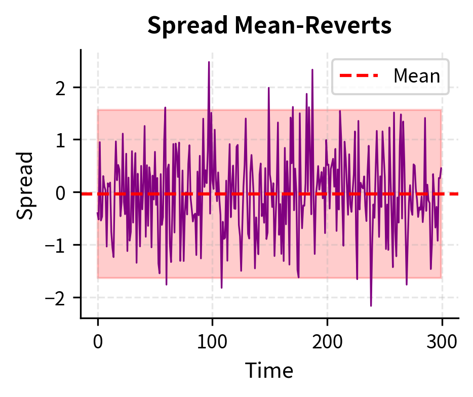
Mean reversion is one of the most intuitive and enduring concepts in quantitative finance. The idea is simple: when prices or spreads deviate significantly from their historical norms, they tend to drift back toward those norms over time. This behavior creates opportunities for traders who can systematically identify and exploit these temporary dislocations.
Unlike trend following strategies that profit from persistent price movements, mean reversion strategies bet against extremes. When a spread between two related securities widens beyond historical bounds, mean reversion traders go long the underperformer and short the outperformer, expecting convergence. When an asset's price falls far below its fair value, they buy expecting recovery.
Statistical arbitrage, often called "stat arb," is the large-scale application of mean reversion principles. Rather than betting on individual pairs, stat arb strategies construct diversified portfolios of many small mean-reverting bets, using statistical models to identify mispricings and manage risk. This approach transformed from a niche strategy at a few quantitative hedge funds in the 1980s into a dominant force in equity markets, with stat arb firms accounting for a significant share of daily trading volume.
This chapter develops the theoretical foundations of mean reversion, builds practical implementations of pairs trading and statistical arbitrage, and examines the risks that have caused even the most sophisticated stat arb strategies to experience dramatic drawdowns.
The Economics of Mean Reversion
Mean reversion arises from several economic mechanisms, each operating on different time scales and asset classes. Understanding these underlying forces is essential because they determine when mean reversion is likely to persist and when it might fail. A trading strategy built on mean reversion is ultimately a bet that certain economic forces will continue to operate, so identifying the source of the reversion informs both strategy design and risk management.
Fundamental Value Anchoring
The most robust form of mean reversion occurs when prices are anchored to fundamental values. This anchoring creates a gravitational pull that prevents prices from drifting too far from intrinsic worth, regardless of short-term market sentiment or technical pressures. Consider a closed-end fund that trades at a discount to its net asset value (NAV). Arbitrageurs can buy the fund, redeem shares at NAV, and pocket the difference. This arbitrage pressure pushes the discount toward zero. While frictions prevent perfect convergence, the discount tends to oscillate around a stable level rather than drifting indefinitely. The key insight here is that the arbitrage mechanism provides a concrete economic force that literally pulls prices back toward fundamental value.
Mean reversion is the tendency of a variable to move toward its long-run average value over time. In finance, this applies to prices, spreads, volatility, and other quantities that exhibit stable long-term behavior despite short-term fluctuations.
Interest rates provide another example where fundamental anchoring creates mean reversion. As we discussed in the chapters on interest rate models, short rates exhibit mean reversion because central banks target rates toward policy objectives, and economic forces create natural equilibrium levels. When rates fall too low, economic activity accelerates and inflationary pressures eventually push rates higher. When rates rise too high, economic activity slows and deflationary pressures eventually pull rates lower. The Vasicek and CIR models we covered in Part III explicitly incorporate mean reversion through parameters that pull rates back toward long-run means, providing a mathematical formalization of these economic intuitions.
Behavioral and Microstructure Effects
Mean reversion also emerges from behavioral biases and market microstructure, representing a second category of economic forces that create trading opportunities. When investors overreact to news, pushing prices beyond fundamental values, subsequent correction creates mean reversion. This overreaction-correction cycle reflects well-documented psychological biases: investors tend to extrapolate recent trends too aggressively and anchor insufficiently to fundamental valuations. The correction phase occurs as cooler heads prevail, as new investors recognize the mispricing, or simply as the emotional intensity of the initial reaction fades.
Similarly, when large orders temporarily push prices away from equilibrium, the price impact decays as the market absorbs the trade. This microstructure-driven mean reversion occurs because the temporary price pressure reflects the mechanical effect of order flow imbalance rather than any change in fundamental value. Once the large order completes execution, the imbalance disappears and prices drift back toward fair value.
These effects operate on shorter time scales and are particularly relevant for high-frequency strategies. The mean reversion in bid-ask bounce, where prices oscillate between bid and ask prices, is exploited by market makers, a topic we'll explore in a later chapter.
Relative Value Relationships
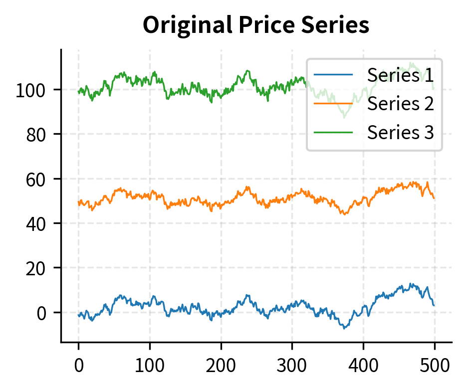
The most important source of mean reversion for statistical arbitrage comes from relative value relationships between securities. When two stocks share common economic exposures, perhaps they're competitors in the same industry, or their earnings depend on the same commodity price, their prices should move together over time. The logic is straightforward: if two companies face similar economic forces, their valuations should change in similar ways. Temporary divergences create trading opportunities because the divergence implies that at least one security is mispriced relative to the other.
These relationships can be formalized through the concept of cointegration, which we'll develop rigorously later in this chapter. Cointegration provides the mathematical framework for identifying securities whose prices are tied together in the long run, even though they may wander apart in the short run.
Testing for Mean Reversion
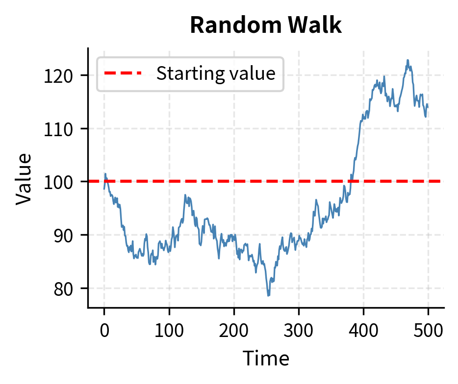
Before trading a mean reversion strategy, you must verify that mean reversion actually exists in your target series. This verification step is essential. A random walk has no mean reversion: past deviations provide no information about future movements. Trading mean reversion on a random walk is a losing proposition because you are betting on convergence that has no statistical tendency to occur.
The distinction between a mean-reverting process and a random walk is subtle but crucial. Both exhibit random fluctuations, and both can appear to drift away from their starting point over short horizons. The difference lies in long-term behavior: a mean-reverting process has a "gravitational center" that pulls it back toward equilibrium, while a random walk has no such anchor and can drift arbitrarily far from any reference point.
The Ornstein-Uhlenbeck Process
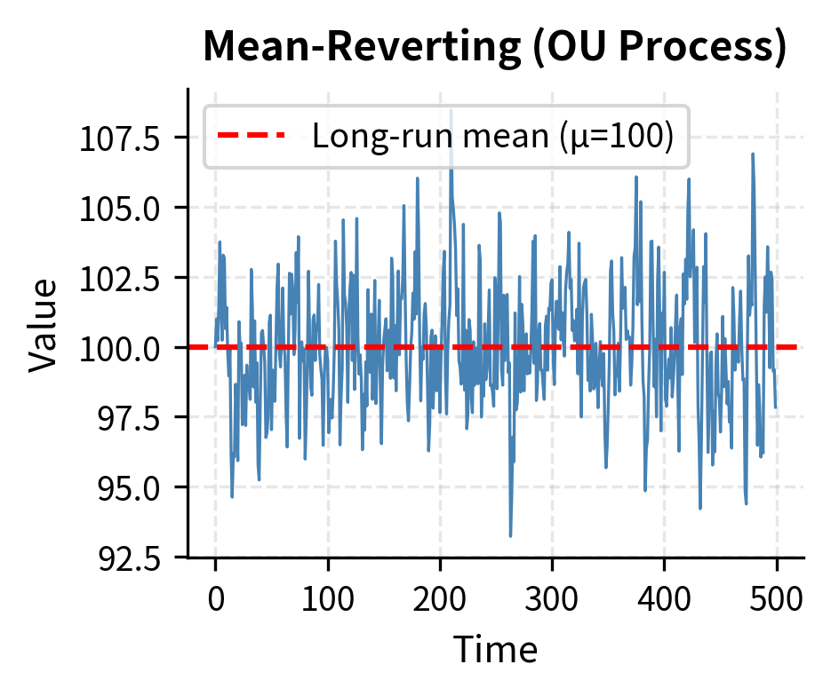
The canonical model for a mean-reverting process is the Ornstein-Uhlenbeck (OU) process. This stochastic differential equation captures the essential dynamics of mean reversion in continuous time, providing a mathematically tractable framework for analysis and parameter estimation. The OU process is defined by:
where:
- : change in the process value
- : value of the process at time
- : speed of mean reversion (higher values mean faster reversion)
- : long-run mean level
- : small time increment
- : volatility of the process
- : standard Brownian motion increment
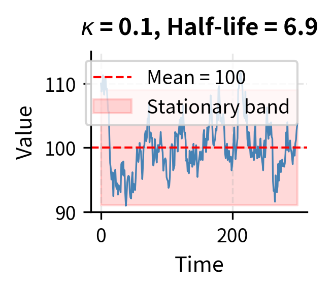
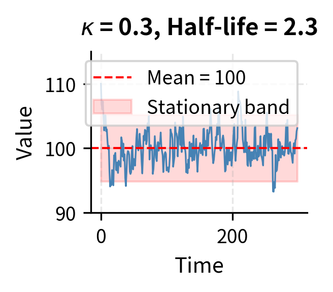
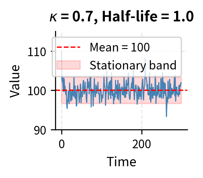
The intuition behind this equation becomes clear when we examine its two components. The first term, , represents the deterministic drift that creates mean reversion. When , the quantity is negative, making the drift term negative, which pushes the process down toward . Conversely, when , the drift is positive, pushing the process up toward . The further the process deviates from , the stronger this restoring force becomes, much like a spring that pulls harder when stretched further.
The parameter controls how quickly this reversion occurs. A high means strong mean reversion, where deviations correct rapidly. A low means weak mean reversion, where the process meanders more before returning to equilibrium. The second term, , represents random shocks that continuously buffet the process, creating the fluctuations around the mean that generate trading opportunities.
The half-life of mean reversion provides a practical measure of how quickly deviations decay. It is the expected time for a deviation to shrink by half:
where:
- : expected time for a deviation to decay by 50%
- : speed of mean reversion
This half-life is crucial for strategy design because it determines the expected holding period for trades. If the half-life is too long relative to your trading horizon, you may not capture the reversion before other factors dominate. For instance, if a spread has a half-life of six months but you need to close positions within weeks due to margin constraints or reporting requirements, you face significant risk that the spread hasn't reverted by the time you must exit. Conversely, if the half-life is very short, perhaps hours or minutes, the strategy may require high-frequency execution capabilities that introduce additional costs and complexity.
The Augmented Dickey-Fuller Test
The Augmented Dickey-Fuller (ADF) test is the workhorse for testing whether a time series is stationary (mean-reverting) or contains a unit root (random walk). The test is constructed around a clever regression specification that directly tests for the presence of mean-reverting behavior. The test estimates the regression:
where:
- : change in the series value at time
- : drift constant
- : coefficient on the time trend
- : coefficient testing for mean reversion (unit root)
- : coefficients on lagged changes capturing serial correlation
- : number of lag terms
- : error term
The key parameter is , which determines the long-run dynamics of the series. The null hypothesis is that , indicating a unit root: the lagged level has no power to predict the current change . Under this null, the series follows a random walk and exhibits no mean reversion.
The alternative hypothesis is , indicating mean reversion. The intuition here is subtle but important. A negative coefficient on the lagged level means that when the series is high (large ), the expected change is negative (pushing the series down). When the series is low (small ), the expected change is positive (pushing the series up). This is precisely the behavior we want: a restoring force that pulls the series back toward its long-run trend.
The lagged changes are included to absorb any serial correlation in the data, ensuring that the test statistic has the correct distribution. A more negative test statistic provides stronger evidence against the null, indicating more convincing mean reversion.
The OU process shows a highly negative test statistic well below the critical values, leading us to reject the null hypothesis of a unit root. The random walk, by contrast, has a test statistic close to zero, and we cannot reject the null. This distinction is fundamental: the OU process is suitable for mean reversion trading, while the random walk is not.
Estimating Mean Reversion Parameters
Once you've established that a series is mean-reverting, you need to estimate the parameters , , and to design trading rules. These parameters have direct practical implications: determines the target level for convergence trades, determines how long you should expect to hold positions, and determines the typical magnitude of fluctuations and hence appropriate position sizing.
The discrete-time analog of the OU process provides the foundation for parameter estimation:
where:
- : value of the process at time
- : speed of mean reversion
- : long-run mean
- : time step size
- : volatility parameter
- : standard normal random variable
This equation shows that the change in the process depends on how far the current value is from the long-run mean, scaled by the mean reversion speed and time step, plus a random shock. Rearranging terms allows us to formulate a linear regression that can be estimated using standard OLS techniques. We begin by expanding the drift term and regrouping:
This algebraic manipulation reveals that the OU process, when discretized, takes the form of a simple autoregressive model. The current value depends linearly on the previous value plus a constant and noise. This matches the form of a simple linear regression:
where:
- : regression intercept
- : regression slope
- : regression residual with variance
The power of this formulation is that simple OLS regression yields estimates of and , from which you can recover the underlying OU parameters. Specifically, solving for from the slope coefficient gives , and substituting into the intercept equation gives . The volatility parameter can be estimated from the standard deviation of the residuals.
The estimated parameters closely match the true values used to generate the series, validating our estimation procedure. The half-life of approximately 1.4 periods tells us that deviations from the mean shrink by half in about 1-2 time steps, indicating quite fast mean reversion.
Pairs Trading: The Classic Implementation
Pairs trading is the simplest and most intuitive application of mean reversion. The strategy involves identifying two securities with prices that move together, then trading the spread when it diverges from its historical norm. The elegance of pairs trading lies in its relative simplicity: rather than predicting absolute price movements, you only need to predict that a divergence will correct.
Finding Suitable Pairs
Good pairs share common economic drivers. The logic is that securities exposed to the same fundamental forces should have prices that co-move over time. When they temporarily diverge, one or both must be mispriced, creating an opportunity for profit when the mispricing corrects. Classic examples include:
- Coca-Cola and PepsiCo (competing soft drink companies)
- Exxon Mobil and Chevron (major oil producers)
- Goldman Sachs and Morgan Stanley (investment banks)
- Different share classes of the same company
- ETFs tracking similar indices
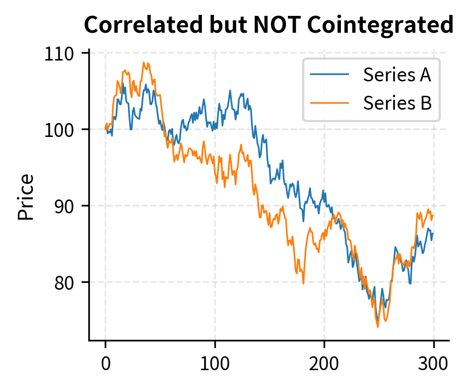
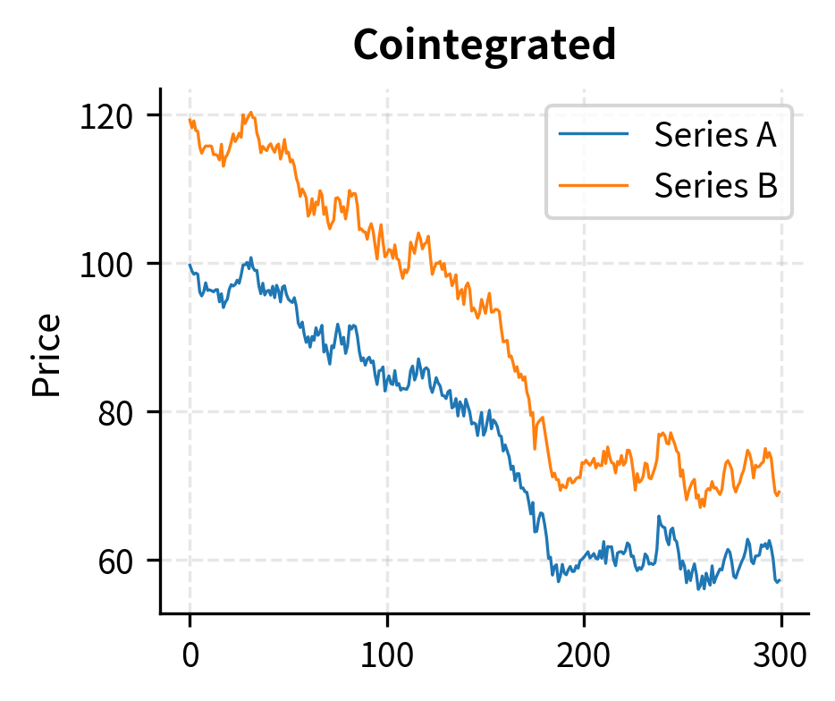
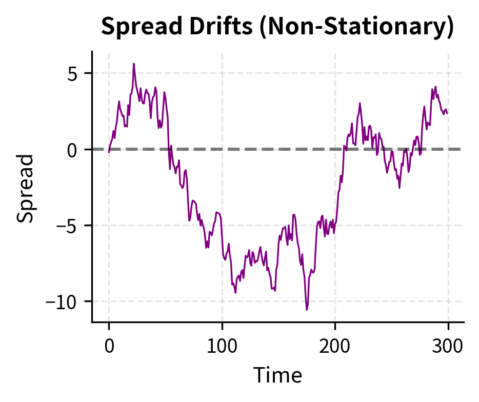
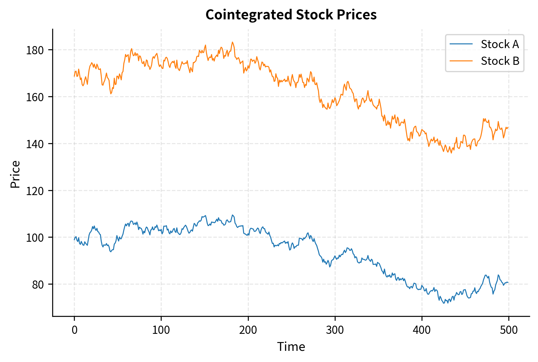
The key requirement is not that the prices be correlated, but that they be cointegrated. This distinction is critical and often misunderstood. Correlation measures how similarly two series move on a percentage basis over short periods. Two highly correlated series can still drift apart indefinitely, making them unsuitable for mean reversion trading. Cointegration, by contrast, captures a much stronger condition: the existence of a stable long-run equilibrium relationship that prevents permanent divergence.
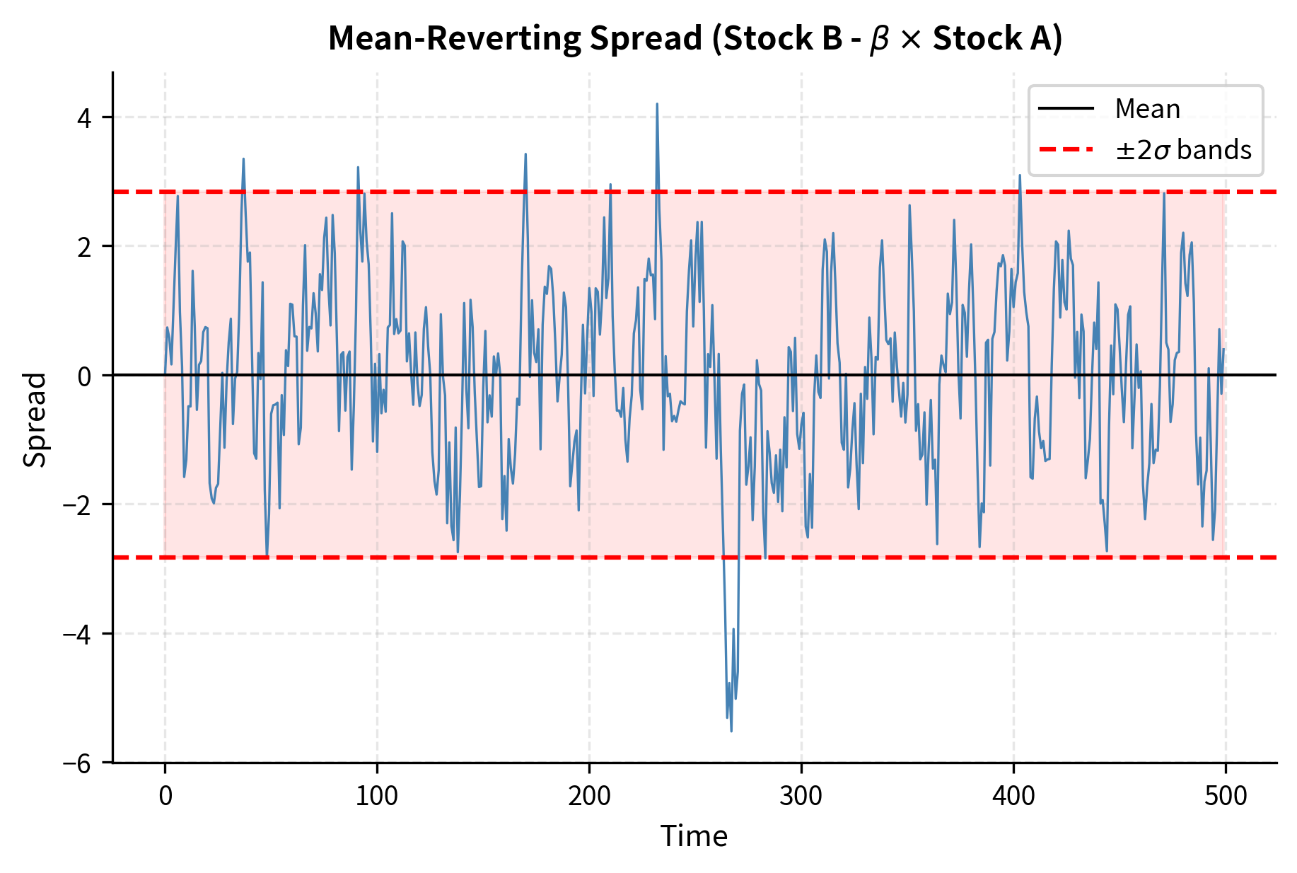
Two series are cointegrated if some linear combination of them is stationary, even though each series individually may be non-stationary. In practical terms, this means you can construct a "spread" from the two prices that mean-reverts, even though neither price individually mean-reverts. This is the foundation of pairs trading.
Two time series and are cointegrated if both are integrated of order 1 (non-stationary with a unit root) but there exists a linear combination that is stationary. The coefficient is called the cointegrating coefficient or hedge ratio.
The Engle-Granger Two-Step Method
The Engle-Granger procedure tests for cointegration and estimates the hedge ratio. The method is elegant in its simplicity: it transforms the problem of testing for cointegration into a standard unit root test on residuals from a regression.
Step 1: Regress one price series on the other:
where:
- : price of the first asset
- : price of the second asset
- : intercept
- : hedge ratio (cointegrating coefficient)
- : residual spread
The regression coefficient tells us how many units of asset we need to hold to hedge one unit of asset . If , for example, then for every share of we buy, we should sell 1.5 shares of to construct a market-neutral spread.
Step 2: Test the residuals for stationarity using the ADF test.
The residuals represent the spread after adjusting for the hedge ratio. If these residuals are stationary, it means the spread cannot drift arbitrarily far from zero; it must revert. This confirms that the series are cointegrated and that is the hedge ratio for constructing the tradeable spread.
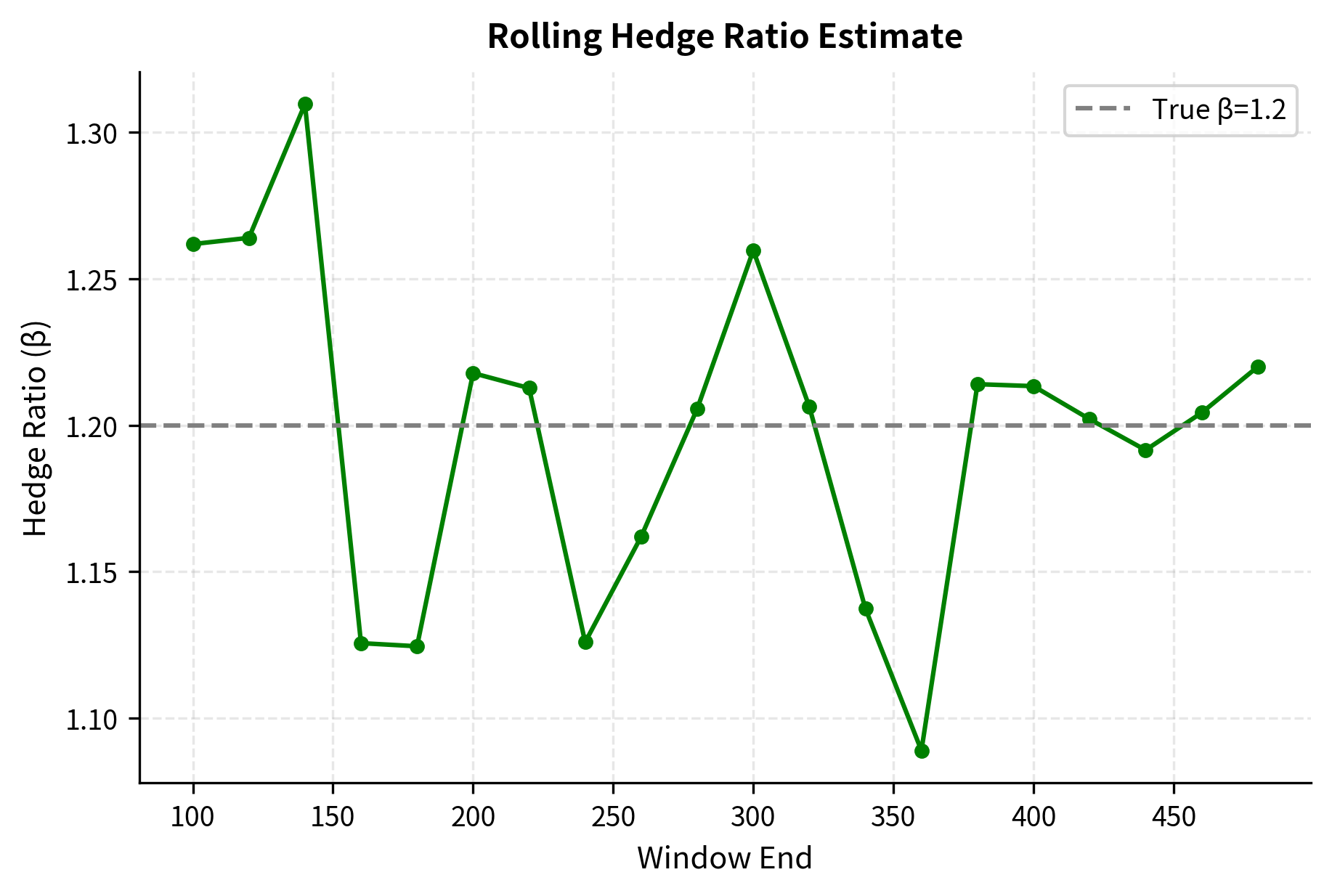
The estimated hedge ratio of approximately 1.20 closely matches the true cointegrating coefficient. The ADF test strongly rejects the null of a unit root in the spread, confirming cointegration.
Trading Rules and Signal Generation
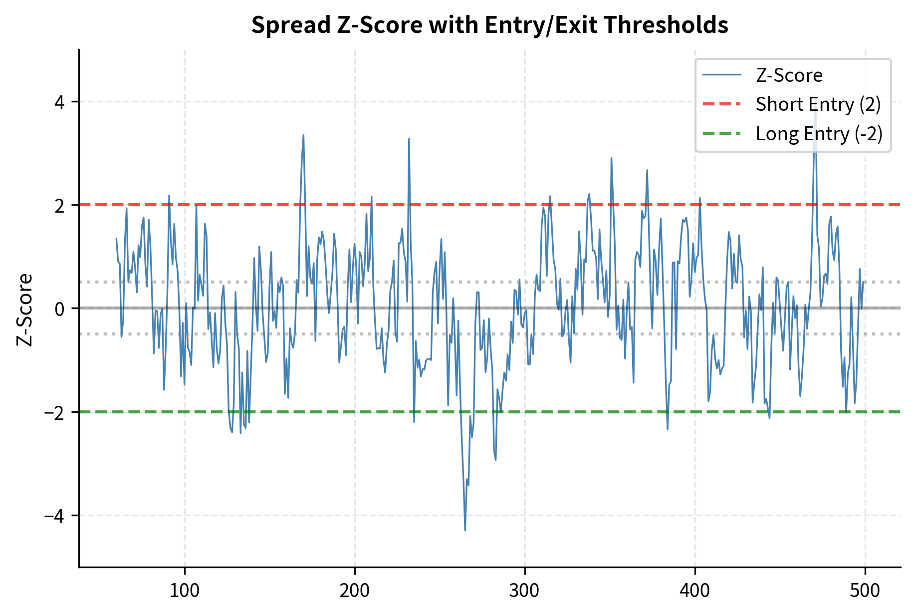
With a cointegrated pair identified, the trading rules follow naturally from the z-score of the spread. The z-score normalizes the spread by its historical mean and standard deviation, transforming it into a standardized measure of how extreme the current deviation is. This normalization serves two purposes: it makes the signal comparable across different pairs with different spread scales, and it provides a natural interpretation in terms of statistical rarity.
where:
- : normalized z-score at time
- : current value of the spread
- : historical mean of the spread
- : historical standard deviation of the spread
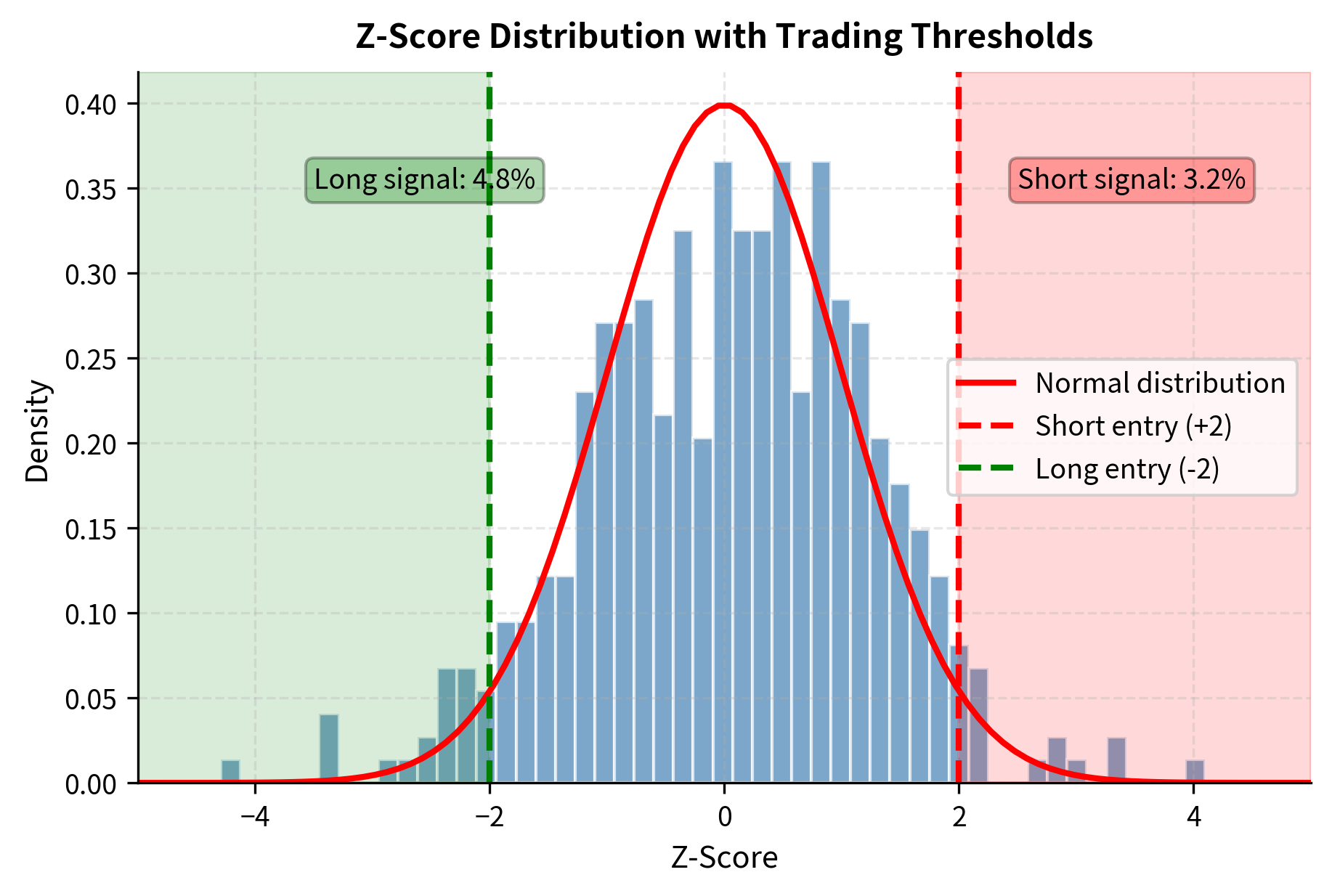
The z-score tells us how many standard deviations the current spread is from its historical mean. A z-score of -2 indicates the spread is two standard deviations below average, an unusually low value that historically has tended to increase. A z-score of +2 indicates an unusually high spread that historically has tended to decrease.
Common entry and exit thresholds are:
- Enter long spread (long Stock B, short Stock A) when
- Enter short spread (short Stock B, long Stock A) when
- Exit position when crosses back to zero or a small threshold like
- Stop loss if exceeds or
These thresholds balance the tradeoff between signal quality and trading frequency. Higher entry thresholds (like ) generate fewer but higher-conviction signals, while lower thresholds (like ) trade more frequently with smaller expected profits per trade.
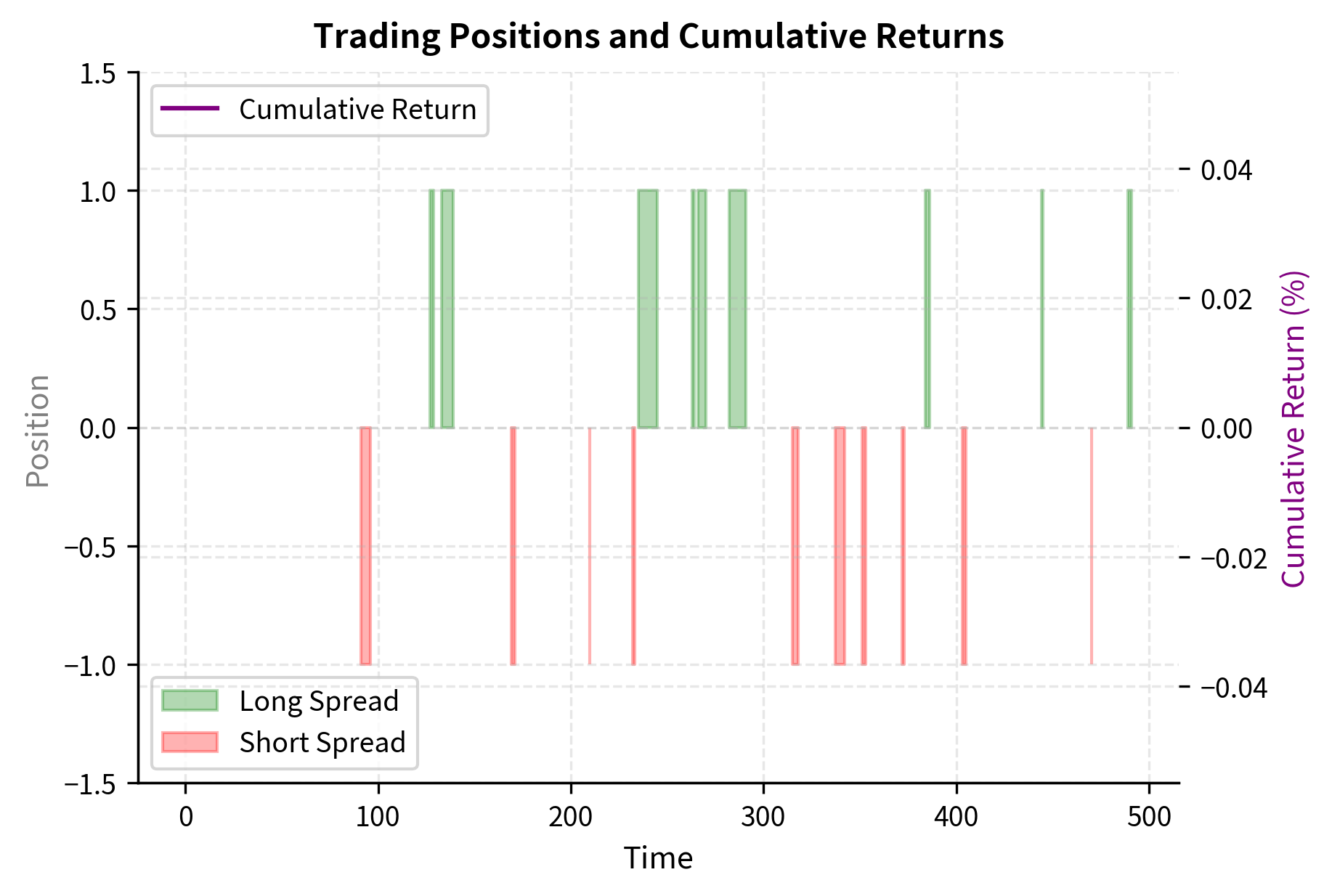
The backtest results indicate a robust strategy, with a Sharpe ratio of 1.93 suggesting attractive risk-adjusted returns. A win rate of 57.5% confirms the predictive power of the mean reversion signal, while the equity curve demonstrates consistent growth despite occasional drawdowns.
Practical Considerations for Pairs Trading
Several practical issues arise when implementing pairs trading:
Rolling vs. expanding windows: We used a 60-day rolling window to estimate the hedge ratio and z-score. This adapts to changing relationships but can introduce noise. Longer windows are more stable but slower to adapt.
Transaction costs: Pairs trading involves frequent rebalancing and trades both legs simultaneously. With 4 legs per round-trip (enter long, enter short, exit long, exit short), transaction costs accumulate quickly.
Margin requirements: Short selling requires margin, and the margin requirement may change based on position size and market conditions.
Execution risk: Both legs must be executed simultaneously to capture the spread. Any delay or partial fill creates unwanted directional exposure.
Key Parameters
The key parameters for the pairs trading strategy are:
- Lookback Window: The historical period used to estimate the hedge ratio and spread statistics. Shorter windows adapt faster but are noisier.
- Entry Threshold: The z-score level (typically ±2.0) that triggers a trade entry.
- Exit Threshold: The z-score level (typically 0 or ±0.5) where the position is closed.
- Stop Loss Threshold: The z-score level (typically ±3.0 to ±4.0) that triggers a forced exit to limit losses.
Statistical Arbitrage: Scaling Beyond Pairs
While pairs trading focuses on individual relationships, statistical arbitrage scales these ideas to portfolios of many small bets. The diversification across many positions is what transforms mean reversion trading from speculation into a more systematic, lower-risk strategy. This scaling is not merely an incremental improvement; it fundamentally changes the risk-return characteristics of mean reversion trading.
From Pairs to Portfolios
A stat arb portfolio might hold 100 or more positions simultaneously, each a small mean reversion bet. The key insight is that if each bet has a modest positive expected return but significant idiosyncratic risk, diversification dramatically improves the Sharpe ratio of the portfolio. This insight follows from basic portfolio theory, but its implications for stat arb are profound.
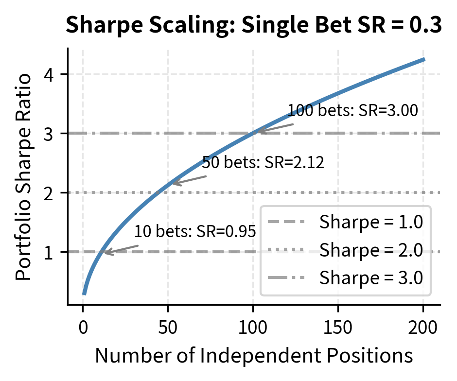
Consider independent mean reversion bets, each with expected return and standard deviation . The portfolio expected return scales linearly with the number of positions, as we simply add up the expected returns: total expected return is . However, the portfolio standard deviation grows more slowly. Because the positions are independent, their risks partially cancel, and the portfolio standard deviation is only (assuming independence). The portfolio Sharpe ratio therefore scales as the square root of the number of positions:
where:
- : Sharpe ratio of the portfolio
- : number of independent positions
- : expected return of each position
- : volatility of each position
- : Sharpe ratio of an individual bet
This scaling is the fundamental appeal of statistical arbitrage. Even if individual bets have modest Sharpe ratios, aggregating many uncorrelated bets can produce impressive risk-adjusted returns. A single mean reversion trade with a Sharpe ratio of 0.3 is hardly exciting, but a portfolio of 100 such independent trades would have a Sharpe ratio of 3.0, which is exceptional by any standard. Of course, in practice the positions are never perfectly independent, so the actual diversification benefit is smaller, but the principle remains powerful.
Factor-Based Statistical Arbitrage
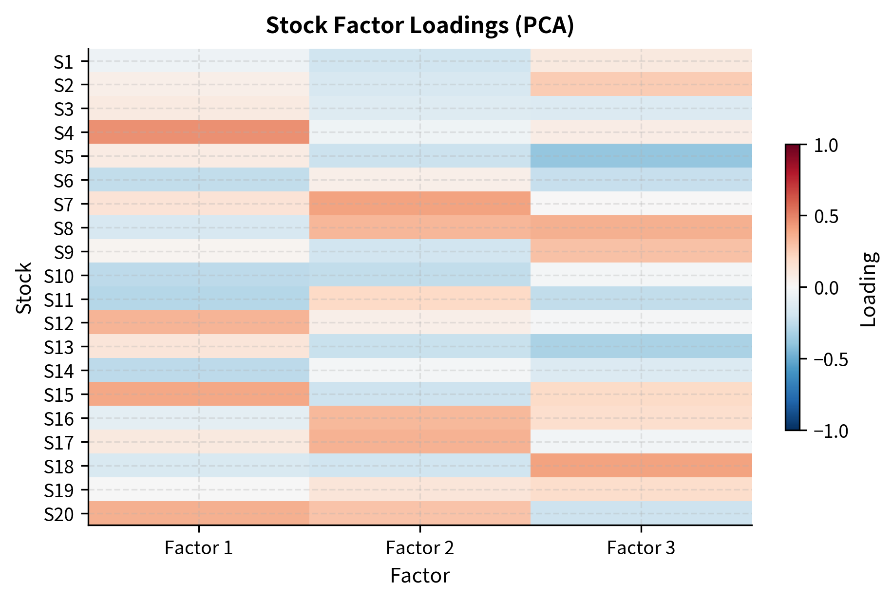
Modern stat arb strategies typically use factor models to construct portfolios. Building on the factor model framework from Part IV, we decompose returns as:
where:
- : return of stock
- : stock-specific expected return (the trading signal)
- : returns of common factors (market, sector, style)
- : number of common factors
- : exposure of stock to factor
- : idiosyncratic (residual) return
This decomposition separates stock returns into two components: the part driven by common factors (market movements, sector rotations, style tilts) and the part that is unique to each stock. The stat arb strategy focuses on capturing the component while hedging out factor exposures. A dollar-neutral, beta-neutral portfolio with many long and short positions isolates idiosyncratic returns from factor movements.
This approach makes sense. Factor movements are notoriously difficult to predict, and betting on them exposes the portfolio to large, correlated risks. By constructing a portfolio that has zero exposure to common factors, we eliminate this source of risk entirely. What remains is idiosyncratic risk, which is diversifiable: with enough positions, the idiosyncratic risks cancel out, leaving only the alpha signal.
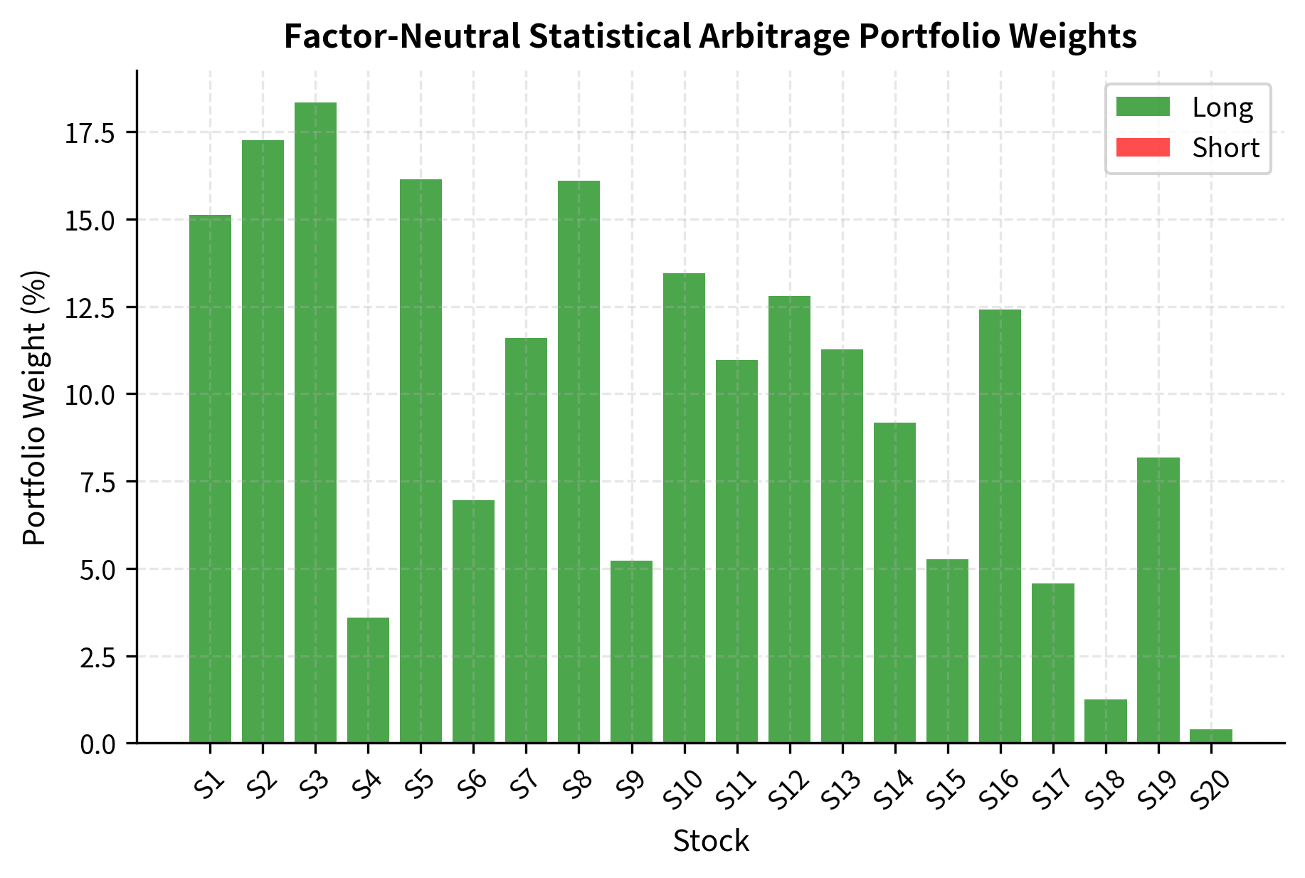
The constructed portfolio achieves the desired properties: the sum of weights is effectively zero (dollar neutrality), and exposure to the three common factors is negligible. This confirms that the portfolio isolates idiosyncratic risk, betting purely on the convergence of residuals.
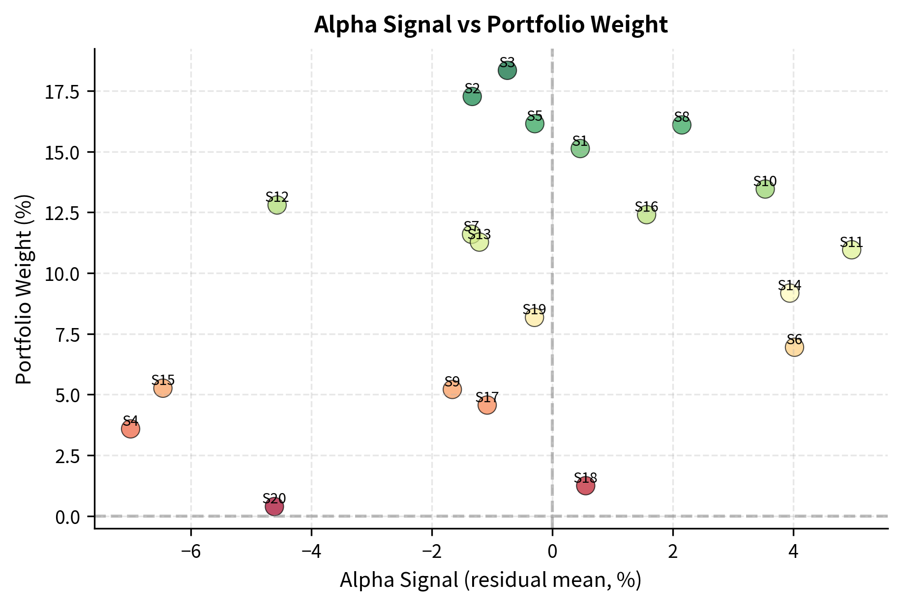
Mean Reversion in the Residual Space
The factor-neutral construction ensures that portfolio returns come primarily from the convergence of idiosyncratic mispricings. When a stock's residual return is abnormally low (negative alpha signal), the portfolio goes long expecting reversion. When residual return is abnormally high, the portfolio goes short. The underlying assumption is that these idiosyncratic deviations are temporary; they reflect noise, overreaction, or short-term supply-demand imbalances rather than permanent changes in fundamental value.
This approach assumes that idiosyncratic returns mean-revert, meaning that temporary mispricings correct themselves. The economic rationale is similar to pairs trading but operates at the level of individual securities rather than pairs. When a stock underperforms after controlling for all known factors, it suggests the market has temporarily mispriced the stock, and we expect correction. The half-life of this mean reversion is typically on the order of days to weeks for equity stat arb strategies.
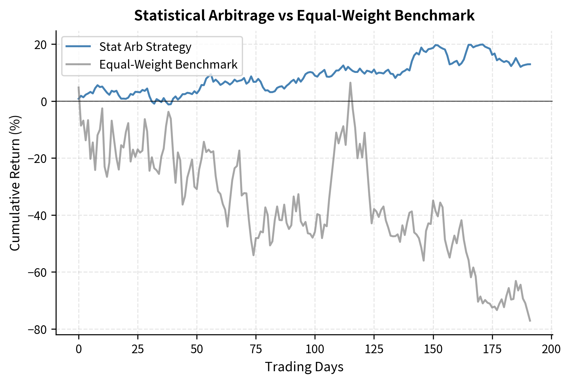
The statistical arbitrage strategy significantly outperforms the benchmark, achieving a higher Sharpe ratio (2.81 vs 0.77) and a lower maximum drawdown. The factor-neutral construction successfully mitigates market risk, resulting in a smoother cumulative return stream compared to the long-only approach.
Key Parameters
The key parameters for statistical arbitrage portfolios are:
- Number of Factors (K): The number of principal components to remove. This determines the granularity of the factor neutrality.
- Lookback Window: The period used to estimate the factor model (PCA) and residual statistics.
- Rebalance Frequency: How often portfolio weights are recalculated. More frequent rebalancing captures faster signals but increases costs.
- Gross Exposure: The total value of long and short positions, typically targeted to a specific leverage level.
The Johansen Test for Multiple Cointegration
When working with more than two securities, the Engle-Granger method becomes cumbersome. The problem is that Engle-Granger requires you to choose one series as the "dependent variable" and can only identify one cointegrating relationship. With three or more securities, there may be multiple independent cointegrating relationships, and the choice of which series to regress on which becomes arbitrary. The Johansen test provides a more general framework for testing cointegration among multiple time series and identifying all cointegrating relationships simultaneously.
Theoretical Framework
The Johansen procedure tests for cointegration in a vector autoregression (VAR) framework using a Vector Error Correction Model (VECM). The VECM representation is particularly elegant because it decomposes price changes into two distinct components: a long-term error correction component that pulls prices back toward equilibrium when they deviate, and short-term autoregressive dynamics that capture momentum and other temporary effects. For a vector of time series , the VECM representation is:
where:
- : vector of price changes at time
- : impact matrix governing long-run error correction
- : vector of price levels at time
- : matrices of coefficients for short-term dynamics
- : lag order of the VAR model
- : vector of error terms
The matrix contains all information about the long-run relationships among the series. Its rank equals the number of cointegrating relationships, providing a complete characterization of the equilibrium structure:
- : No cointegration, all series have unit roots. The series can drift apart without bound.
- : Cointegration exists with cointegrating vectors. There are independent linear combinations of the series that are stationary.
- : All series are stationary. This case is unlikely for price series, which typically have unit roots.
When , the matrix can be decomposed as , where is an matrix whose columns are the cointegrating vectors, and is an matrix of adjustment coefficients that determines how quickly each series responds to deviations from equilibrium.
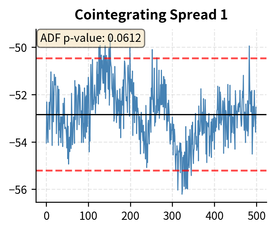
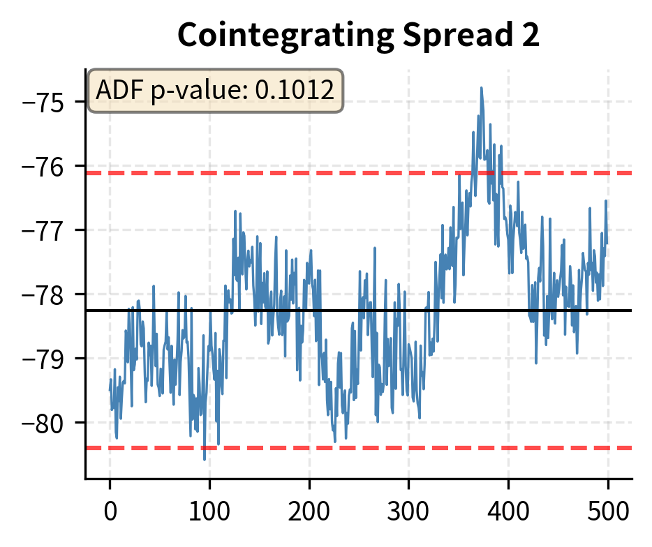
The results show that the trace statistic exceeds the critical values for and , but not for . This implies the existence of two cointegrating relationships () among the three assets, consistent with the data generation process where a single common trend drives all three series. With three series and two cointegrating relationships, there is exactly one common stochastic trend, which matches our construction.
The trace statistic tests the null hypothesis against . When the trace statistic exceeds the critical value, we reject the null and conclude there are more than cointegrating relationships. The sequential testing procedure starts with and continues until we fail to reject, thereby determining the number of cointegrating relationships.
Constructing Baskets from Cointegrating Vectors
The cointegrating vectors from the Johansen test define stationary linear combinations of the prices. These become tradeable spreads for stat arb strategies. Each cointegrating vector specifies the weights to use when combining the securities into a spread. For instance, if the first cointegrating vector is , the corresponding spread is computed as . This spread will be stationary even though each individual series is non-stationary.
Regime Changes and Strategy Risks
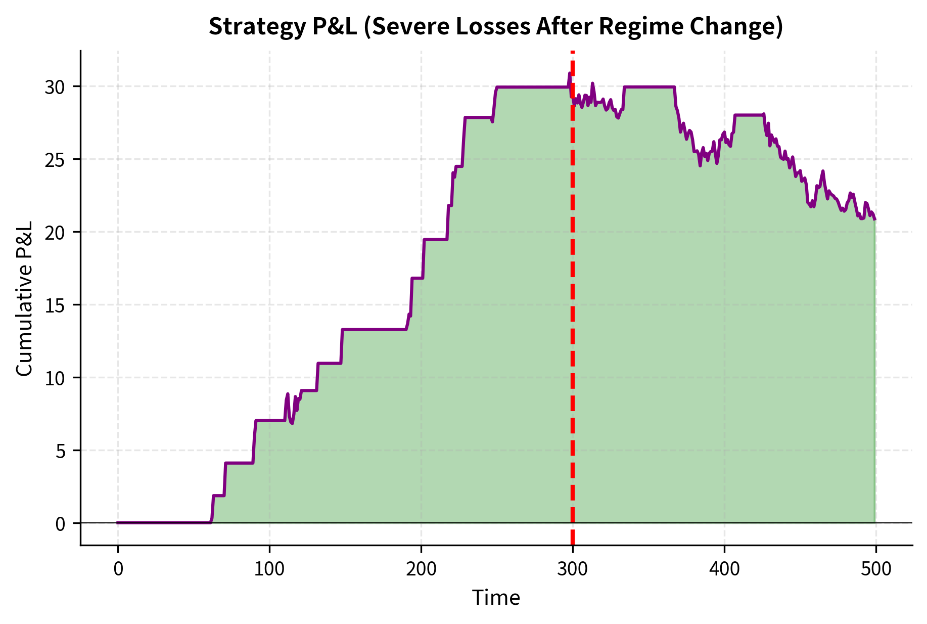
Mean reversion strategies face several risks that can cause significant losses. Understanding these risks is essential for proper strategy design and risk management. The most important insight is that mean reversion strategies implicitly assume the persistence of certain statistical relationships, and these assumptions can fail catastrophically.
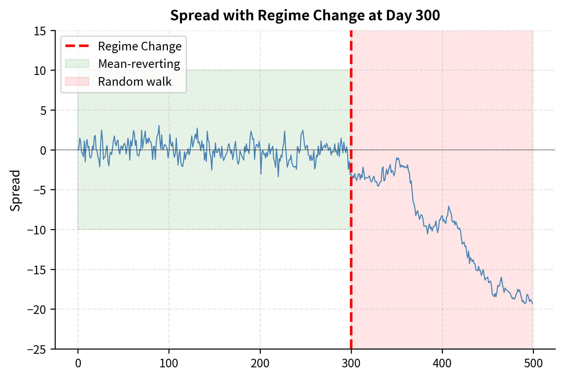
The Danger of Broken Relationships
The most severe risk for mean reversion strategies occurs when assumed relationships permanently break. A spread that has mean-reverted for years can suddenly diverge and never return. This is not merely a statistical tail event; it represents a fundamental change in the economic relationship underlying the spread. This happens when:
- Structural changes: Mergers, acquisitions, spin-offs, or bankruptcy can permanently alter a company's relationship to its peers
- Regulatory changes: New regulations can benefit one company at the expense of another
- Technology disruption: Innovation can invalidate previously stable competitive relationships
- Market structure changes: The delisting of one security, or changes in index composition, can break pairs
When a relationship breaks, the mean reversion strategy continues to bet on convergence that will never occur. As the spread continues to diverge, the strategy accumulates larger and larger losses, and the temptation to "double down" (since the spread is now even more extreme) can lead to ruin.
The August 2007 Quant Meltdown
The most dramatic example of regime risk materializing occurred in August 2007. Many quantitative hedge funds using similar stat arb strategies experienced unprecedented losses during a single week. The mechanism was a classic crowded-trade unwind that exposed the hidden fragility of apparently diversified portfolios. The sequence of events unfolded as follows:
- A major fund faced redemptions or losses in other areas and began liquidating its equity stat arb portfolio.
- This created price pressure on exactly the positions other stat arb funds also held, since the funds were using similar factor models and similar alpha signals.
- Other funds saw their positions move against them and either hit risk limits or faced margin calls.
- The resulting forced liquidation amplified the original moves.
- Spreads that had never diverged so far in history kept diverging further.
What made this particularly devastating:
- The strategies were highly levered
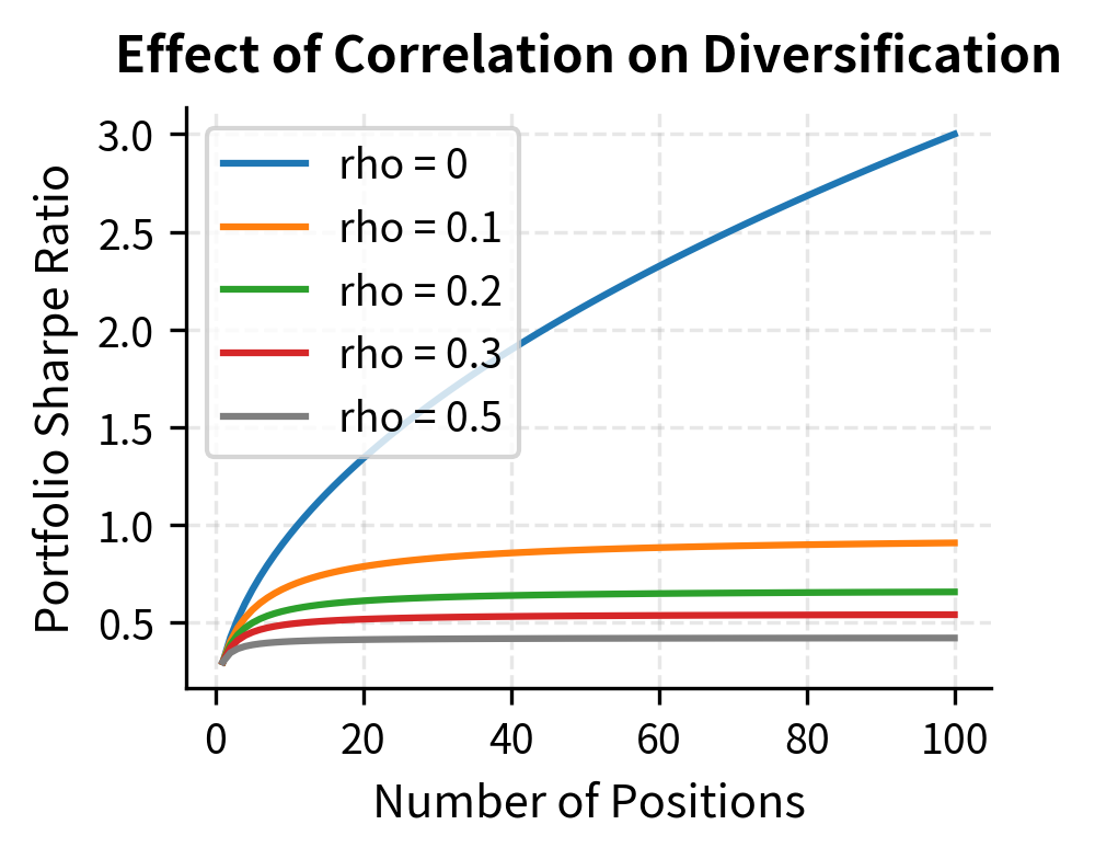
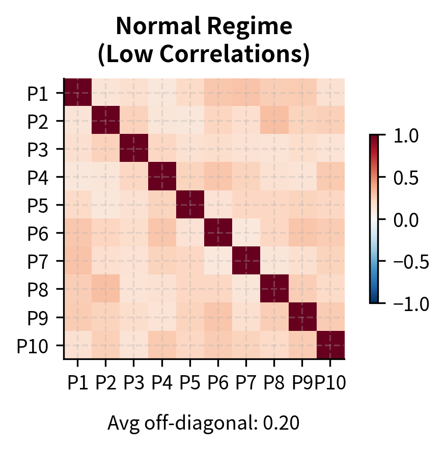
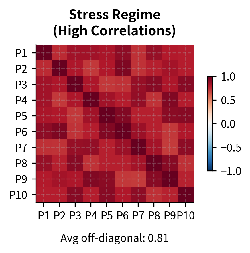
- Diversification across many positions failed, since all positions moved together during the unwind
- The losses exceeded any historical drawdown. The assumption of independence that underlies the diversification benefit proved catastrophically wrong: when everyone rushes for the exit simultaneously, correlations spike to one.
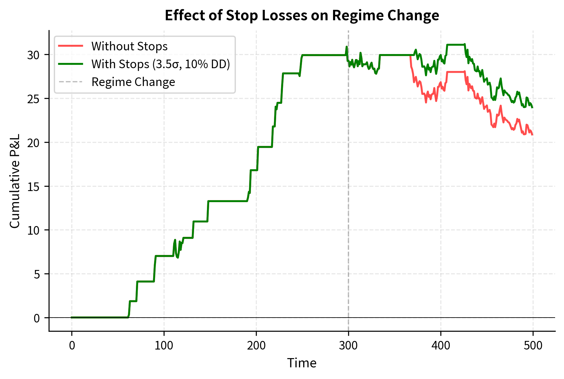
Stop Losses and Position Limits
Protecting against regime risk requires robust risk controls. While no control can eliminate the risk entirely, proper implementation can limit losses to survivable levels.
Position-level stops: Exit any individual pair or basket when the z-score exceeds a threshold (e.g., 4 standard deviations). While this caps individual losses, it also guarantees losses on positions that might have eventually reverted. The tradeoff is between accepting certain small losses now versus risking uncertain large losses later.
Portfolio-level stops: Reduce overall exposure when portfolio drawdown exceeds a threshold. This prevents catastrophic losses but can lock in drawdowns. The key insight is that surviving to trade another day is more important than maximizing expected returns.
Correlation monitoring: Track the correlation of positions. Mean reversion strategies assume idiosyncratic returns, but during stress periods, correlations spike. Reducing positions when correlations rise helps preserve diversification benefits and provides early warning of crowded trade dynamics.
Leverage constraints: The 2007 episode showed that high leverage turns modest percentage losses into existential threats. Conservative leverage ratios (2-3x) leave room to survive extreme events.
Statistical Significance and Overfitting
Another major risk is mistaking random noise for genuine mean reversion. With enough data mining, you can find pairs that appeared to be cointegrated historically but had no true economic relationship. These spurious pairs will fail out of sample because there is no underlying economic force creating the mean reversion; the historical pattern was merely coincidence.
Protecting against overfitting requires:
- Economic rationale: Trade only pairs where you understand why the relationship should hold
- Out-of-sample testing: Validate relationships on data not used in discovery
- Multiple testing correction: When screening many pairs, adjust significance thresholds for the number of tests
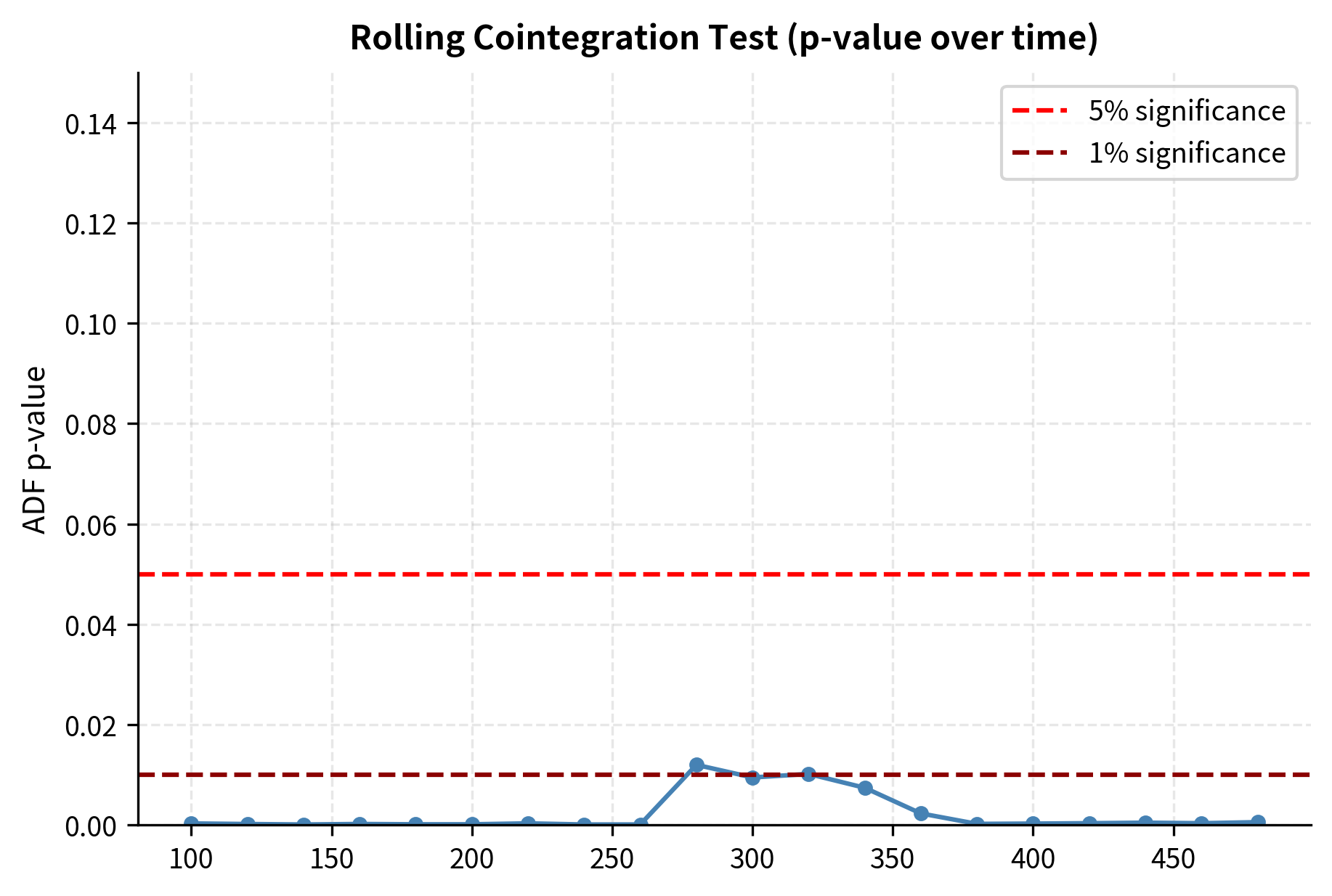
- Rolling cointegration tests: Verify that relationships remain cointegrated over time, not just in the initial training period
Limitations and Impact
This section examines the constraints that limit mean reversion strategies and their broader influence on financial markets.
Limitations
Mean reversion and statistical arbitrage strategies face several inherent limitations that constrain their scalability and profitability.
Capacity constraints represent perhaps the most significant limitation. As stat arb strategies have become more widespread, the mispricings they exploit have shrunk. The trades are by definition temporary dislocations, and more capital chasing the same opportunities compresses returns. Many successful stat arb funds have closed to new investors or returned capital to maintain performance, a stark contrast to strategies that scale more readily.
Model risk is pervasive. Every assumption in a stat arb model can fail: cointegration relationships can break, factor models can miss important exposures, and half-life estimates can be wrong. The models are estimated from historical data that may not represent future market conditions. In particular, the assumption that correlations between positions remain low, the foundation of the diversification benefit, fails precisely when it matters most, during market stress events.
Execution challenges become more severe as strategies operate at higher frequencies or with larger position sizes. The bid-ask spread alone can consume much of the expected profit on mean reversion trades. Market impact pushes prices against you as you trade, reducing returns further. And competition from other quantitative traders means that by the time you identify an opportunity, others may have already acted on it.
Leverage dependency makes stat arb strategies fragile. Because individual mean reversion signals are small, achieving attractive returns requires leverage. This amplifies both returns and risks, and creates vulnerability to margin calls and forced liquidation during drawdowns.
Impact on Markets and Finance
Despite these limitations, statistical arbitrage has fundamentally transformed equity markets. Stat arb strategies act as a powerful force for market efficiency, rapidly correcting mispricings that would have persisted longer in an earlier era. This benefits all market participants through tighter spreads and more accurate prices.
The intellectual framework of stat arb, including using factor models to decompose returns, constructing market-neutral portfolios, and applying statistical tests to trading signals, has influenced far beyond quantitative trading. The factor investing approaches we'll explore in the next chapter owe much to the analytical toolkit developed for stat arb. Risk management practices at traditional asset managers increasingly incorporate the factor-neutral thinking pioneered by stat arb practitioners.
Statistical arbitrage also served as a training ground for quantitative finance talent. Many of the leading figures in quantitative asset management, market making, and fintech began their careers in stat arb. The discipline's rigorous empirical approach of testing every assumption, validating every signal, and measuring every risk has become the standard for quantitative finance more broadly.
The quant meltdown of 2007, while devastating for many funds, also provided invaluable lessons about crowded trades, correlation risk, and the limits of diversification. These lessons informed the development of more robust risk management practices and more conservative leverage policies that characterize the industry today.
Summary
This chapter developed the theory and practice of mean reversion and statistical arbitrage, from the fundamental economic mechanisms that create mean reversion to the practical implementation of trading strategies that exploit it.
Key concepts covered include:
-
Mean reversion fundamentals: The Ornstein-Uhlenbeck process provides a mathematical framework for mean-reverting dynamics, with the mean reversion speed determining how quickly deviations correct.
-
Testing for mean reversion: The Augmented Dickey-Fuller test distinguishes mean-reverting series from random walks, essential for validating trading strategies.
-
Cointegration: Two non-stationary series are cointegrated if a linear combination is stationary. The Engle-Granger and Johansen procedures test for cointegration and estimate hedge ratios.
-
Pairs trading: The classic mean reversion strategy trades the spread between cointegrated securities using z-score signals, going long when the spread is unusually low and short when unusually high.
-
Statistical arbitrage portfolios: Factor-neutral construction using PCA isolates idiosyncratic returns while hedging common factor exposures, enabling diversification across many small mean reversion bets.
-
Regime risk: Relationships can permanently break, causing mean reversion strategies to accumulate losses. Stop losses, position limits, and correlation monitoring help manage this risk.
-
Practical challenges: Transaction costs, execution risk, model instability, and capacity constraints limit strategy profitability.
The next chapter examines trend following and momentum strategies, which take the opposite view from mean reversion. Rather than betting against price movements, momentum strategies bet that recent trends will continue, exploiting a different market inefficiency entirely.
Quiz
Ready to test your understanding? Take this quick quiz to reinforce what you've learned about mean reversion and statistical arbitrage.

Comments