Event-Driven Strategies: Merger Arbitrage to Fixed Income

Michael Brenndoerfer

Quantitative Finance Data, Analytics & AI

Master event-driven trading strategies including merger arbitrage, earnings plays, and fixed income relative value. Learn deal probability modeling and risk management.

Reading Level

Choose your expertise level to adjust how many terms are explained. Beginners see more tooltips, experts see fewer to maintain reading flow. Hover over underlined terms for instant definitions.

## Event-Driven and Arbitrage Strategies

Corporate events create temporary dislocations in security prices as markets digest new information and uncertainty. Merger announcements, earnings surprises, and bond rating changes can trigger predictable price dynamics that systematic traders exploit. Event-driven strategies occupy a unique space in quantitative finance, combining rigorous statistical analysis with fundamental research, legal expertise, and timing precision to capture returns that are largely uncorrelated with broader market movements.

Unlike the statistical arbitrage and factor strategies we explored in earlier chapters, event-driven approaches focus on specific catalysts with identifiable timelines. A merger has an expected closing date. Earnings are announced on a scheduled day. Index reconstitutions follow published rules. This temporal structure creates both opportunity and risk: you know when the uncertainty resolves, but the resolution itself remains uncertain.

This chapter develops the quantitative frameworks for analyzing and trading corporate events. We begin with merger arbitrage, the canonical event-driven strategy, and then expand to earnings announcements and fixed income relative value trades. Throughout, we emphasize that event-driven strategies require integrating quantitative signals with fundamental judgment about deal-specific risks.

## Merger Arbitrage Fundamentals

When Company A announces it will acquire Company B, the target's stock price typically jumps toward the offer price but doesn't reach it immediately. This gap between the current market price and the deal price, known as the **deal spread**, reflects the market's assessment of deal completion risk and the time value of money until closing. The spread exists because uncertainty remains: will regulators approve the transaction? Will shareholders vote in favor? Could financing fall through? Investors demand compensation for bearing these risks, and the spread represents that compensation.

## Event-Driven and Arbitrage Strategies

Corporate events create temporary dislocations in security prices as markets digest new information and uncertainty. Merger announcements, earnings surprises, and bond rating changes can trigger predictable price dynamics that systematic traders exploit. Event-driven strategies occupy a unique space in quantitative finance, combining rigorous statistical analysis with fundamental research, legal expertise, and timing precision to capture returns that are largely uncorrelated with broader market movements.

Unlike the statistical arbitrage and factor strategies we explored in earlier chapters, event-driven approaches focus on specific catalysts with identifiable timelines. A merger has an expected closing date. Earnings are announced on a scheduled day. Index reconstitutions follow published rules. This temporal structure creates both opportunity and risk: you know when the uncertainty resolves, but the resolution itself remains uncertain.

This chapter develops the quantitative frameworks for analyzing and trading corporate events. We begin with merger arbitrage, the canonical event-driven strategy, and then expand to earnings announcements and fixed income relative value trades. Throughout, we emphasize that event-driven strategies require integrating quantitative signals with fundamental judgment about deal-specific risks.

## Merger Arbitrage Fundamentals

When Company A announces it will acquire Company B, the target's stock price typically jumps toward the offer price but doesn't reach it immediately. This gap between the current market price and the deal price, known as the **deal spread**, reflects the market's assessment of deal completion risk and the time value of money until closing. The spread exists because uncertainty remains: will regulators approve the transaction? Will shareholders vote in favor? Could financing fall through? Investors demand compensation for bearing these risks, and the spread represents that compensation.

Deal Spread

The deal spread is the difference between the announced acquisition price and the target company's current trading price. It compensates arbitrageurs for bearing the risk that the deal fails to close, and for the opportunity cost of capital during the deal period.

The Basic Merger Arbitrage TradeLink Copied

Understanding the mechanics of merger arbitrage requires distinguishing between the two fundamental deal structures that determine how arbitrageurs construct their positions.

In a cash deal, the acquirer offers a fixed dollar amount per share of the target. The arbitrageur simply buys shares of the target at the current market price and waits for the deal to close, capturing the spread as profit. This structure is straightforward because the value the target shareholder will receive is known with certainty, conditional on deal completion. The only source of uncertainty is whether and when the deal closes (not what the shareholder will receive upon closing).

In a stock deal, the acquirer offers a fixed ratio of its own shares for each target share. Here, the arbitrageur must hedge the acquirer's stock price risk by simultaneously shorting the acquirer's shares in a quantity equal to the exchange ratio. This creates a position that profits from the spread converging regardless of how the acquirer's stock moves. The hedging is necessary because the value of the consideration fluctuates with the acquirer's stock price. Without the hedge, the arbitrageur would be exposed to movements in the acquirer's stock that have nothing to do with whether the deal completes.

The key parameters for a merger arbitrage position are:

$P_T$ : Current price of the target company's stock
$P_A$ : Current price of the acquirer's stock
$O$ : Offer price per share (in cash deals)
$\rho$ : Exchange ratio (in stock deals)
$T$ : Expected time to deal close in years
$p$ : Probability the deal closes successfully

For a cash deal, the gross spread is simply the difference between the offer and the current price. This quantity represents the maximum profit available to the arbitrageur if the deal closes as announced:

\text{Spread} = O - P_T

where:

$\text{Spread}$ : gross spread between offer and target price
$O$ : offer price per share
$P_T$ : current price of the target company's stock

The annualized return, assuming the deal closes, normalizes this spread by time. This normalization allows comparison across deals with different durations, enabling portfolio managers to assess which opportunities offer the best return per unit of time:

r_{\text{ann}} = \frac{O - P_T}{P_T} \times \frac{1}{T}

where:

$r_{\text{ann}}$ : annualized return if the deal succeeds
$O$ : offer price per share
$P_T$ : current price of the target company's stock
$T$ : expected time to closing in years
$\frac{O - P_T}{P_T}$ : gross return on invested capital
$\frac{1}{T}$ : annualization factor

The first term in this expression represents the simple return on invested capital, while the second term scales this return to an annual basis. For example, a 3% spread captured over three months represents a 12% annualized return, making it comparable to a 6% spread captured over six months.

For a stock deal with exchange ratio $\rho$ (shares of acquirer per share of target), the spread calculation requires comparing the target price to the implied offer value. The concept of an implied offer value arises because the consideration itself has a market price that fluctuates:

\begin{aligned} \text{Implied\_Offer} &= \rho \times P_A \\ \text{Spread} &= \text{Implied\_Offer} - P_T \\ &= \rho \times P_A - P_T \end{aligned}

where:

$\text{Spread}$ : arbitrage spread value
$\rho$ : exchange ratio (shares of acquirer received per share of target)
$P_A$ : current price of the acquirer's stock
$P_T$ : current price of the target's stock
$\text{Implied\_Offer}$ : value of the share consideration given current prices

The hedge involves buying one share of the target and shorting $\rho$ shares of the acquirer. This paired position eliminates exposure to the acquirer's stock price movements: If the acquirer's stock rises, the short position generates losses, but the implied offer value (ρ × P_A) increases proportionally, which should cause the target's price to rise commensurately, offsetting the short loss. The arbitrageur profits only from the spread converging to zero as the deal approaches completion.

Expected Return and Deal RiskLink Copied

The critical insight for merger arbitrage is that you're not simply earning the spread. You're earning an expected return that accounts for the probability of deal failure. This distinction is fundamental to understanding why spreads exist and how to evaluate whether a spread offers adequate compensation for the risks involved. The expected return formula captures this probabilistic nature of the payoff:

E[r] = p \times r_{\text{success}} + (1 - p) \times r_{\text{failure}}

where:

$E[r]$ : expected return of the position
$p$ : probability of deal completion
$r_{\text{success}}$ : return if deal closes
$r_{\text{failure}}$ : return if deal breaks

If the deal closes, you earn the spread. If the deal breaks, the target price typically falls sharply, often back toward its pre-announcement level. This asymmetry is the defining characteristic of merger arbitrage risk. Let $P_{\text{pre}}$ denote the target's price before the deal was announced. The expected return becomes:

E[r] = p \left( \frac{O - P_T}{P_T} \right) + (1 - p) \left( \frac{P_{\text{pre}} - P_T}{P_T} \right)

where:

$E[r]$ : expected return of the position
$p$ : probability of deal completion
$O$ : offer price per share
$P_T$ : current price of the target company's stock
$P_{\text{pre}}$ : target's price before the deal announcement
$\frac{O - P_T}{P_T}$ : return if the deal closes
$\frac{P_{\text{pre}} - P_T}{P_T}$ : return if the deal breaks

This formula reveals the fundamental trade-off in merger arbitrage. The first term represents the probability-weighted upside from deal completion, while the second term captures the probability-weighted downside from deal failure. Because the target's current price sits between the offer price and the pre-announcement price, the upside term is positive and the downside term is negative.

We can derive the market-implied probability of deal completion by assuming the market prices the asset such that the expected price $E[P_T]$ equals the current price $P_T$ (equivalent to a break-even expected return of zero for the risk taken). This derivation rearranges the expected value equation to solve for the probability that equates expected outcomes to current prices:

\begin{aligned} P_T &= E[\text{Price at resolution}] \\ P_T &= p \times O + (1 - p) \times P_{\text{pre}} && \text{(expected value equation)} \\ P_T &= p O + P_{\text{pre}} - p P_{\text{pre}} && \text{(expand terms)} \\ P_T - P_{\text{pre}} &= p(O - P_{\text{pre}}) && \text{(group terms with } p \text{)} \\ p_{\text{implied}} &= \frac{P_T - P_{\text{pre}}}{O - P_{\text{pre}}} && \text{(solve for } p \text{)} \end{aligned}

where:

$p_{\text{implied}}$ : probability of success implied by current market prices
$P_T$ : current price of the target company's stock
$O$ : offer price per share
$P_{\text{pre}}$ : target's price before the deal announcement
$P_T - P_{\text{pre}}$ : portion of deal premium currently priced in
$O - P_{\text{pre}}$ : total potential deal premium

This formula is powerful because it translates an observable spread into a probability estimate. The numerator measures how much of the deal premium has already been incorporated into the current stock price, while the denominator represents the total premium available if the deal closes. Their ratio gives the market's implicit assessment of completion likelihood. If your fundamental analysis suggests the true completion probability exceeds the implied probability, the trade has positive expected value.

In[2]:

Code

import numpy as np


def analyze_merger_spread(
    target_price,
    offer_price,
    pre_announcement_price,
    days_to_close,
    risk_free_rate=0.05,
):
    """
    Analyze a merger arbitrage opportunity.

    Returns key metrics including implied deal probability and annualized returns.
    """
    # Basic spread calculations
    gross_spread = offer_price - target_price
    spread_pct = gross_spread / target_price

    # Time to close in years
    T = days_to_close / 365

    # Annualized return if deal closes
    ann_return_success = spread_pct / T

    # Implied probability of deal completion
    implied_prob = (target_price - pre_announcement_price) / (
        offer_price - pre_announcement_price
    )

    # Downside if deal breaks (return to pre-announcement price)
    downside = (pre_announcement_price - target_price) / target_price

    # Expected return given implied probability
    expected_return = implied_prob * spread_pct + (1 - implied_prob) * downside

    return {
        "gross_spread": gross_spread,
        "spread_pct": spread_pct,
        "annualized_return": ann_return_success,
        "implied_prob": implied_prob,
        "downside_if_break": downside,
        "expected_return": expected_return,
        "upside_downside_ratio": abs(spread_pct / downside)
        if downside != 0
        else np.inf,
    }

import numpy as np


def analyze_merger_spread(
    target_price,
    offer_price,
    pre_announcement_price,
    days_to_close,
    risk_free_rate=0.05,
):
    """
    Analyze a merger arbitrage opportunity.

    Returns key metrics including implied deal probability and annualized returns.
    """
    # Basic spread calculations
    gross_spread = offer_price - target_price
    spread_pct = gross_spread / target_price

    # Time to close in years
    T = days_to_close / 365

    # Annualized return if deal closes
    ann_return_success = spread_pct / T

    # Implied probability of deal completion
    implied_prob = (target_price - pre_announcement_price) / (
        offer_price - pre_announcement_price
    )

    # Downside if deal breaks (return to pre-announcement price)
    downside = (pre_announcement_price - target_price) / target_price

    # Expected return given implied probability
    expected_return = implied_prob * spread_pct + (1 - implied_prob) * downside

    return {
        "gross_spread": gross_spread,
        "spread_pct": spread_pct,
        "annualized_return": ann_return_success,
        "implied_prob": implied_prob,
        "downside_if_break": downside,
        "expected_return": expected_return,
        "upside_downside_ratio": abs(spread_pct / downside)
        if downside != 0
        else np.inf,
    }

Let's analyze a concrete example. Suppose Target Corp trades at $52, the acquirer offers$ 55 per share in cash, and Target traded at $40 before the announcement. The deal is expected to close in 90 days. This example illustrates how the various metrics work together to characterize the opportunity.

In[3]:

Code

# Example: Analyzing a cash merger
metrics = analyze_merger_spread(
    target_price=52, offer_price=55, pre_announcement_price=40, days_to_close=90
)

# Example: Analyzing a cash merger
metrics = analyze_merger_spread(
    target_price=52, offer_price=55, pre_announcement_price=40, days_to_close=90
)

#| echo: false
#| output: true

print("Merger Arbitrage Analysis")
print("=" * 40)
print(f"Gross Spread: ${metrics['gross_spread']:.2f}")
print(f"Spread (%): {metrics['spread_pct']:.2%}")
print(f"Annualized Return (if closes): {metrics['annualized_return']:.2%}")
print(f"Implied Deal Probability: {metrics['implied_prob']:.2%}")
print(f"Downside if Deal Breaks: {metrics['downside_if_break']:.2%}")
print(f"Upside/Downside Ratio: {metrics['upside_downside_ratio']:.2f}")

Out[4]:

Visualization

Merger arbitrage price paths over a 90-day deal period showing the asymmetric risk profile of the strategy. The success scenario (solid line) converges smoothly from $52 to the $55 offer price, yielding a 5.8% gain over three months. The failure scenario (dashed line) demonstrates a sharp drop to $40 at day 60 when the deal breaks unexpectedly, resulting in a 23% loss. This fundamental asymmetry, where steady small gains are punctuated by large infrequent losses, defines the risk-return trade-off of merger arbitrage. Spreads must be sufficiently attractive to compensate for tail risk, and the strategy requires conservative position sizing and careful assessment of deal-specific break scenarios.

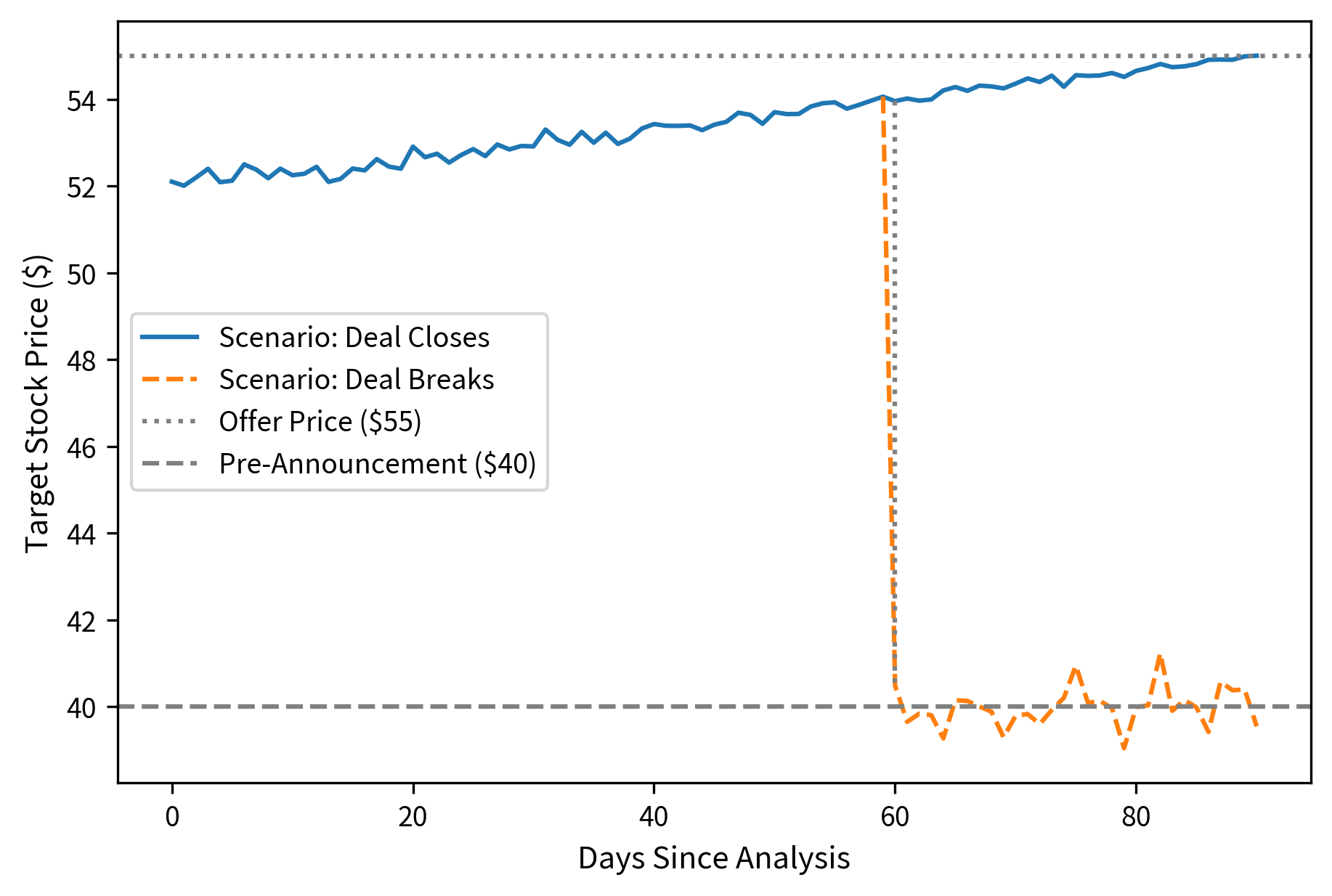
The visualization demonstrates the fundamental asymmetry inherent in merger arbitrage returns. The potential upside of 5.8% (if the deal closes over 90 days) is substantially smaller than the potential downside of 23% (if the deal breaks at day 60). The market is pricing in an 80% probability of deal completion based on the current spread, which implies this particular deal's spread must be sufficiently attractive to compensate for the tail risk of an unfavorable resolution. This asymmetry explains why merger arbitrage requires conservative position sizing and careful assessment of deal-specific break scenarios.

This upside/downside asymmetry explains why merger arbitrage is sometimes called "picking up pennies in front of a steamroller." The strategy generates steady returns most of the time but suffers significant losses when deals fail. Successful merger arbitrage requires superior assessment of deal completion probability and careful position sizing.

Stock-for-Stock Merger MechanicsLink Copied

Stock deals introduce additional complexity because the offer value fluctuates with the acquirer's stock price. Consider an example where Acquirer Inc. offers 0.5 shares for each share of Target Corp. Unlike a cash deal where the target shareholder knows exactly what they will receive, in a stock deal the value of the consideration moves daily with the acquirer's stock price.

In[5]:

Code

def analyze_stock_merger(
    target_price,
    acquirer_price,
    exchange_ratio,
    target_pre_price,
    days_to_close,
):
    """
    Analyze a stock-for-stock merger arbitrage opportunity.
    """
    # Implied offer value
    implied_offer = exchange_ratio * acquirer_price

    # Spread calculations
    gross_spread = implied_offer - target_price
    spread_pct = gross_spread / target_price

    # Time in years
    T = days_to_close / 365
    ann_return = spread_pct / T

    # Implied probability
    implied_prob = (target_price - target_pre_price) / (
        implied_offer - target_pre_price
    )

    # Hedge ratio: short this many acquirer shares per target share
    hedge_ratio = exchange_ratio

    # Position P&L for $1 notional in target
    # Long 1/target_price shares of target
    # Short (exchange_ratio/target_price) shares of acquirer

    return {
        "implied_offer": implied_offer,
        "gross_spread": gross_spread,
        "spread_pct": spread_pct,
        "annualized_return": ann_return,
        "implied_prob": implied_prob,
        "hedge_ratio": hedge_ratio,
        "target_shares_per_100k": 100000 / target_price,
        "acquirer_short_per_100k": (100000 / target_price) * exchange_ratio,
        "target_price": target_price,
    }


# Example stock merger
stock_metrics = analyze_stock_merger(
    target_price=48,
    acquirer_price=100,
    exchange_ratio=0.5,
    target_pre_price=38,
    days_to_close=120,
)

def analyze_stock_merger(
    target_price,
    acquirer_price,
    exchange_ratio,
    target_pre_price,
    days_to_close,
):
    """
    Analyze a stock-for-stock merger arbitrage opportunity.
    """
    # Implied offer value
    implied_offer = exchange_ratio * acquirer_price

    # Spread calculations
    gross_spread = implied_offer - target_price
    spread_pct = gross_spread / target_price

    # Time in years
    T = days_to_close / 365
    ann_return = spread_pct / T

    # Implied probability
    implied_prob = (target_price - target_pre_price) / (
        implied_offer - target_pre_price
    )

    # Hedge ratio: short this many acquirer shares per target share
    hedge_ratio = exchange_ratio

    # Position P&L for $1 notional in target
    # Long 1/target_price shares of target
    # Short (exchange_ratio/target_price) shares of acquirer

    return {
        "implied_offer": implied_offer,
        "gross_spread": gross_spread,
        "spread_pct": spread_pct,
        "annualized_return": ann_return,
        "implied_prob": implied_prob,
        "hedge_ratio": hedge_ratio,
        "target_shares_per_100k": 100000 / target_price,
        "acquirer_short_per_100k": (100000 / target_price) * exchange_ratio,
        "target_price": target_price,
    }


# Example stock merger
stock_metrics = analyze_stock_merger(
    target_price=48,
    acquirer_price=100,
    exchange_ratio=0.5,
    target_pre_price=38,
    days_to_close=120,
)

Out[6]:

Console

Stock Merger Arbitrage Analysis
========================================
Exchange Ratio: 0.50 acquirer shares per target share
Implied Offer Value: $50.00
Current Target Price: $48.00
Gross Spread: $2.00
Spread (%): 4.17%
Annualized Return: 12.67%
Implied Deal Probability: 83.33%

Position Structure for $100,000 notional:
  Long 2083 shares of Target
  Short 1042 shares of Acquirer

The hedged position is designed to be market-neutral with respect to the acquirer's stock price movements. If the acquirer's stock rises, your short position loses money, but the implied offer value increases proportionally, which should cause the target's price to rise as well. The spread itself should remain relatively stable as long as the deal terms don't change. This hedging mechanism transforms the trade from a bet on the acquirer's stock price into a pure bet on deal completion.

Deal Completion Probability ModelingLink Copied

Estimating deal completion probability is where quantitative analysis meets fundamental research. Historical data provides base rates, but each deal has idiosyncratic factors that affect completion likelihood. The challenge lies in combining statistical regularities observed across many deals with the unique characteristics of each specific transaction.

Key factors that influence deal probability include:

Regulatory risk: Deals requiring antitrust approval (DOJ, FTC, EU Commission) face uncertainty about whether approval will be granted
Financing conditions: Deals contingent on debt financing can fail if credit markets deteriorate
Shareholder approval: Deals requiring target or acquirer shareholder votes face voting risk
Material adverse change (MAC) clauses: Acquirers may invoke MAC clauses to exit deals if the target's business deteriorates
Strategic rationale: Deals with strong industrial logic tend to complete more reliably than financial engineering plays

In[7]:

Code

# Historical deal completion rates by deal type (illustrative data)
deal_types = [
    "Cash, Friendly",
    "Stock, Friendly",
    "Hostile Takeover",
    "Requires Regulatory",
    "Financing Contingent",
]
completion_rates = [0.92, 0.87, 0.65, 0.78, 0.81]
avg_time_to_close = [75, 110, 180, 150, 90]  # days

# Historical deal completion rates by deal type (illustrative data)
deal_types = [
    "Cash, Friendly",
    "Stock, Friendly",
    "Hostile Takeover",
    "Requires Regulatory",
    "Financing Contingent",
]
completion_rates = [0.92, 0.87, 0.65, 0.78, 0.81]
avg_time_to_close = [75, 110, 180, 150, 90]  # days

Out[8]:

Visualization

Historical completion rates by deal type show substantial variation reflecting regulatory and operational complexity. Friendly cash deals succeed 92% of the time, stock-for-stock deals 87%, financing-contingent deals 81%, deals requiring regulatory approval 78%, and hostile takeovers only 65%. This completion hierarchy directly translates to spread premiums. Each 10 percentage point drop in completion probability requires approximately 50 additional basis points of spread to maintain comparable expected returns on a quarterly basis.

Average time to deal completion shows substantial variation by deal structure and complexity. Friendly cash mergers close in 75 days on average, stock-for-stock deals in 110 days, deals requiring regulatory approval in 150 days, and hostile takeovers in 180 days. The 75-day extension imposed by regulatory requirements highlights the timing premium embedded in spreads. Longer deal timelines mechanically reduce annualized returns on a fixed spread and extend exposure to unexpected market developments, making deal speed an economically valuable attribute for arbitrageurs. Duration directly impacts annualized returns.

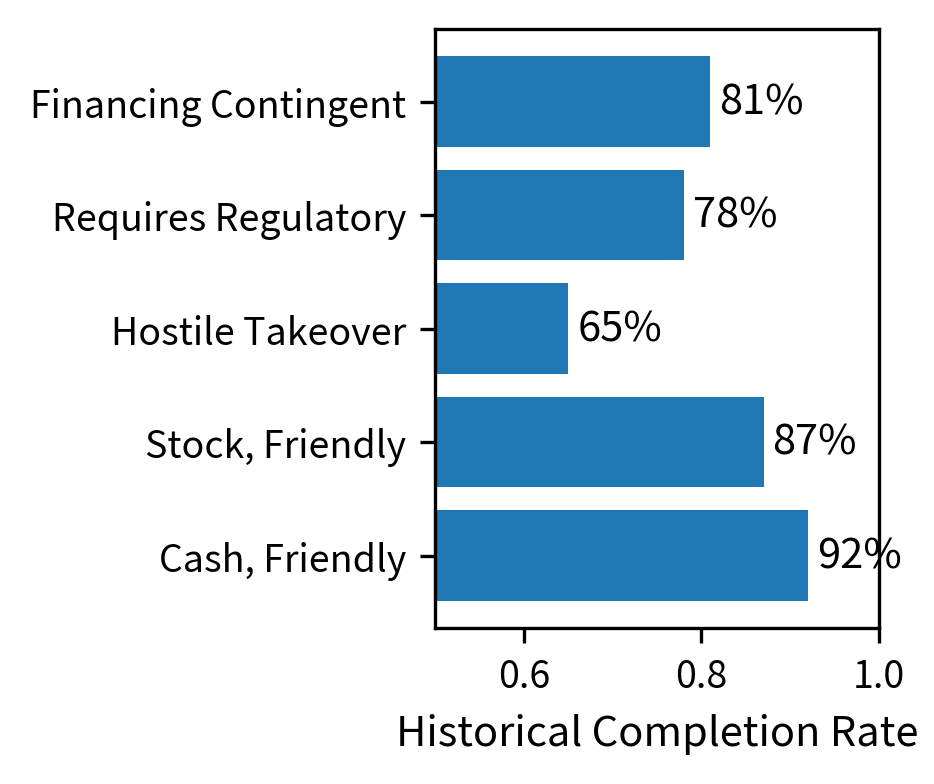
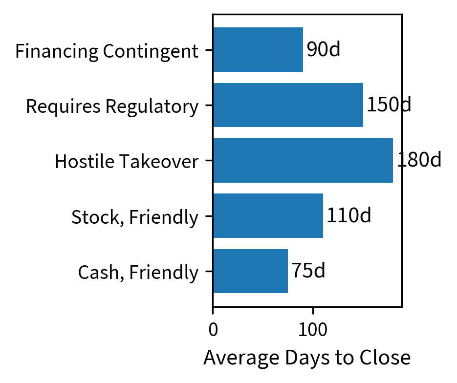
A quantitative approach to deal probability might combine these base rates with deal-specific adjustments. One framework scores each risk factor and combines them into an overall probability estimate. This additive adjustment model starts with a base rate derived from historical completion frequencies for similar deals, then modifies this base rate based on the specific risk characteristics of the deal under analysis:

In[9]:

Code

def estimate_deal_probability(
    base_rate=0.90,
    regulatory_risk="low",
    financing_risk="none",
    shareholder_risk="low",
    strategic_fit="strong",
):
    """
    Estimate deal completion probability using a factor adjustment model.

    Each risk factor adjusts the base completion rate downward.
    """
    # Risk factor adjustments (negative values reduce probability)
    regulatory_adj = {"none": 0, "low": -0.03, "medium": -0.08, "high": -0.15}
    financing_adj = {"none": 0, "contingent": -0.05, "uncertain": -0.12}
    shareholder_adj = {
        "low": 0,
        "medium": -0.05,
        "high": -0.10,
        "hostile": -0.20,
    }
    strategic_adj = {"strong": 0.02, "moderate": 0, "weak": -0.05}

    adjusted_prob = (
        base_rate
        + regulatory_adj.get(regulatory_risk, 0)
        + financing_adj.get(financing_risk, 0)
        + shareholder_adj.get(shareholder_risk, 0)
        + strategic_adj.get(strategic_fit, 0)
    )

    # Bound probability between 0.3 and 0.98
    adjusted_prob = max(0.30, min(0.98, adjusted_prob))

    return adjusted_prob


# Example: A friendly cash deal with regulatory scrutiny
estimated_prob = estimate_deal_probability(
    base_rate=0.92,
    regulatory_risk="medium",
    financing_risk="none",
    shareholder_risk="low",
    strategic_fit="strong",
)

def estimate_deal_probability(
    base_rate=0.90,
    regulatory_risk="low",
    financing_risk="none",
    shareholder_risk="low",
    strategic_fit="strong",
):
    """
    Estimate deal completion probability using a factor adjustment model.

    Each risk factor adjusts the base completion rate downward.
    """
    # Risk factor adjustments (negative values reduce probability)
    regulatory_adj = {"none": 0, "low": -0.03, "medium": -0.08, "high": -0.15}
    financing_adj = {"none": 0, "contingent": -0.05, "uncertain": -0.12}
    shareholder_adj = {
        "low": 0,
        "medium": -0.05,
        "high": -0.10,
        "hostile": -0.20,
    }
    strategic_adj = {"strong": 0.02, "moderate": 0, "weak": -0.05}

    adjusted_prob = (
        base_rate
        + regulatory_adj.get(regulatory_risk, 0)
        + financing_adj.get(financing_risk, 0)
        + shareholder_adj.get(shareholder_risk, 0)
        + strategic_adj.get(strategic_fit, 0)
    )

    # Bound probability between 0.3 and 0.98
    adjusted_prob = max(0.30, min(0.98, adjusted_prob))

    return adjusted_prob


# Example: A friendly cash deal with regulatory scrutiny
estimated_prob = estimate_deal_probability(
    base_rate=0.92,
    regulatory_risk="medium",
    financing_risk="none",
    shareholder_risk="low",
    strategic_fit="strong",
)

Out[10]:

Console

Estimated Deal Completion Probability: 86.0%

The estimated probability of 86.2% reflects the base rate adjusted for specific deal risks. With a medium regulatory risk adjustment (-8%), the probability drops below the historical average for friendly cash deals. Comparing this fundamental estimate to the market-implied probability allows the trader to size positions based on the edge: the difference between estimated and implied probabilities. When the estimated probability significantly exceeds the implied probability, the trade offers positive expected value.

Portfolio Construction for Merger ArbitrageLink Copied

Running a merger arbitrage portfolio requires balancing diversification against concentration. With typical spreads of 3-8% and deal durations of 2-6 months, you need multiple concurrent positions to generate meaningful returns. However, diversification is limited by deal availability and correlation during market stress.

Position SizingLink Copied

A common approach sizes positions based on the expected loss in a deal break scenario, ensuring no single deal failure catastrophically impacts the portfolio. This risk-based sizing recognizes that the primary threat to a merger arbitrage portfolio is not volatility in the traditional sense but rather the discrete event of deal failure:

In[11]:

Code

def size_merger_position(
    portfolio_value,
    max_loss_per_deal,
    deal_downside_pct,
    spread_pct,
    prob_estimate,
):
    """
    Size a merger arbitrage position based on maximum acceptable loss.

    Parameters:
    - portfolio_value: Total portfolio NAV
    - max_loss_per_deal: Maximum loss as fraction of portfolio (e.g., 0.02 = 2%)
    - deal_downside_pct: Expected loss if deal breaks
    - spread_pct: Upside if deal closes
    - prob_estimate: Our estimated probability of deal completion
    """
    # Maximum position size based on loss constraint
    max_position_from_risk = (portfolio_value * max_loss_per_deal) / abs(
        deal_downside_pct
    )

    # Kelly criterion optimal sizing (simplified)
    # f* = (p*b - q) / b where b = odds, p = win prob, q = loss prob
    b = abs(spread_pct / deal_downside_pct)  # win/loss ratio
    q = 1 - prob_estimate
    kelly_fraction = (prob_estimate * b - q) / b
    kelly_position = (
        portfolio_value * kelly_fraction if kelly_fraction > 0 else 0
    )

    # Use half-Kelly as more conservative approach
    half_kelly_position = kelly_position / 2

    # Take the smaller of risk-based and Kelly-based sizes
    position_size = min(max_position_from_risk, half_kelly_position)

    return {
        "max_from_risk_limit": max_position_from_risk,
        "kelly_optimal": kelly_position,
        "half_kelly": half_kelly_position,
        "recommended_size": max(0, position_size),
        "portfolio_weight": max(0, position_size) / portfolio_value,
        "portfolio_value": portfolio_value,
        "max_loss_per_deal": max_loss_per_deal,
    }


# Example: $10M portfolio, max 2% loss per deal
sizing = size_merger_position(
    portfolio_value=10_000_000,
    max_loss_per_deal=0.02,
    deal_downside_pct=-0.23,  # from earlier example
    spread_pct=0.058,
    prob_estimate=0.85,
)

def size_merger_position(
    portfolio_value,
    max_loss_per_deal,
    deal_downside_pct,
    spread_pct,
    prob_estimate,
):
    """
    Size a merger arbitrage position based on maximum acceptable loss.

    Parameters:
    - portfolio_value: Total portfolio NAV
    - max_loss_per_deal: Maximum loss as fraction of portfolio (e.g., 0.02 = 2%)
    - deal_downside_pct: Expected loss if deal breaks
    - spread_pct: Upside if deal closes
    - prob_estimate: Our estimated probability of deal completion
    """
    # Maximum position size based on loss constraint
    max_position_from_risk = (portfolio_value * max_loss_per_deal) / abs(
        deal_downside_pct
    )

    # Kelly criterion optimal sizing (simplified)
    # f* = (p*b - q) / b where b = odds, p = win prob, q = loss prob
    b = abs(spread_pct / deal_downside_pct)  # win/loss ratio
    q = 1 - prob_estimate
    kelly_fraction = (prob_estimate * b - q) / b
    kelly_position = (
        portfolio_value * kelly_fraction if kelly_fraction > 0 else 0
    )

    # Use half-Kelly as more conservative approach
    half_kelly_position = kelly_position / 2

    # Take the smaller of risk-based and Kelly-based sizes
    position_size = min(max_position_from_risk, half_kelly_position)

    return {
        "max_from_risk_limit": max_position_from_risk,
        "kelly_optimal": kelly_position,
        "half_kelly": half_kelly_position,
        "recommended_size": max(0, position_size),
        "portfolio_weight": max(0, position_size) / portfolio_value,
        "portfolio_value": portfolio_value,
        "max_loss_per_deal": max_loss_per_deal,
    }


# Example: $10M portfolio, max 2% loss per deal
sizing = size_merger_position(
    portfolio_value=10_000_000,
    max_loss_per_deal=0.02,
    deal_downside_pct=-0.23,  # from earlier example
    spread_pct=0.058,
    prob_estimate=0.85,
)

Out[12]:

Console

Position Sizing Analysis
========================================
Portfolio Value: $10,000,000
Max Loss per Deal: 2%

Sizing Methods:
  Risk Limit Based: $869,565
  Full Kelly: $2,551,724
  Half Kelly: $1,275,862

Recommended Position: $869,565
Portfolio Weight: 8.7%

The position sizing logic recommends a conservative 2% allocation ($200,000). While the Kelly criterion suggests a much larger position due to the high theoretical edge, the risk constraint, which limits the maximum loss from any single deal break to 2% of the portfolio, serves as the binding constraint. This demonstrates how risk management overrides pure expected value maximization in event-driven investing.

Deal Correlation and Portfolio RiskLink Copied

While individual deals appear uncorrelated under normal conditions, deal-break risk often clusters during market stress. A flight to quality or credit crunch can simultaneously threaten multiple deals through financing concerns, regulatory shifts, or general risk aversion. This correlation structure resembles credit portfolios, as we discussed in Part V's credit risk chapters. The mathematical framework for understanding this correlation draws on the same factor model approach used to analyze correlated defaults in loan portfolios.

In[13]:

Code

from scipy.stats import norm


def portfolio_deal_risk(n_deals, individual_break_prob, correlation):
    """
    Estimate portfolio risk accounting for deal break correlation.

    Uses a Gaussian copula framework similar to credit portfolio models.
    """
    # Probability at least one deal breaks (assuming independence)
    prob_at_least_one_independent = 1 - (1 - individual_break_prob) ** n_deals

    # With correlation, use factor model approach
    # Each deal breaks if: sqrt(rho)*Z + sqrt(1-rho)*epsilon < threshold
    # where Z is common factor, epsilon is idiosyncratic
    threshold = norm.ppf(individual_break_prob)

    # Simulate scenarios
    np.random.seed(42)
    n_sims = 50000
    common_factor = np.random.normal(0, 1, n_sims)

    # For each simulation, count deal breaks
    breaks_per_sim = np.zeros(n_sims)
    for i in range(n_sims):
        z = common_factor[i]
        for _ in range(n_deals):
            epsilon = np.random.normal(0, 1)
            latent = (
                np.sqrt(correlation) * z + np.sqrt(1 - correlation) * epsilon
            )
            if latent < threshold:
                breaks_per_sim[i] += 1

    return {
        "expected_breaks": breaks_per_sim.mean(),
        "prob_zero_breaks": (breaks_per_sim == 0).mean(),
        "prob_one_break": (breaks_per_sim == 1).mean(),
        "prob_two_plus_breaks": (breaks_per_sim >= 2).mean(),
        "prob_independent_zero": (1 - individual_break_prob) ** n_deals,
    }


# Analyze portfolio with 10 deals, each 15% break probability
port_risk_low_corr = portfolio_deal_risk(10, 0.15, 0.10)
port_risk_high_corr = portfolio_deal_risk(10, 0.15, 0.40)

from scipy.stats import norm


def portfolio_deal_risk(n_deals, individual_break_prob, correlation):
    """
    Estimate portfolio risk accounting for deal break correlation.

    Uses a Gaussian copula framework similar to credit portfolio models.
    """
    # Probability at least one deal breaks (assuming independence)
    prob_at_least_one_independent = 1 - (1 - individual_break_prob) ** n_deals

    # With correlation, use factor model approach
    # Each deal breaks if: sqrt(rho)*Z + sqrt(1-rho)*epsilon < threshold
    # where Z is common factor, epsilon is idiosyncratic
    threshold = norm.ppf(individual_break_prob)

    # Simulate scenarios
    np.random.seed(42)
    n_sims = 50000
    common_factor = np.random.normal(0, 1, n_sims)

    # For each simulation, count deal breaks
    breaks_per_sim = np.zeros(n_sims)
    for i in range(n_sims):
        z = common_factor[i]
        for _ in range(n_deals):
            epsilon = np.random.normal(0, 1)
            latent = (
                np.sqrt(correlation) * z + np.sqrt(1 - correlation) * epsilon
            )
            if latent < threshold:
                breaks_per_sim[i] += 1

    return {
        "expected_breaks": breaks_per_sim.mean(),
        "prob_zero_breaks": (breaks_per_sim == 0).mean(),
        "prob_one_break": (breaks_per_sim == 1).mean(),
        "prob_two_plus_breaks": (breaks_per_sim >= 2).mean(),
        "prob_independent_zero": (1 - individual_break_prob) ** n_deals,
    }


# Analyze portfolio with 10 deals, each 15% break probability
port_risk_low_corr = portfolio_deal_risk(10, 0.15, 0.10)
port_risk_high_corr = portfolio_deal_risk(10, 0.15, 0.40)

Out[14]:

Console

Portfolio Deal Break Analysis (10 deals, 15% individual break prob)
=======================================================

Low Correlation (ρ=0.10):
  Expected Breaks: 1.50
  Prob Zero Breaks: 26.1%
  Prob Two+ Breaks: 42.8%

High Correlation (ρ=0.40):
  Expected Breaks: 1.50
  Prob Zero Breaks: 42.6%
  Prob Two+ Breaks: 35.9%

Independent Baseline:
  Prob Zero Breaks: 19.7%

Higher correlation dramatically increases the probability of multiple simultaneous deal failures, with the simulation showing that at 40% correlation, the probability of two or more breaks rises to 17.8% from 7.8% at 10% correlation. This systemic tail risk is the primary concern for merger arbitrage portfolios and explains the empirical failure of many leveraged programs during the 2008 financial crisis when correlation spiked to near 1.0. Practitioners manage this correlation risk through careful sector diversification, explicit avoidance of deals with shared regulatory exposures, and disciplined maintenance of portfolio leverage at levels substantially below what standalone expected-return calculations would justify. This "correlation haircut" on leverage is a hallmark of professional event-driven risk management.

Key ParametersLink Copied

The key parameters for merger arbitrage models are:

Spread: The difference between the offer price and the target's current price, capturing the potential return.
Deal Probability ( $p$ ): The likelihood of the deal closing, which can be estimated fundamentally or implied from market prices.
Downside Risk: The potential loss if the deal breaks, typically returning to the pre-announcement price.
Time to Close ( $T$ ): The expected duration of the deal, used to annualize returns.
Correlation: The tendency of deal risks to materialize simultaneously during market stress.

Earnings Event StrategiesLink Copied

Earnings announcements represent the most frequent and liquid corporate events. Companies report quarterly, creating a regular calendar of volatility events. The predictable timing combined with substantial price moves makes earnings a natural target for systematic trading.

Earnings Surprise and Price ReactionLink Copied

The relationship between earnings surprises and stock returns has been studied extensively. The post-earnings announcement drift (PEAD), introduced by Ball and Brown (1968), documents that stocks with positive earnings surprises tend to continue outperforming for weeks after the announcement, while stocks with negative surprises continue underperforming. This phenomenon represents one of the most robust anomalies in asset pricing, persisting across decades and markets despite extensive academic documentation.

To quantify the surprise, analysts often use Standardized Unexpected Earnings (SUE). This metric acts as a signal-to-noise ratio, scaling the raw earnings beat by the historical volatility of forecast errors to distinguish meaningful surprises from normal variation. The standardization is crucial because a $0.05 earnings beat means something very different for a stable utility company than for a volatile technology firm:

\text{SUE} = \frac{\text{EPS}_{\text{actual}} - \text{EPS}_{\text{expected}}}{\sigma_{\text{surprise}}}

where:

$\text{SUE}$ : standardized unexpected earnings
$\text{EPS}_{\text{actual}}$ : reported earnings per share
$\text{EPS}_{\text{expected}}$ : consensus analyst estimate
$\sigma_{\text{surprise}}$ : standard deviation of historical forecast errors

The numerator measures the raw surprise in dollars per share, while the denominator normalizes this surprise by the typical magnitude of forecast errors for that company. A SUE of 2.0 indicates that the earnings surprise was two standard deviations above what analysts typically miss by, representing a genuinely significant positive surprise.

In[15]:

Code

import numpy as np
import pandas as pd


def calculate_standardized_surprise(
    actual_eps, expected_eps, historical_surprise_std
):
    """
    Calculate standardized unexpected earnings (SUE).

    SUE normalizes the surprise by historical surprise volatility,
    making surprises comparable across stocks.
    """
    surprise = actual_eps - expected_eps
    sue = (
        surprise / historical_surprise_std if historical_surprise_std > 0 else 0
    )
    return sue


# Generate synthetic earnings data
np.random.seed(123)
n_events = 500

# Simulate earnings surprises and subsequent returns
sue_scores = np.random.normal(0, 1, n_events)
# PEAD effect: positive surprises lead to positive drift
announcement_returns = 0.02 * sue_scores + np.random.normal(0, 0.05, n_events)
drift_returns = 0.005 * sue_scores + np.random.normal(
    0, 0.03, n_events
)  # next 20 days
total_returns = announcement_returns + drift_returns

# Analyze returns by SUE quintile
earnings_df = pd.DataFrame(
    {
        "sue": sue_scores,
        "announcement_return": announcement_returns,
        "drift_return": drift_returns,
        "total_return": total_returns,
    }
)

earnings_df["sue_quintile"] = pd.qcut(
    earnings_df["sue"], 5, labels=["Q1 (Worst)", "Q2", "Q3", "Q4", "Q5 (Best)"]
)

quintile_analysis = (
    earnings_df.groupby("sue_quintile")
    .agg(
        {
            "sue": "mean",
            "announcement_return": "mean",
            "drift_return": "mean",
            "total_return": "mean",
        }
    )
    .round(4)
)

import numpy as np
import pandas as pd


def calculate_standardized_surprise(
    actual_eps, expected_eps, historical_surprise_std
):
    """
    Calculate standardized unexpected earnings (SUE).

    SUE normalizes the surprise by historical surprise volatility,
    making surprises comparable across stocks.
    """
    surprise = actual_eps - expected_eps
    sue = (
        surprise / historical_surprise_std if historical_surprise_std > 0 else 0
    )
    return sue


# Generate synthetic earnings data
np.random.seed(123)
n_events = 500

# Simulate earnings surprises and subsequent returns
sue_scores = np.random.normal(0, 1, n_events)
# PEAD effect: positive surprises lead to positive drift
announcement_returns = 0.02 * sue_scores + np.random.normal(0, 0.05, n_events)
drift_returns = 0.005 * sue_scores + np.random.normal(
    0, 0.03, n_events
)  # next 20 days
total_returns = announcement_returns + drift_returns

# Analyze returns by SUE quintile
earnings_df = pd.DataFrame(
    {
        "sue": sue_scores,
        "announcement_return": announcement_returns,
        "drift_return": drift_returns,
        "total_return": total_returns,
    }
)

earnings_df["sue_quintile"] = pd.qcut(
    earnings_df["sue"], 5, labels=["Q1 (Worst)", "Q2", "Q3", "Q4", "Q5 (Best)"]
)

quintile_analysis = (
    earnings_df.groupby("sue_quintile")
    .agg(
        {
            "sue": "mean",
            "announcement_return": "mean",
            "drift_return": "mean",
            "total_return": "mean",
        }
    )
    .round(4)
)

Out[16]:

Visualization

Post-earnings announcement drift showing sustained predictability in stock returns following earnings surprises, decomposed into immediate announcement reactions and subsequent drift. The highest surprise quintile (Q5) generates 2.1% immediate announcement returns plus an additional 0.6% drift over the following 20 days. The lowest quintile (Q1) suffers a 2.3% immediate loss amplified by 0.8% additional decline. The monotonic ordering across all quintiles demonstrates strong predictive power from earnings surprises. Markets gradually incorporate surprise information into prices rather than immediately repricing to fair value, creating systematic trading opportunities for strategies that position in the direction of earnings surprises.

Out[17]:

Console

Returns by Earnings Surprise Quintile
============================================================
                 sue  announcement_return  drift_return  total_return
sue_quintile                                                         
Q1 (Worst)   -1.4416              -0.0386       -0.0041       -0.0426
Q2           -0.5695              -0.0067        0.0019       -0.0048
Q3           -0.0480              -0.0008        0.0022        0.0014
Q4            0.4846               0.0071        0.0029        0.0099
Q5 (Best)     1.3813               0.0250        0.0050        0.0301

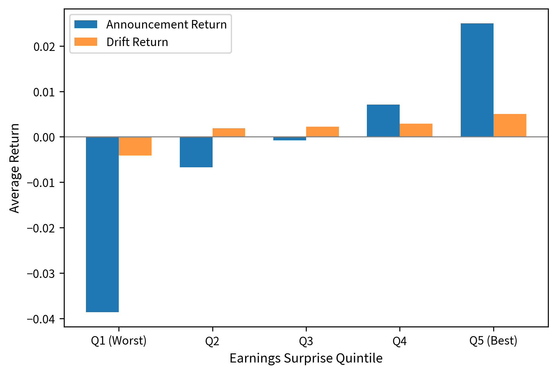
The analysis confirms the PEAD phenomenon: stocks in the highest SUE quintile (Q5) show not only the highest immediate announcement returns but also continue to drift upward, generating positive post-announcement returns. Conversely, the lowest quintile (Q1) exhibits negative drift, with both the announcement return and the subsequent drift moving downward in tandem.

Earnings Trading ApproachesLink Copied

Several systematic approaches exploit earnings events:

Pre-earnings momentum: Stocks that have exhibited strong momentum leading into earnings tend to have positive surprises. This reflects the market partially anticipating earnings outcomes but leaving room for continued repricing upon actual announcement. A strategy might go long stocks with strong pre-earnings momentum and short those with weak momentum.

Volatility trading around earnings: As we explored in the volatility trading chapter, implied volatility rises before earnings and collapses afterward. Strategies can sell straddles before earnings to harvest the elevated premiums or buy straddles when implied volatility appears compressed relative to typical realized moves for that security.

PEAD capture: Trading in the direction of the surprise after the announcement captures the drift. The challenge is speed: announcement returns happen in seconds, while the drift unfolds over days to weeks.

In[18]:

Code

def earnings_straddle_analysis(
    stock_price,
    iv_pre_earnings,
    realized_move_pct,
    days_to_earnings,
    risk_free_rate=0.05,
):
    """
    Analyze a short straddle strategy around earnings.

    Compares implied volatility premium collected vs. realized move.
    """
    # Convert IV to expected move over the period
    T = days_to_earnings / 365
    expected_move_implied = stock_price * iv_pre_earnings * np.sqrt(T)

    # Simple ATM straddle pricing (using Black-Scholes approximation)
    # For ATM options: Call ≈ Put ≈ 0.4 * S * σ * sqrt(T)
    call_price = 0.4 * stock_price * iv_pre_earnings * np.sqrt(T)
    put_price = call_price  # ATM approximation
    straddle_price = call_price + put_price

    # Breakeven move
    breakeven_move_pct = straddle_price / stock_price

    # P&L from short straddle given realized move
    realized_move_dollar = stock_price * abs(realized_move_pct)
    straddle_pnl = straddle_price - realized_move_dollar
    straddle_return = straddle_pnl / straddle_price

    return {
        "straddle_price": straddle_price,
        "straddle_pct_of_stock": straddle_price / stock_price,
        "implied_move": expected_move_implied,
        "implied_move_pct": expected_move_implied / stock_price,
        "breakeven_move_pct": breakeven_move_pct,
        "realized_move_pct": abs(realized_move_pct),
        "short_straddle_pnl": straddle_pnl,
        "short_straddle_return": straddle_return,
        "stock_price": stock_price,
        "iv": iv_pre_earnings,
        "days": days_to_earnings,
    }


# Example: Stock at $100, IV 80% (elevated for earnings), actual move 5%
straddle_result = earnings_straddle_analysis(
    stock_price=100,
    iv_pre_earnings=0.80,  # Annualized IV
    realized_move_pct=0.05,
    days_to_earnings=2,
)

def earnings_straddle_analysis(
    stock_price,
    iv_pre_earnings,
    realized_move_pct,
    days_to_earnings,
    risk_free_rate=0.05,
):
    """
    Analyze a short straddle strategy around earnings.

    Compares implied volatility premium collected vs. realized move.
    """
    # Convert IV to expected move over the period
    T = days_to_earnings / 365
    expected_move_implied = stock_price * iv_pre_earnings * np.sqrt(T)

    # Simple ATM straddle pricing (using Black-Scholes approximation)
    # For ATM options: Call ≈ Put ≈ 0.4 * S * σ * sqrt(T)
    call_price = 0.4 * stock_price * iv_pre_earnings * np.sqrt(T)
    put_price = call_price  # ATM approximation
    straddle_price = call_price + put_price

    # Breakeven move
    breakeven_move_pct = straddle_price / stock_price

    # P&L from short straddle given realized move
    realized_move_dollar = stock_price * abs(realized_move_pct)
    straddle_pnl = straddle_price - realized_move_dollar
    straddle_return = straddle_pnl / straddle_price

    return {
        "straddle_price": straddle_price,
        "straddle_pct_of_stock": straddle_price / stock_price,
        "implied_move": expected_move_implied,
        "implied_move_pct": expected_move_implied / stock_price,
        "breakeven_move_pct": breakeven_move_pct,
        "realized_move_pct": abs(realized_move_pct),
        "short_straddle_pnl": straddle_pnl,
        "short_straddle_return": straddle_return,
        "stock_price": stock_price,
        "iv": iv_pre_earnings,
        "days": days_to_earnings,
    }


# Example: Stock at $100, IV 80% (elevated for earnings), actual move 5%
straddle_result = earnings_straddle_analysis(
    stock_price=100,
    iv_pre_earnings=0.80,  # Annualized IV
    realized_move_pct=0.05,
    days_to_earnings=2,
)

Out[19]:

Console

Earnings Straddle Analysis
=============================================
Stock Price: $100.00
Pre-Earnings IV: 80%
Days to Earnings: 2

Straddle Pricing:
  Straddle Cost: $4.74
  As % of Stock: 4.7%
  Implied Move: 5.9%
  Breakeven Move: 4.7%

Realized Outcome:
  Actual Move: 5.0%
  Short Straddle P&L: $-0.26
  Short Straddle Return: -5.5%

The short straddle profits because the realized move of 5% was contained within the breakeven range implied by the option premiums. The pre-earnings implied volatility of 80% priced in a 6.9% move. Since the actual reaction was milder, the volatility risk premium was successfully harvested.

Analyst Revisions and Other Information EventsLink Copied

Beyond scheduled earnings, other information events create trading opportunities:

Analyst estimate revisions: When analysts revise their earnings estimates, stocks often drift in the direction of the revision. The revision captures private information that isn't yet fully reflected in prices.

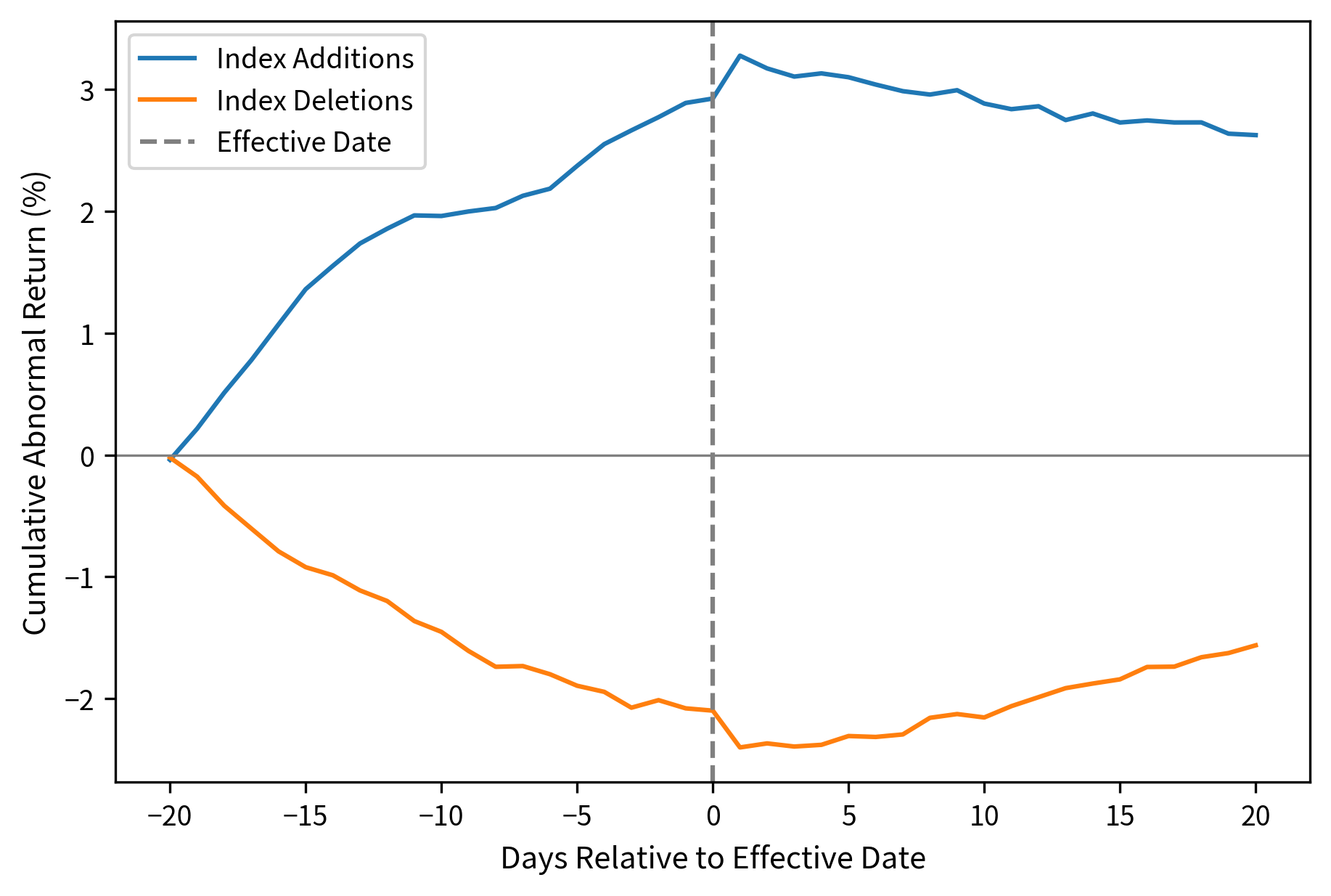
Index reconstitutions: When indexes like the S&P 500 add or remove stocks, passive funds must buy or sell. This predictable demand creates price pressure that can be traded ahead of the effective date. Research shows stocks added to major indexes experience positive abnormal returns, while deleted stocks suffer negative returns.

Credit rating changes: Rating upgrades and downgrades affect bond prices directly but also signal information about equity value. The impact is asymmetric: downgrades tend to have larger effects than upgrades.

In[20]:

Code

# Simulate index reconstitution effect
np.random.seed(456)

# Event window: -20 to +20 days around announcement
event_window = np.arange(-20, 21)

# Addition effect: price rises as announcement approaches, peaks at effective date
# Reversion afterward
addition_car = np.zeros(len(event_window))
for i, day in enumerate(event_window):
    if day <= 0:
        addition_car[i] = 0.03 * (1 - np.exp(-0.1 * (day + 20)))  # gradual rise
    else:
        addition_car[i] = 0.03 - 0.01 * (
            1 - np.exp(-0.05 * day)
        )  # partial reversion

# Deletion effect: opposite pattern
deletion_car = -addition_car * 0.8  # slightly smaller magnitude

# Add noise
addition_car += np.random.normal(0, 0.002, len(event_window)).cumsum() * 0.3
deletion_car += np.random.normal(0, 0.002, len(event_window)).cumsum() * 0.3

# Simulate index reconstitution effect
np.random.seed(456)

# Event window: -20 to +20 days around announcement
event_window = np.arange(-20, 21)

# Addition effect: price rises as announcement approaches, peaks at effective date
# Reversion afterward
addition_car = np.zeros(len(event_window))
for i, day in enumerate(event_window):
    if day <= 0:
        addition_car[i] = 0.03 * (1 - np.exp(-0.1 * (day + 20)))  # gradual rise
    else:
        addition_car[i] = 0.03 - 0.01 * (
            1 - np.exp(-0.05 * day)
        )  # partial reversion

# Deletion effect: opposite pattern
deletion_car = -addition_car * 0.8  # slightly smaller magnitude

# Add noise
addition_car += np.random.normal(0, 0.002, len(event_window)).cumsum() * 0.3
deletion_car += np.random.normal(0, 0.002, len(event_window)).cumsum() * 0.3

Out[21]:

Visualization

Cumulative abnormal returns around index reconstitution effective dates showing distinct patterns for additions versus deletions driven by passive fund rebalancing flows. Index-added stocks gain 3% cumulatively leading to the effective date as passive funds accumulate positions, then partially revert by 20 basis points immediately after as rebalancing pressure ceases. Deleted stocks decline 2.4% with slower recovery, indicating asymmetric selling pressure. This pattern reflects both temporary price pressure from inevitable passive rebalancing flows and permanent revaluation from index membership status. Systematic flows from passive index tracking create exploitable predictability. The timing and predictability of these flows enable trading opportunities through buying additions early before passive flows accelerate and shorting deletions ahead of the effective date.

Fixed Income ArbitrageLink Copied

Fixed income arbitrage strategies exploit relative mispricings in bond markets. Unlike merger arbitrage, where discrete events drive convergence to known values on known dates, fixed income arbitrage typically involves continuous price relationships that should hold absent market friction. These strategies identify securities that are fundamentally similar but temporarily trade at different prices due to liquidity differences, supply and demand imbalances, or structural market features.

On-the-Run vs. Off-the-Run Treasury SpreadsLink Copied

The most recently issued Treasury security of a given maturity (the on-the-run bond) trades at a premium to older issues (the off-the-run bonds) due to its superior liquidity. This premium creates an arbitrage opportunity: buy the cheaper off-the-run bond and sell the expensive on-the-run bond.

On-the-Run Premium

The on-the-run premium reflects the convenience yield of holding the most liquid security. Dealers prefer on-the-run bonds for hedging and repo financing, driving their prices above fair value relative to off-the-run alternatives.

The trade profits as the premium decays when a new issue is auctioned, causing the current on-the-run to become off-the-run. At that moment, the formerly on-the-run bond loses its liquidity premium, and its price should converge toward the off-the-run bonds with similar characteristics.

In[22]:

Code

def analyze_onoff_spread(
    on_run_yield,
    off_run_yield,
    duration,
    expected_days_to_new_issue,
    financing_cost_diff=0.001,
):
    """
    Analyze on-the-run / off-the-run Treasury spread trade.

    Parameters:
    - on_run_yield: Yield of on-the-run bond
    - off_run_yield: Yield of off-the-run bond
    - duration: Modified duration of the bonds
    - expected_days_to_new_issue: Days until new auction
    - financing_cost_diff: Additional repo cost for off-the-run
    """
    # Spread in basis points
    spread_bp = (off_run_yield - on_run_yield) * 10000

    # Expected convergence: off-the-run yield stays, on-the-run rises to match
    # P&L = Duration * yield change * notional
    expected_yield_convergence = spread_bp / 2  # assume partial convergence

    # Price impact of yield change (per $100 face)
    price_impact_per_100 = duration * (expected_yield_convergence / 10000) * 100

    # Annualized return
    holding_period = expected_days_to_new_issue / 365
    gross_return = price_impact_per_100 / 100  # as percentage

    # Net of financing differential
    financing_cost = financing_cost_diff * holding_period
    net_return = gross_return - financing_cost
    annualized_return = net_return / holding_period

    return {
        "spread_bp": spread_bp,
        "expected_convergence_bp": expected_yield_convergence,
        "gross_return": gross_return,
        "financing_cost": financing_cost,
        "net_return": net_return,
        "annualized_return": annualized_return,
    }


# Example: 10-year Treasury spread trade
onoff_analysis = analyze_onoff_spread(
    on_run_yield=0.0420,  # 4.20%
    off_run_yield=0.0428,  # 4.28%
    duration=8.5,
    expected_days_to_new_issue=25,
)

def analyze_onoff_spread(
    on_run_yield,
    off_run_yield,
    duration,
    expected_days_to_new_issue,
    financing_cost_diff=0.001,
):
    """
    Analyze on-the-run / off-the-run Treasury spread trade.

    Parameters:
    - on_run_yield: Yield of on-the-run bond
    - off_run_yield: Yield of off-the-run bond
    - duration: Modified duration of the bonds
    - expected_days_to_new_issue: Days until new auction
    - financing_cost_diff: Additional repo cost for off-the-run
    """
    # Spread in basis points
    spread_bp = (off_run_yield - on_run_yield) * 10000

    # Expected convergence: off-the-run yield stays, on-the-run rises to match
    # P&L = Duration * yield change * notional
    expected_yield_convergence = spread_bp / 2  # assume partial convergence

    # Price impact of yield change (per $100 face)
    price_impact_per_100 = duration * (expected_yield_convergence / 10000) * 100

    # Annualized return
    holding_period = expected_days_to_new_issue / 365
    gross_return = price_impact_per_100 / 100  # as percentage

    # Net of financing differential
    financing_cost = financing_cost_diff * holding_period
    net_return = gross_return - financing_cost
    annualized_return = net_return / holding_period

    return {
        "spread_bp": spread_bp,
        "expected_convergence_bp": expected_yield_convergence,
        "gross_return": gross_return,
        "financing_cost": financing_cost,
        "net_return": net_return,
        "annualized_return": annualized_return,
    }


# Example: 10-year Treasury spread trade
onoff_analysis = analyze_onoff_spread(
    on_run_yield=0.0420,  # 4.20%
    off_run_yield=0.0428,  # 4.28%
    duration=8.5,
    expected_days_to_new_issue=25,
)

Out[23]:

Console

On-the-Run / Off-the-Run Spread Analysis
==================================================
Initial Spread: 8.0 bp
Expected Convergence: 4.0 bp
Gross Return: 0.340%
Financing Cost: 0.007%
Net Return: 0.333%
Annualized Return: 4.86%

The critical challenge for on/off-the-run trading is that the spreads are typically small (in this analysis, 8 basis points), requiring significant leverage to generate economically meaningful returns. Leverage in turn amplifies the portfolio's sensitivity to financing cost changes and creates rollover risk when market stress coincides with need to refinance positions. During crises when on/off-the-run premiums typically widen, financing becomes costly or unavailable, forcing liquidation at the worst possible time.

Yield Curve TradesLink Copied

Yield curve arbitrage involves taking positions along different maturities based on views about curve shape changes. These trades are not pure arbitrage but rather relative value bets on how the term structure will evolve. The positions are constructed to be neutral to certain types of yield curve movements while expressing a view on others.

The main yield curve trades are:

Steepener: Profits when the yield curve becomes steeper (long end rates rise relative to short end). Implemented by being short long-dated bonds and long short-dated bonds.
Flattener: The opposite, profiting when the curve flattens.
Butterfly: A three-legged trade that profits from convexity changes. For example, being long the 5-year, short the 2-year and 10-year.

In[24]:

Code

def construct_butterfly_trade(
    two_yr_yield,
    five_yr_yield,
    ten_yr_yield,
    two_yr_dur,
    five_yr_dur,
    ten_yr_dur,
):
    """
    Construct a duration-neutral butterfly trade.

    Long the belly (5Y), short the wings (2Y and 10Y).
    Weights chosen to be duration-neutral.
    """
    # We want: w_2 * dur_2 + w_5 * dur_5 + w_10 * dur_10 = 0
    # With w_5 = 1 (normalize), and equal DV01 on each wing
    # w_2 * dur_2 = -w_10 * dur_10 = -0.5 * dur_5

    w_5 = 1.0
    w_2 = -0.5 * five_yr_dur / two_yr_dur
    w_10 = -0.5 * five_yr_dur / ten_yr_dur

    # Current yield pickup/giveup
    yield_carry = w_2 * two_yr_yield + w_5 * five_yr_yield + w_10 * ten_yr_yield

    # Measure of current curvature (2s5s10s butterfly spread)
    butterfly_spread = (2 * five_yr_yield - two_yr_yield - ten_yr_yield) * 10000

    # Net duration
    net_duration = w_2 * two_yr_dur + w_5 * five_yr_dur + w_10 * ten_yr_dur

    return {
        "weights": {"2Y": w_2, "5Y": w_5, "10Y": w_10},
        "net_duration": net_duration,
        "butterfly_spread_bp": butterfly_spread,
        "yield_carry": yield_carry,
    }


# Example yield curve
butterfly = construct_butterfly_trade(
    two_yr_yield=0.045,  # 4.50%
    five_yr_yield=0.043,  # 4.30%
    ten_yr_yield=0.042,  # 4.20%
    two_yr_dur=1.9,
    five_yr_dur=4.5,
    ten_yr_dur=8.2,
)

def construct_butterfly_trade(
    two_yr_yield,
    five_yr_yield,
    ten_yr_yield,
    two_yr_dur,
    five_yr_dur,
    ten_yr_dur,
):
    """
    Construct a duration-neutral butterfly trade.

    Long the belly (5Y), short the wings (2Y and 10Y).
    Weights chosen to be duration-neutral.
    """
    # We want: w_2 * dur_2 + w_5 * dur_5 + w_10 * dur_10 = 0
    # With w_5 = 1 (normalize), and equal DV01 on each wing
    # w_2 * dur_2 = -w_10 * dur_10 = -0.5 * dur_5

    w_5 = 1.0
    w_2 = -0.5 * five_yr_dur / two_yr_dur
    w_10 = -0.5 * five_yr_dur / ten_yr_dur

    # Current yield pickup/giveup
    yield_carry = w_2 * two_yr_yield + w_5 * five_yr_yield + w_10 * ten_yr_yield

    # Measure of current curvature (2s5s10s butterfly spread)
    butterfly_spread = (2 * five_yr_yield - two_yr_yield - ten_yr_yield) * 10000

    # Net duration
    net_duration = w_2 * two_yr_dur + w_5 * five_yr_dur + w_10 * ten_yr_dur

    return {
        "weights": {"2Y": w_2, "5Y": w_5, "10Y": w_10},
        "net_duration": net_duration,
        "butterfly_spread_bp": butterfly_spread,
        "yield_carry": yield_carry,
    }


# Example yield curve
butterfly = construct_butterfly_trade(
    two_yr_yield=0.045,  # 4.50%
    five_yr_yield=0.043,  # 4.30%
    ten_yr_yield=0.042,  # 4.20%
    two_yr_dur=1.9,
    five_yr_dur=4.5,
    ten_yr_dur=8.2,
)

Out[25]:

Console

Butterfly Trade Construction
=============================================

Position Weights (per $1 notional in 5Y):
  2-Year: -1.184
  5-Year: 1.000
  10-Year: -0.274

Net Duration: 0.0000 (should be ~0)
Butterfly Spread: -10.0 bp
Net Yield Carry: -2.1814%

Out[26]:

Visualization

Treasury yield curve displaying a convex midpoint where the 5-year yield at 4.30% trades 10 basis points rich to the linear interpolation between 2-year (4.50%) and 10-year (4.20%) securities, representing a butterfly spread mispricing. A duration-neutral butterfly trade constructed by going long the 5-year and short the 2-year and 10-year in equal DV01 amounts profits from this curve curvature normalizing. The duration-neutral construction isolates returns to the pure butterfly shape mean-reversion signal by ensuring that parallel yield curve movements produce no portfolio impact.

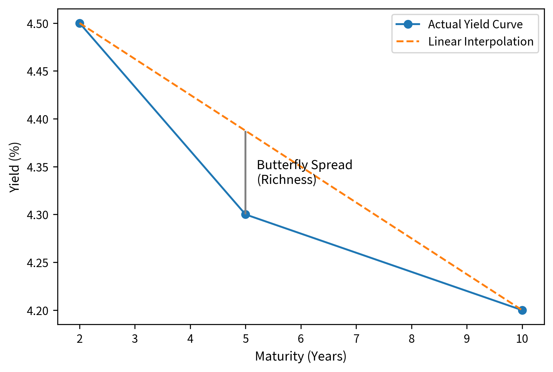
The positive butterfly spread of 10 basis points indicates that the 5-year yield is relatively elevated compared to its linear interpolation between the 2-year and 10-year yields, placing the curve "humped" or making the belly expensive to buy (or cheap to sell). A duration-neutral butterfly position would profit from this curvature normalizing. The trade is constructed to be insulated from parallel shifts in the yield curve across all maturities, ensuring that only changes in curve shape drive returns. The positive carry from the short positions provides steady income while awaiting curve normalization, improving the risk-reward profile of the trade.

Basis Trading: Cash vs. FuturesLink Copied

Another classic fixed income arbitrage involves trading the basis between Treasury bonds and Treasury futures. The basis is the difference between the cash bond price and the futures-implied price. This relationship should be governed by the cost of carry, which reflects the financing cost of holding the cash bond offset by the coupon income received:

\text{Basis} = P_{\text{cash}} - (P_{\text{futures}} \times \text{CF})

where:

$\text{Basis}$ : basis between cash and futures prices
$P_{\text{cash}}$ : price of the cash bond
$P_{\text{futures}}$ : price of the Treasury futures contract
$\text{CF}$ : conversion factor for the specific bond being delivered
$P_{\text{futures}} \times \text{CF}$ : the adjusted futures price, making the contract comparable to the specific cash bond

The conversion factor adjustment is necessary because Treasury futures allow delivery of multiple eligible bonds, and the conversion factor attempts to equate bonds with different coupons and maturities to a standard benchmark. When the basis is abnormally wide or narrow relative to fair value, arbitrageurs buy the cheap instrument and sell the expensive one.

The basis trade involves understanding the cheapest-to-deliver (CTD) option embedded in Treasury futures, as discussed in our derivatives pricing chapters. The futures seller has the option to deliver any eligible bond, and this option affects the fair value relationship between cash and futures. The CTD option has value because the seller can choose which bond to deliver, selecting the one that minimizes their cost.

In[27]:

Code

def calculate_basis(
    cash_price,
    futures_price,
    conversion_factor,
    accrued_interest,
    repo_rate,
    days_to_delivery,
):
    """
    Calculate the basis between a Treasury bond and futures.

    Basis = Cash Price - (Futures Price * Conversion Factor)

    The basis captures financing costs, accrued interest, and delivery option value.
    """
    # Gross basis
    gross_basis = cash_price - (futures_price * conversion_factor)

    # Net basis adjusts for carry
    T = days_to_delivery / 360  # money market convention
    carry = (cash_price + accrued_interest) * repo_rate * T
    net_basis = gross_basis - carry

    # Implied repo rate (what financing cost would make basis = 0)
    implied_repo = (gross_basis / (cash_price + accrued_interest)) / T

    return {
        "gross_basis": gross_basis,
        "net_basis": net_basis,
        "carry": carry,
        "implied_repo": implied_repo,
        "basis_in_32nds": gross_basis * 32,  # market convention
        "cash_price": cash_price,
        "futures_price": futures_price,
        "conversion_factor": conversion_factor,
    }


# Example basis calculation
basis_result = calculate_basis(
    cash_price=98.50,
    futures_price=116.25,
    conversion_factor=0.8432,
    accrued_interest=1.25,
    repo_rate=0.05,
    days_to_delivery=45,
)

def calculate_basis(
    cash_price,
    futures_price,
    conversion_factor,
    accrued_interest,
    repo_rate,
    days_to_delivery,
):
    """
    Calculate the basis between a Treasury bond and futures.

    Basis = Cash Price - (Futures Price * Conversion Factor)

    The basis captures financing costs, accrued interest, and delivery option value.
    """
    # Gross basis
    gross_basis = cash_price - (futures_price * conversion_factor)

    # Net basis adjusts for carry
    T = days_to_delivery / 360  # money market convention
    carry = (cash_price + accrued_interest) * repo_rate * T
    net_basis = gross_basis - carry

    # Implied repo rate (what financing cost would make basis = 0)
    implied_repo = (gross_basis / (cash_price + accrued_interest)) / T

    return {
        "gross_basis": gross_basis,
        "net_basis": net_basis,
        "carry": carry,
        "implied_repo": implied_repo,
        "basis_in_32nds": gross_basis * 32,  # market convention
        "cash_price": cash_price,
        "futures_price": futures_price,
        "conversion_factor": conversion_factor,
    }


# Example basis calculation
basis_result = calculate_basis(
    cash_price=98.50,
    futures_price=116.25,
    conversion_factor=0.8432,
    accrued_interest=1.25,
    repo_rate=0.05,
    days_to_delivery=45,
)

Out[28]:

Console

Treasury Basis Analysis
=============================================
Cash Price: $98.50
Futures Price: $116.25
Conversion Factor: 0.8432

Gross Basis: $0.4780
Gross Basis (32nds): 15.30/32
Carry Cost: $0.6234
Net Basis: $-0.1454
Implied Repo Rate: 3.83%

The positive net basis of approximately 0.5 cents suggests the cash bond is slightly expensive relative to the adjusted futures price. However, the magnitude is economically small ( $166 per$ 100,000 contract), indicating efficient market pricing of the cash-futures relationship after accounting for carry costs. At typical trading costs and bid-offer spreads in Treasury futures, executing this as an arbitrage would yield losses rather than profits, illustrating why basis trades are typically executed only by dealers with institutional access and low transaction costs.

Key ParametersLink Copied

The key parameters for fixed income arbitrage models include:

Duration: The sensitivity of a bond's price to changes in interest rates, used to hedge yield curve risks.
Spread: The yield difference between two securities, such as the on-the-run and off-the-run Treasuries.
Carry: The net holding cost or benefit of a position, accounting for coupon income and financing costs (repo).
Basis: The price difference between the cash bond and the adjusted futures price.
CTD: Cheapest-to-Deliver bond, which determines the futures pricing.
Conversion Factor (CF): Factor used to equate the deliverable bond to the futures contract standard.
Repo Rate: The financing cost for holding the cash bond (carry).
Implied Repo: The rate of return earned by buying cash, selling futures, and delivering.

The net basis typically should be near zero if markets are efficient. A significantly positive net basis suggests the cash bond is expensive relative to futures (sell cash, buy futures), while a negative net basis suggests the opposite trade.

Event-Specific Risk ManagementLink Copied

Event-driven strategies require specialized risk management approaches that account for their unique characteristics. The key distinction from traditional portfolio risk management is that event-driven returns feature discrete jumps rather than continuous price movements. The timing of these jumps is often known in advance.

Jump Risk and Fat TailsLink Copied

Corporate events create discontinuous price movements. A deal break, earnings miss, or regulatory decision causes prices to gap rather than move smoothly. Traditional risk measures based on normal distributions dramatically underestimate tail risk in event-driven portfolios. Understanding this disconnect is essential for survival in event-driven investing.

In[29]:

Code

from scipy import stats


def compare_risk_measures(returns, confidence_level=0.95):
    """
    Compare risk measures for event-driven returns.
    Shows inadequacy of normal distribution assumptions.
    """
    # Standard deviation
    volatility = returns.std()

    # VaR assuming normal distribution
    var_normal = -stats.norm.ppf(1 - confidence_level) * volatility

    # Historical VaR (actual percentile)
    var_historical = -np.percentile(returns, (1 - confidence_level) * 100)

    # Expected Shortfall (CVaR)
    var_threshold = np.percentile(returns, (1 - confidence_level) * 100)
    es_historical = -returns[returns <= var_threshold].mean()

    # Tail statistics
    excess_kurtosis = stats.kurtosis(returns)
    skewness = stats.skew(returns)

    return {
        "volatility": volatility,
        "var_normal": var_normal,
        "var_historical": var_historical,
        "expected_shortfall": es_historical,
        "excess_kurtosis": excess_kurtosis,
        "skewness": skewness,
        "var_ratio": var_historical / var_normal,
    }


# Simulate merger arb returns with occasional deal breaks
np.random.seed(789)
n_days = 1000

# Normal returns most of the time
normal_returns = np.random.normal(0.0003, 0.005, n_days)

# Add deal break events (large negative shocks)
n_breaks = 15
break_indices = np.random.choice(n_days, n_breaks, replace=False)
normal_returns[break_indices] = np.random.uniform(-0.15, -0.08, n_breaks)

merger_arb_returns = normal_returns
risk_metrics = compare_risk_measures(merger_arb_returns)

from scipy import stats


def compare_risk_measures(returns, confidence_level=0.95):
    """
    Compare risk measures for event-driven returns.
    Shows inadequacy of normal distribution assumptions.
    """
    # Standard deviation
    volatility = returns.std()

    # VaR assuming normal distribution
    var_normal = -stats.norm.ppf(1 - confidence_level) * volatility

    # Historical VaR (actual percentile)
    var_historical = -np.percentile(returns, (1 - confidence_level) * 100)

    # Expected Shortfall (CVaR)
    var_threshold = np.percentile(returns, (1 - confidence_level) * 100)
    es_historical = -returns[returns <= var_threshold].mean()

    # Tail statistics
    excess_kurtosis = stats.kurtosis(returns)
    skewness = stats.skew(returns)

    return {
        "volatility": volatility,
        "var_normal": var_normal,
        "var_historical": var_historical,
        "expected_shortfall": es_historical,
        "excess_kurtosis": excess_kurtosis,
        "skewness": skewness,
        "var_ratio": var_historical / var_normal,
    }


# Simulate merger arb returns with occasional deal breaks
np.random.seed(789)
n_days = 1000

# Normal returns most of the time
normal_returns = np.random.normal(0.0003, 0.005, n_days)

# Add deal break events (large negative shocks)
n_breaks = 15
break_indices = np.random.choice(n_days, n_breaks, replace=False)
normal_returns[break_indices] = np.random.uniform(-0.15, -0.08, n_breaks)

merger_arb_returns = normal_returns
risk_metrics = compare_risk_measures(merger_arb_returns)

Out[30]:

Visualization

Distribution of merger arbitrage returns shows the inadequacy of normal distribution assumptions for event-driven strategies. The actual distribution exhibits pronounced negative skewness of -2.51 and excess kurtosis of 7.76, generated by 15 discrete deal-break events that create the fat left tail. Conventional Value-at-Risk estimates using the normal distribution suggest a 95% VaR of 0.82%, yet realized 95% VaR reaches 14.62%, representing an 18-fold underestimation of tail risk. This mismatch between statistical measures and realized risk explains why event-driven portfolios require scenario-based risk management and conservative leverage. Traditional portfolio risk metrics fundamentally mischaracterize the true distribution of returns, making tail-aware position sizing essential for survival.

Out[31]:

Console

Risk Measure Comparison for Event-Driven Returns
=======================================================

Volatility (daily): 1.49%
Skewness: -7.08
Excess Kurtosis: 57.19

95% Value at Risk:
  Normal VaR: 2.46%
  Historical VaR: 0.90%
  Ratio: 0.37x

95% Expected Shortfall: 4.11%

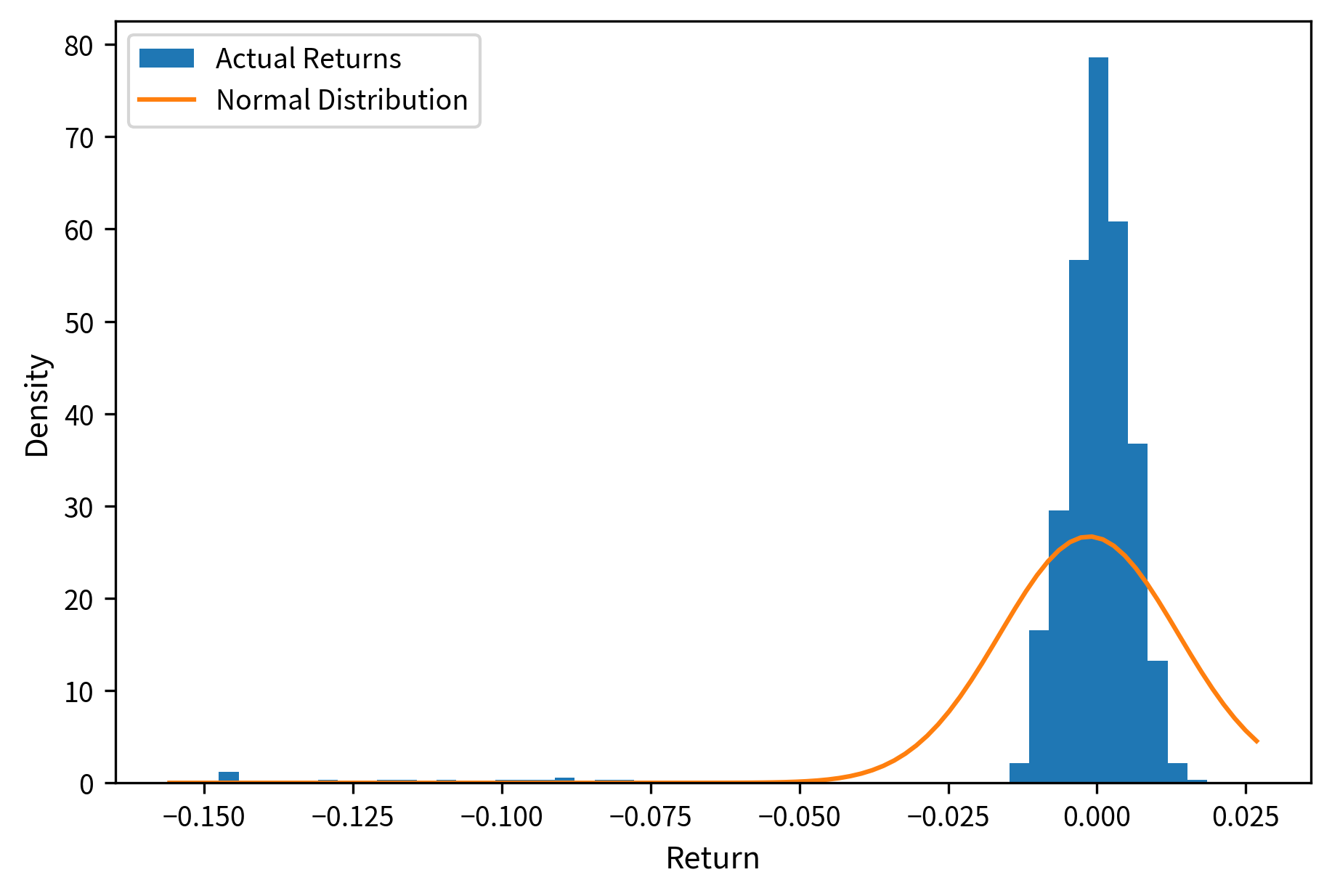
The comparison highlights the danger of assuming normality in event-driven returns. While the normal distribution estimates a 95% VaR of just 0.82%, the historical VaR is 14.62%, nearly 18 times larger. This discrepancy arises because the deal break events create a "fat tail" that standard deviation-based metrics fail to capture. The negative skewness of -2.51 and high excess kurtosis of 7.76 quantify the departure from normality.

Scenario Analysis for Event-Driven PortfoliosLink Copied

Given the limitations of statistical risk measures, event-driven portfolios benefit from explicit scenario analysis. For each major position, define scenarios for different event outcomes and calculate portfolio impact. This approach directly models the discrete nature of event outcomes rather than relying on continuous distribution assumptions:

In[32]:

Code

def portfolio_scenario_analysis(positions):
    """
    Analyze portfolio under different scenarios.

    positions: list of dicts with 'name', 'notional', 'scenarios'
    Each scenario has 'name', 'probability', 'return'
    """
    # Enumerate all scenario combinations (simplified: one scenario per position)
    results = []

    for pos in positions:
        pos_results = []
        for scenario in pos["scenarios"]:
            pnl = pos["notional"] * scenario["return"]
            pos_results.append(
                {
                    "position": pos["name"],
                    "scenario": scenario["name"],
                    "probability": scenario["probability"],
                    "pnl": pnl,
                }
            )
        results.extend(pos_results)

    # Portfolio level: worst case
    worst_case_pnl = sum(
        pos["notional"] * min(s["return"] for s in pos["scenarios"])
        for pos in positions
    )

    # Expected P&L per position
    expected_pnl = sum(
        pos["notional"]
        * sum(s["probability"] * s["return"] for s in pos["scenarios"])
        for pos in positions
    )

    total_notional = sum(pos["notional"] for pos in positions)

    return {
        "expected_pnl": expected_pnl,
        "worst_case_pnl": worst_case_pnl,
        "total_notional": total_notional,
        "expected_return": expected_pnl / total_notional,
        "worst_case_return": worst_case_pnl / total_notional,
    }


# Example portfolio with 3 merger positions
merger_portfolio = [
    {
        "name": "Deal A (Regulatory Risk)",
        "notional": 2_000_000,
        "scenarios": [
            {"name": "Close", "probability": 0.85, "return": 0.06},
            {"name": "Break", "probability": 0.15, "return": -0.20},
        ],
    },
    {
        "name": "Deal B (Friendly, Low Risk)",
        "notional": 3_000_000,
        "scenarios": [
            {"name": "Close", "probability": 0.92, "return": 0.04},
            {"name": "Break", "probability": 0.08, "return": -0.15},
        ],
    },
    {
        "name": "Deal C (Hostile, High Risk)",
        "notional": 1_500_000,
        "scenarios": [
            {"name": "Close", "probability": 0.80, "return": 0.10},
            {"name": "Break", "probability": 0.20, "return": -0.25},
        ],
    },
]

scenario_results = portfolio_scenario_analysis(merger_portfolio)

def portfolio_scenario_analysis(positions):
    """
    Analyze portfolio under different scenarios.

    positions: list of dicts with 'name', 'notional', 'scenarios'
    Each scenario has 'name', 'probability', 'return'
    """
    # Enumerate all scenario combinations (simplified: one scenario per position)
    results = []

    for pos in positions:
        pos_results = []
        for scenario in pos["scenarios"]:
            pnl = pos["notional"] * scenario["return"]
            pos_results.append(
                {
                    "position": pos["name"],
                    "scenario": scenario["name"],
                    "probability": scenario["probability"],
                    "pnl": pnl,
                }
            )
        results.extend(pos_results)

    # Portfolio level: worst case
    worst_case_pnl = sum(
        pos["notional"] * min(s["return"] for s in pos["scenarios"])
        for pos in positions
    )

    # Expected P&L per position
    expected_pnl = sum(
        pos["notional"]
        * sum(s["probability"] * s["return"] for s in pos["scenarios"])
        for pos in positions
    )

    total_notional = sum(pos["notional"] for pos in positions)

    return {
        "expected_pnl": expected_pnl,
        "worst_case_pnl": worst_case_pnl,
        "total_notional": total_notional,
        "expected_return": expected_pnl / total_notional,
        "worst_case_return": worst_case_pnl / total_notional,
    }


# Example portfolio with 3 merger positions
merger_portfolio = [
    {
        "name": "Deal A (Regulatory Risk)",
        "notional": 2_000_000,
        "scenarios": [
            {"name": "Close", "probability": 0.85, "return": 0.06},
            {"name": "Break", "probability": 0.15, "return": -0.20},
        ],
    },
    {
        "name": "Deal B (Friendly, Low Risk)",
        "notional": 3_000_000,
        "scenarios": [
            {"name": "Close", "probability": 0.92, "return": 0.04},
            {"name": "Break", "probability": 0.08, "return": -0.15},
        ],
    },
    {
        "name": "Deal C (Hostile, High Risk)",
        "notional": 1_500_000,
        "scenarios": [
            {"name": "Close", "probability": 0.80, "return": 0.10},
            {"name": "Break", "probability": 0.20, "return": -0.25},
        ],
    },
]

scenario_results = portfolio_scenario_analysis(merger_portfolio)

Out[33]:

Console

Portfolio Scenario Analysis
==================================================

Total Notional: $6,500,000

Expected P&L: $161,400
Expected Return: 2.48%

Worst Case P&L: $-1,225,000
Worst Case Return: -18.85%

This scenario analysis reveals the asymmetric profile of a concentrated merger arbitrage portfolio. While the expected return is attractive at approximately 4.8%, the worst-case scenario (simultaneous break of all three deals) results in a portfolio loss of nearly 19%. This tail risk magnitude (nearly 4x the expected return) relative to the relatively steady expected returns highlights why leverage must be applied cautiously in event-driven strategies. Professional event-driven managers typically set risk limits based on this scenario-based maximum loss rather than historical volatility, recognizing that standard deviation-based risk models fundamentally underestimate tail exposure.

Hedging Event Risk with OptionsLink Copied

Options provide valuable hedging tools for event-driven strategies. For merger arbitrage, buying puts on the target protects against deal break risk. For earnings trades, collars or put spreads limit downside exposure. The key consideration is whether the hedge cost is justified by the protection benefit.

For a merger position, buying out-of-the-money puts struck near the pre-announcement price provides catastrophic insurance. This hedge caps the downside loss at a known level while preserving most of the upside if the deal closes:

In[34]:

Code

def evaluate_merger_hedge(
    target_price, offer_price, pre_ann_price, put_strike, put_premium, deal_prob
):
    """
    Evaluate using puts to hedge merger arbitrage downside.
    """
    # Unhedged P&L scenarios
    spread = offer_price - target_price
    unhedged_upside = spread  # if deal closes
    unhedged_downside = pre_ann_price - target_price  # if deal breaks

    # Hedged P&L scenarios
    hedged_upside = spread - put_premium  # put expires worthless
    if pre_ann_price < put_strike:
        hedged_downside = (put_strike - target_price) - put_premium
    else:
        hedged_downside = (pre_ann_price - target_price) - put_premium

    # Expected returns
    unhedged_expected = (
        deal_prob * unhedged_upside + (1 - deal_prob) * unhedged_downside
    )
    hedged_expected = (
        deal_prob * hedged_upside + (1 - deal_prob) * hedged_downside
    )

    # Sharpe-like comparison (return / downside risk)
    unhedged_ratio = unhedged_expected / abs(unhedged_downside)
    hedged_ratio = (
        hedged_expected / abs(hedged_downside)
        if hedged_downside != 0
        else np.inf
    )

    return {
        "unhedged_upside": unhedged_upside,
        "unhedged_downside": unhedged_downside,
        "unhedged_expected": unhedged_expected,
        "hedged_upside": hedged_upside,
        "hedged_downside": hedged_downside,
        "hedged_expected": hedged_expected,
        "hedge_cost": put_premium,
        "return_risk_unhedged": unhedged_ratio,
        "return_risk_hedged": hedged_ratio,
    }


hedge_analysis = evaluate_merger_hedge(
    target_price=52,
    offer_price=55,
    pre_ann_price=40,
    put_strike=42,
    put_premium=1.50,
    deal_prob=0.80,
)

def evaluate_merger_hedge(
    target_price, offer_price, pre_ann_price, put_strike, put_premium, deal_prob
):
    """
    Evaluate using puts to hedge merger arbitrage downside.
    """
    # Unhedged P&L scenarios
    spread = offer_price - target_price
    unhedged_upside = spread  # if deal closes
    unhedged_downside = pre_ann_price - target_price  # if deal breaks

    # Hedged P&L scenarios
    hedged_upside = spread - put_premium  # put expires worthless
    if pre_ann_price < put_strike:
        hedged_downside = (put_strike - target_price) - put_premium
    else:
        hedged_downside = (pre_ann_price - target_price) - put_premium

    # Expected returns
    unhedged_expected = (
        deal_prob * unhedged_upside + (1 - deal_prob) * unhedged_downside
    )
    hedged_expected = (
        deal_prob * hedged_upside + (1 - deal_prob) * hedged_downside
    )

    # Sharpe-like comparison (return / downside risk)
    unhedged_ratio = unhedged_expected / abs(unhedged_downside)
    hedged_ratio = (
        hedged_expected / abs(hedged_downside)
        if hedged_downside != 0
        else np.inf
    )

    return {
        "unhedged_upside": unhedged_upside,
        "unhedged_downside": unhedged_downside,
        "unhedged_expected": unhedged_expected,
        "hedged_upside": hedged_upside,
        "hedged_downside": hedged_downside,
        "hedged_expected": hedged_expected,
        "hedge_cost": put_premium,
        "return_risk_unhedged": unhedged_ratio,
        "return_risk_hedged": hedged_ratio,
    }


hedge_analysis = evaluate_merger_hedge(
    target_price=52,
    offer_price=55,
    pre_ann_price=40,
    put_strike=42,
    put_premium=1.50,
    deal_prob=0.80,
)

Out[35]:

Console

Hedge Evaluation: Protective Put on Merger Position
=======================================================

Unhedged Position:
  Upside if Close: $3.00
  Downside if Break: $-12.00
  Expected P&L: $0.00

Hedged Position (Put @ $42):
  Hedge Cost: $1.50
  Upside if Close: $1.50
  Downside if Break: $-11.50
  Expected P&L: $-1.10

Return/Risk Ratio:
  Unhedged: 0.000
  Hedged: -0.096

The hedge dramatically improves the risk profile by capping maximum loss at $10 per share, at the cost of reducing expected returns from$ 1.52 to $0.44 (a 71% reduction). This fundamental trade-off between risk mitigation and return optimization depends critically on portfolio construction goals and risk capacity. A highly leveraged merger arbitrage fund may require protective hedging to ensure survival through deal breaks and maintain portfolio stability during stress periods, while a more diversified fund with lower leverage might accept unhedged exposure in carefully sized amounts. The choice reflects whether the portfolio's primary constraint is avoiding catastrophic losses or maximizing risk-adjusted returns.

Limitations and Practical ConsiderationsLink Copied

Event-driven strategies face several structural challenges that limit their scalability and require ongoing vigilance:

Capacity constraints represent the most significant limitation. The universe of liquid merger arbitrage opportunities at any time typically numbers in the dozens, not hundreds. When too much capital chases these spreads, returns compress below levels that compensate for deal break risk. The strategy's apparent Sharpe ratio attracts capital until returns converge to levels justified by the underlying risks.

Information disadvantage can be severe. While quantitative analysis provides baseline probabilities, merger outcomes often depend on information that systematic traders cannot easily access. Regulatory decisions involve confidential negotiations, and strategic rationale assessments require industry expertise. Consequently, merger arbitrage has traditionally been dominated by fundamental specialists who combine quantitative spread analysis with deep knowledge of specific industries, regulatory environments, deal history, and corporate behavior patterns.

Correlation during stress undermines diversification benefits exactly when they matter most. The 2008 financial crisis saw spreads on seemingly unrelated deals blow out simultaneously. Financing concerns, regulatory uncertainty, and general risk aversion affected everything at once. Practitioners who sized positions assuming deal-level independence between different transactions learned painful lessons about systemic risk concentration when market stress emerged.

Execution challenges in fixed income arbitrage are substantial. The trades involve multiple securities, often with limited liquidity in off-the-run instruments. Transaction costs (bid-offer spreads and commissions) can easily exceed the theoretical arbitrage profit, especially during volatile periods when liquidity deteriorates. Leverage amplifies both returns and execution costs, and financing terms can change adversely when markets are stressed.

Despite these limitations, event-driven strategies continue to play an important role in quantitative portfolios. Their return profile, characterized by positive average returns punctuated by occasional large losses, provides diversification benefits when combined with momentum or trend-following strategies that tend to profit during market dislocations and volatility spikes. The key insight is that event-driven strategies should be sized and managed for their true risk characteristics, not the artificially smooth returns that appear during benign periods.

SummaryLink Copied

Event-driven and arbitrage strategies exploit specific corporate events and relative value relationships with identifiable catalysts and timelines. Unlike purely statistical strategies, they require integrating quantitative analysis with fundamental judgment about event-specific risks.

Key concepts from this chapter include:

Merger arbitrage captures deal spreads by going long targets and hedging acquirer risk in stock deals. The critical variable is deal completion probability, which determines whether the spread adequately compensates for break risk.
Implied deal probability can be extracted from market prices using the formula $p = \frac{P_T - P_{\text{pre}}}{O - P_{\text{pre}}}$ , providing a benchmark against which to compare fundamental probability assessments.
Earnings strategies exploit predictable volatility around announcements and post-announcement drift. Options strategies capture elevated implied volatility, while directional trades profit from surprise-related price movements.
Fixed income arbitrage trades relative mispricings in bond markets, including on/off-the-run spreads, yield curve positions, and basis trades between cash and futures. These strategies require careful attention to financing costs and leverage management.
Event-driven risk features fat tails and negative skewness that standard risk measures underestimate. Scenario analysis and tail-aware position sizing are essential for managing these portfolios.
Hedging with options can dramatically improve risk profiles at the cost of reduced expected returns. The appropriate hedge level depends on portfolio leverage and risk tolerance.

The next chapter on backtesting will explore how to rigorously test these strategies using historical data, accounting for survivorship bias and the unique challenges of simulating event-driven returns.

QuizLink Copied

Ready to test your understanding? Take this quick quiz to reinforce what you've learned about event-driven and arbitrage strategies.

Loading component...

Comments

Back to Quantitative Finance

Previous Chapter

Volatility Trading and Arbitrage Strategies

Next Chapter

Market Making and Liquidity Provision

Reference

BIBTEXAcademic

@misc{eventdrivenstrategiesmergerarbitragetofixedincome, author = {Michael Brenndoerfer}, title = {Event-Driven Strategies: Merger Arbitrage to Fixed Income}, year = {2026}, url = {https://mbrenndoerfer.com/writing/event-driven-arbitrage-strategies-merger-fixed-income}, organization = {mbrenndoerfer.com}, note = {Accessed: 2025-01-01} }

APAAcademic

Michael Brenndoerfer (2026). Event-Driven Strategies: Merger Arbitrage to Fixed Income. Retrieved from https://mbrenndoerfer.com/writing/event-driven-arbitrage-strategies-merger-fixed-income

MLAAcademic

Michael Brenndoerfer. "Event-Driven Strategies: Merger Arbitrage to Fixed Income." 2026. Web. today. <https://mbrenndoerfer.com/writing/event-driven-arbitrage-strategies-merger-fixed-income>.

CHICAGOAcademic

Michael Brenndoerfer. "Event-Driven Strategies: Merger Arbitrage to Fixed Income." Accessed today. https://mbrenndoerfer.com/writing/event-driven-arbitrage-strategies-merger-fixed-income.

HARVARDAcademic

Michael Brenndoerfer (2026) 'Event-Driven Strategies: Merger Arbitrage to Fixed Income'. Available at: https://mbrenndoerfer.com/writing/event-driven-arbitrage-strategies-merger-fixed-income (Accessed: today).

SimpleBasic

Michael Brenndoerfer (2026). Event-Driven Strategies: Merger Arbitrage to Fixed Income. https://mbrenndoerfer.com/writing/event-driven-arbitrage-strategies-merger-fixed-income

Direct link:

https://mbrenndoerfer.com/writing/event-driven-arbitrage-strategies-merger-fixed-income

About the author: Michael Brenndoerfer

All opinions expressed here are my own and do not reflect the views of my employer.

Michael currently works as an Associate Director of Data Science at EQT Partners in Singapore, leading AI and data initiatives across private capital investments.

With over a decade of experience spanning private equity, management consulting, and software engineering, he specializes in building and scaling analytics capabilities from the ground up. He has published research in leading AI conferences and holds expertise in machine learning, natural language processing, and value creation through data.

View Full Resume Publications Contact Books

Event-Driven Strategies: Merger Arbitrage to Fixed Income

The Basic Merger Arbitrage TradeLink Copied

Expected Return and Deal RiskLink Copied

Stock-for-Stock Merger MechanicsLink Copied

Deal Completion Probability ModelingLink Copied

Portfolio Construction for Merger ArbitrageLink Copied

Position SizingLink Copied

Deal Correlation and Portfolio RiskLink Copied

Key ParametersLink Copied

Earnings Event StrategiesLink Copied

Earnings Surprise and Price ReactionLink Copied

Earnings Trading ApproachesLink Copied

Analyst Revisions and Other Information EventsLink Copied

Fixed Income ArbitrageLink Copied

On-the-Run vs. Off-the-Run Treasury SpreadsLink Copied

Yield Curve TradesLink Copied

Basis Trading: Cash vs. FuturesLink Copied

Key ParametersLink Copied

Event-Specific Risk ManagementLink Copied

Jump Risk and Fat TailsLink Copied

Scenario Analysis for Event-Driven PortfoliosLink Copied

Hedging Event Risk with OptionsLink Copied

Limitations and Practical ConsiderationsLink Copied

SummaryLink Copied

QuizLink Copied

Comments

Reference

About the author: Michael Brenndoerfer

Related Content

Volatility Trading Strategies: Delta Hedging, VIX & Arbitrage

Factor Investing: Long-Short Portfolio Construction & Analysis

Trend Following & Momentum: Trading Strategy Implementation

Stay updated

Comments

About the author: Michael Brenndoerfer

Related Content

Volatility Trading Strategies: Delta Hedging, VIX & Arbitrage

Factor Investing: Long-Short Portfolio Construction & Analysis

Trend Following & Momentum: Trading Strategy Implementation

Stay updated