

Learn how market makers profit from bid-ask spreads while managing inventory risk. Explore the Avellaneda-Stoikov model for optimal quote placement.
Choose your expertise level to adjust how many terms are explained. Beginners see more tooltips, experts see fewer to maintain reading flow. Hover over underlined terms for instant definitions.
Market Making and Liquidity Provision
Financial markets require participants willing to stand ready to buy and sell at any moment. You fulfill this essential role by continuously posting bid and ask quotes, providing liquidity to traders who need immediate execution. In exchange for this service, you capture the bid-ask spread, the difference between the price at which you buy and the price at which you sell.
Modern market making has evolved from human specialists on exchange floors to sophisticated algorithmic systems that quote across thousands of instruments simultaneously. You use mathematical models to determine optimal quote placement, manage inventory risk, and protect against informed traders. The business model is deceptively simple: buy at the bid, sell at the ask, pocket the spread. But the execution is extraordinarily complex, requiring real-time risk management, microsecond-level technology, and deep understanding of market dynamics.
This chapter explores the economics of market making, the mathematical models that guide quoting decisions, and the key risks you face. We will build a simulation framework to understand how these strategies work in practice and examine why speed and risk management are critical to success.
The Economics of Market Making
You profit by providing a service: immediacy. When a trader wants to buy a stock right now, they don't want to wait for another natural seller to appear. You offer to sell immediately, but at a premium, the ask price. Similarly, when someone wants to sell immediately, you buy at the bid price, which is lower than fair value. This willingness to take the other side of any trade, at any time, is what makes markets function smoothly. Without market makers, traders would face significant delays finding counterparties, and the uncertainty of execution timing would itself become a substantial cost of trading.
The bid-ask spread is the difference between the highest price a buyer is willing to pay (the bid) and the lowest price a seller is willing to accept (the ask). You earn this spread by buying at the bid and selling at the ask.
Consider a simple example that illustrates the core economics. You quote a stock with a bid of 100.05. The spread is $0.10. If you buy 100 shares at the bid and sell 100 shares at the ask, the gross profit is:
This calculation is simple. However, several practical complications transform it into an optimization problem:
- Inventory accumulation: Trades don't arrive in perfect alternation. You might buy 500 shares before selling any, accumulating inventory that could lose value if prices move against you. This imbalance is the norm. Order flow is unpredictable, often leading to unintended positions.
- Adverse selection: Some traders have better information about future prices. When an informed trader buys, it often signals that prices will rise, meaning you just sold too cheaply. This information asymmetry is a serious risk in market making because it systematically transfers wealth from you to informed traders.
- Competition: Competition for order flow compresses spreads. In liquid markets, even small inefficiencies can eliminate profit.
- Volatility: Higher volatility means greater risk of price moves between when you buy and sell. A position held for even a few seconds during a volatile period can experience significant adverse price movement.
Understanding these factors allows us to express your expected profit per single trade in a more complete form:
where:
- : bid-ask spread
- Adverse Selection Cost: expected loss to informed traders
- Inventory Cost: cost of holding inventory risk
The factor of appears because you earn half the spread on each side of a trade relative to the mid price. To understand why this is the case, consider that the mid price represents the market's best estimate of fair value. When you buy at the bid, you pay a price that is below the mid price. When you sell at the ask, you receive a price that is above the mid price. Each individual trade therefore generates revenue of half the spread relative to fair value. Successful market making requires setting spreads wide enough to cover adverse selection and inventory costs while remaining competitive enough to attract order flow. This delicate balance defines the central challenge of the market making business.
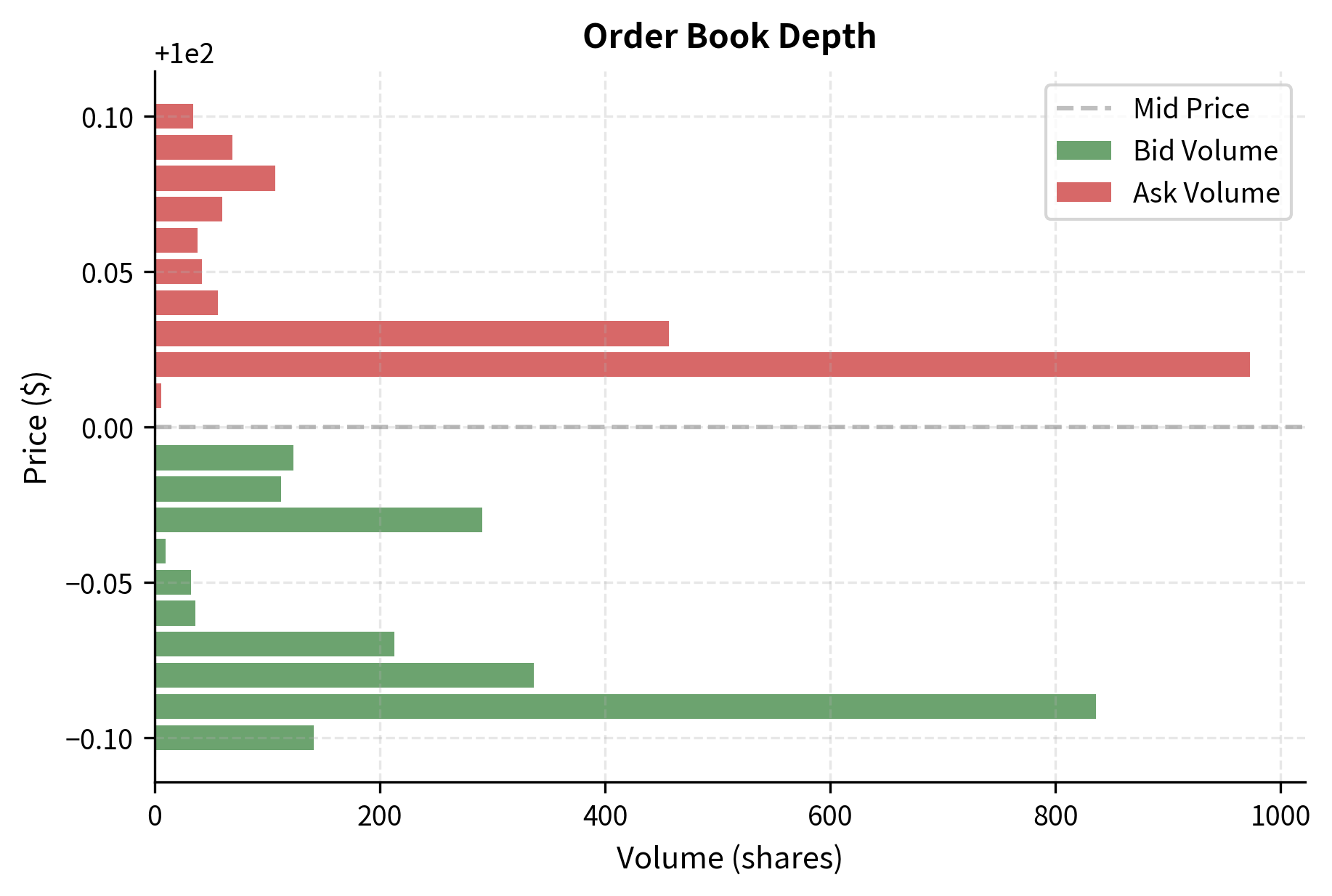
Order Book Mechanics
To understand market making, you need to understand the limit order book, the fundamental data structure that organizes trading in modern electronic markets. As we'll explore in more detail in the upcoming chapter on Market Microstructure, the order book aggregates all outstanding buy and sell orders at various price levels. Think of the order book as a ledger that records every participant's willingness to trade at specific prices, continuously updated as orders arrive, execute, or are cancelled.
A limit order book is an electronic record of all outstanding orders to buy or sell a security at specific prices. Buy orders (bids) are sorted from highest to lowest price, while sell orders (asks) are sorted from lowest to highest.
There are two primary order types that interact with this book structure:
- Limit orders specify a maximum price (for buys) or minimum price (for sells) and wait in the book until matched. You primarily use limit orders to post your quotes. These orders provide liquidity to the market: they sit passively in the book, waiting for someone else to trade against them. You don't know when or if your order will execute, but you do know the price you will receive if it does.
- Market orders execute immediately against the best available limit orders in the book. Traders demanding immediacy use market orders. These orders consume liquidity: they remove resting limit orders from the book. The market order submitter knows their order will execute immediately, but they don't control the exact price they will receive.
The order book shows the best bid at 100.01, creating a spread of $0.02. When you post at the inside (best bid and ask), your quote has priority over orders further from the mid price. This priority is crucial because orders at the same price typically execute in time priority, meaning the first order to arrive at a given price level executes first. When a market buy order arrives, it executes against the best ask; a market sell order executes against the best bid. This matching process continues until the incoming order is fully filled or the book is exhausted at that price level.
You must decide at which price levels to place your orders and how much size to offer. This decision involves a fundamental trade-off that shapes all market making strategies. Posting at the inside quote provides the highest probability of execution but the smallest profit per trade. Posting further from the mid price increases profit per trade but reduces execution probability. The optimal choice depends on many factors, including the volatility of the asset, the behavior of other market participants, and your current inventory position.
Inventory Risk
The central challenge in market making is inventory risk, the risk that accumulated positions will lose value before they can be unwound. If you buy more than you sell, you accumulate a long position. If prices then fall, you suffer losses that may exceed the spread revenue earned. This risk is unavoidable because you cannot control the timing or direction of incoming orders. You must quote continuously, but you cannot determine which of your quotes will be executed.
The Inventory Accumulation Problem
Consider a scenario where you start the day flat (no position). Over the course of trading, order arrivals are random. Sometimes more buyers arrive, causing you to sell and become short. Other times more sellers arrive, causing you to buy and become long. Your inventory thus evolves as a consequence of the random sequence of order arrivals, not as a result of any deliberate trading decision.
We can model inventory evolution as a random process. This mathematical framework helps us understand why inventory accumulation is such a persistent concern. Let denote your inventory at time . Each trade changes inventory by (assuming unit trade sizes):
where:
- : current inventory level
- : change in inventory (+1 for buy, -1 for sell)
- : inventory level after the trade
If a market sell order arrives, you buy (). If a market buy order arrives, you sell (). Notice that you take the opposite side of each incoming order, which is what it means to "make a market." The inventory change is thus determined by the arriving order, not by your preference.
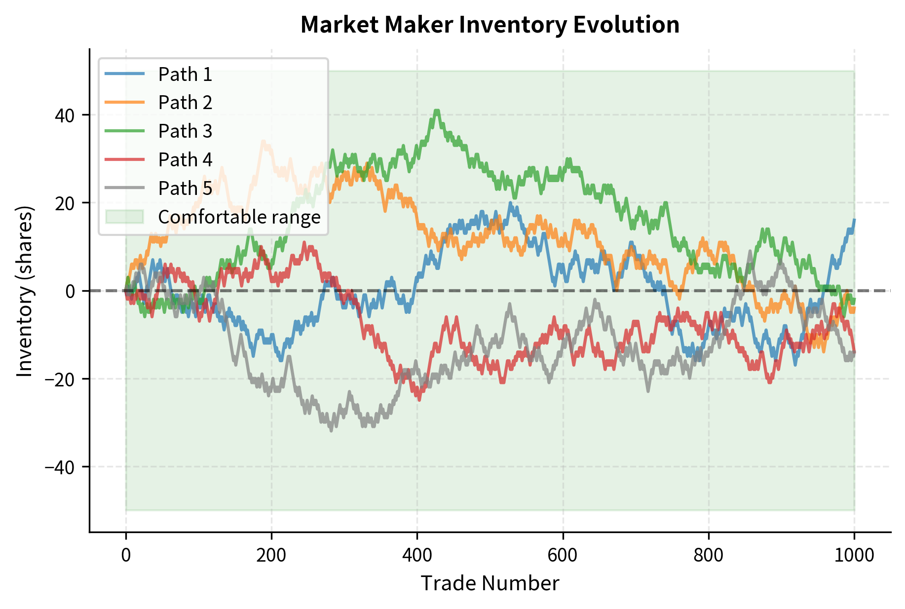
The simulation reveals a crucial insight about market making dynamics. Even with perfectly balanced order flow, where buys and sells arrive with equal probability, inventory follows a random walk and can drift far from zero. This is a mathematical consequence of the random walk properties: the expected position is zero, but the variance of the position grows with the number of trades. This drift is dangerous because it exposes you to directional price risk, exactly the risk you don't want to take. You aim to profit from the spread, not from predicting price direction. Yet without active management, you inevitably accumulate positions that bet on price direction.
Quantifying Inventory Risk
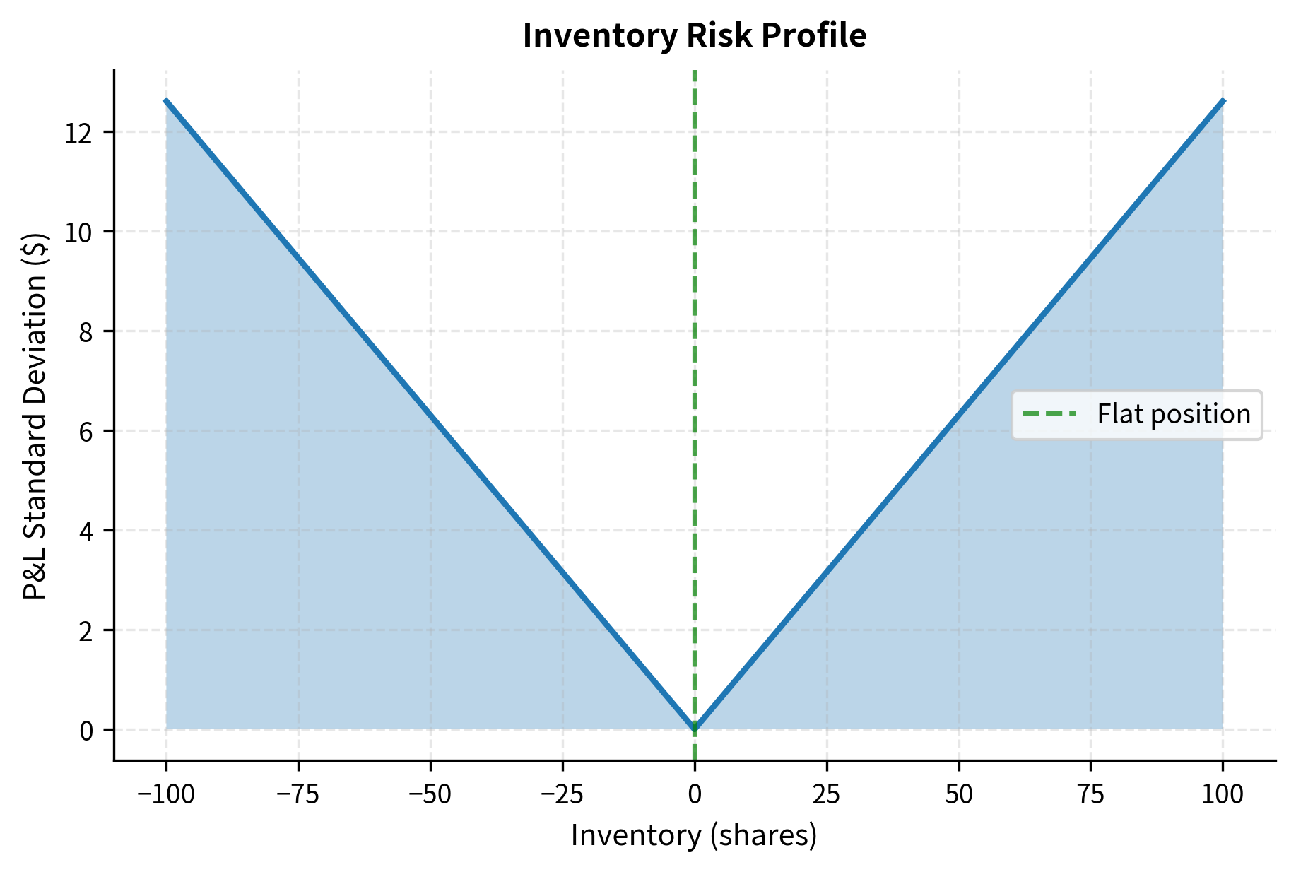
To understand how to manage inventory risk, we must first quantify it precisely. The P&L impact of inventory comes from price changes. If you hold inventory and the price changes by , the inventory P&L is:
where:
- : current inventory position
- : change in asset price
This formula captures the essence of the risk: your profit or loss depends on how much inventory you hold and how much the price moves. A long position profits when prices rise and loses when prices fall; a short position has the opposite exposure.
The variance of inventory P&L over a short time interval can be derived from the price variance. This derivation connects our understanding of price dynamics to the specific risk you face. Assuming the asset price follows a random walk with percentage volatility :
where:
- : inventory size
- : change in asset price
- : current asset price
- : annualized volatility (percentage)
- : time interval
This result reveals a critical insight: inventory risk grows quadratically with position size. Holding twice the inventory creates four times the variance, not twice the variance. This non-linear relationship means that large positions are disproportionately risky. If you hold 100 shares, you face four times the risk variance of holding 50 shares, even though you hold only twice as many shares. This quadratic scaling provides strong incentive to keep positions small.
This risk profile motivates a key market making principle: inventory mean reversion. You should actively adjust your quotes to encourage trades that reduce inventory. When long, you lower your ask price to attract buyers; when short, you raise your bid price to attract sellers. This quote adjustment technique is called "skewing" and represents the primary tool you use to control their exposure. By making it more attractive for the market to trade in the direction that reduces your position, you can systematically pull your inventory back toward zero without waiting passively for favorable order flow.
Adverse Selection
Beyond inventory risk, you face adverse selection, the risk of trading against informed counterparties who know more about future prices than you do. This concept, which we touched on in our discussion of liquidity risk Part V, is fundamental to understanding why market making spreads exist. While inventory risk can be managed through quote adjustment and hedging, adverse selection represents a more insidious challenge because it systematically extracts value from you.
Information Asymmetry
Consider the market for a stock about to report earnings. Some traders may have superior analysis or even inside information about the announcement. When these informed traders buy, it signals that the stock is likely undervalued, meaning you are selling too cheaply. When informed traders sell, you are buying something that will soon be worth less. You cannot distinguish between informed and uninformed traders at the moment of the trade; you only discover afterward, when prices move, whether your counterparty was informed.
Adverse selection occurs when one party to a transaction has information that the other lacks. In market making, informed traders profit at your expense by trading when they have superior knowledge of future price movements.
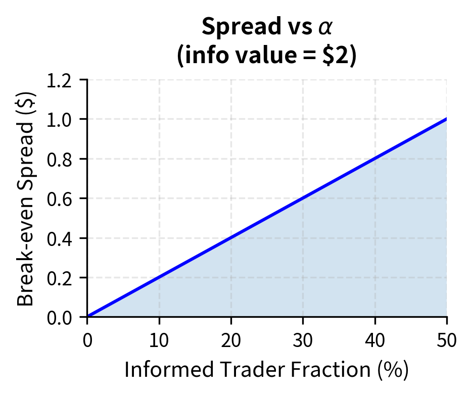
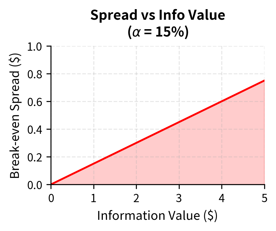
The famous Glosten-Milgrom model formalizes this intuition, providing a theoretical foundation for understanding how adverse selection affects market making. Suppose a fraction of traders are informed and know the true value of the asset, while the remaining are uninformed liquidity traders who trade for reasons unrelated to the asset's fundamental value. You must set quotes knowing that:
- When an informed trader buys, (you sold too cheaply)
- When an informed trader sells, (you bought too expensively)
- Uninformed traders buy and sell randomly
The key insight is that you face a winner's curse problem. You are more likely to execute trades precisely when those trades are unfavorable. Informed traders only trade when your quotes are mispriced relative to true value, while uninformed traders provide a mixture of profitable and unprofitable trades. Your break-even spread must compensate for losses to informed traders:
where:
- : break-even spread
- : probability that the next trader is informed
- : difference between the asset's high and low values (value of private information)
Higher informed trading probability requires wider spreads to compensate for the greater expected losses to informed counterparties. Similarly, when the value of private information is larger (the gap between and is greater), spreads must widen because each trade against an informed counterparty generates larger losses.
Detecting Informed Flow
You use various signals to detect potentially informed order flow. These detection methods are imperfect, but they can help you adjust your quotes or trade sizes when the risk of adverse selection appears elevated:
- Order size: Large orders may signal informed trading because informed traders have greater incentive to trade large quantities when they possess valuable information
- Order timing: Trades just before news announcements are more likely to be informed, as traders may have advance knowledge or superior forecasting ability
- Order toxicity: Metrics like VPIN (Volume-synchronized Probability of Informed Trading) attempt to measure the proportion of informed flow in real time
- Price impact: Orders that move prices significantly suggest the market is updating its beliefs in response to perceived information content
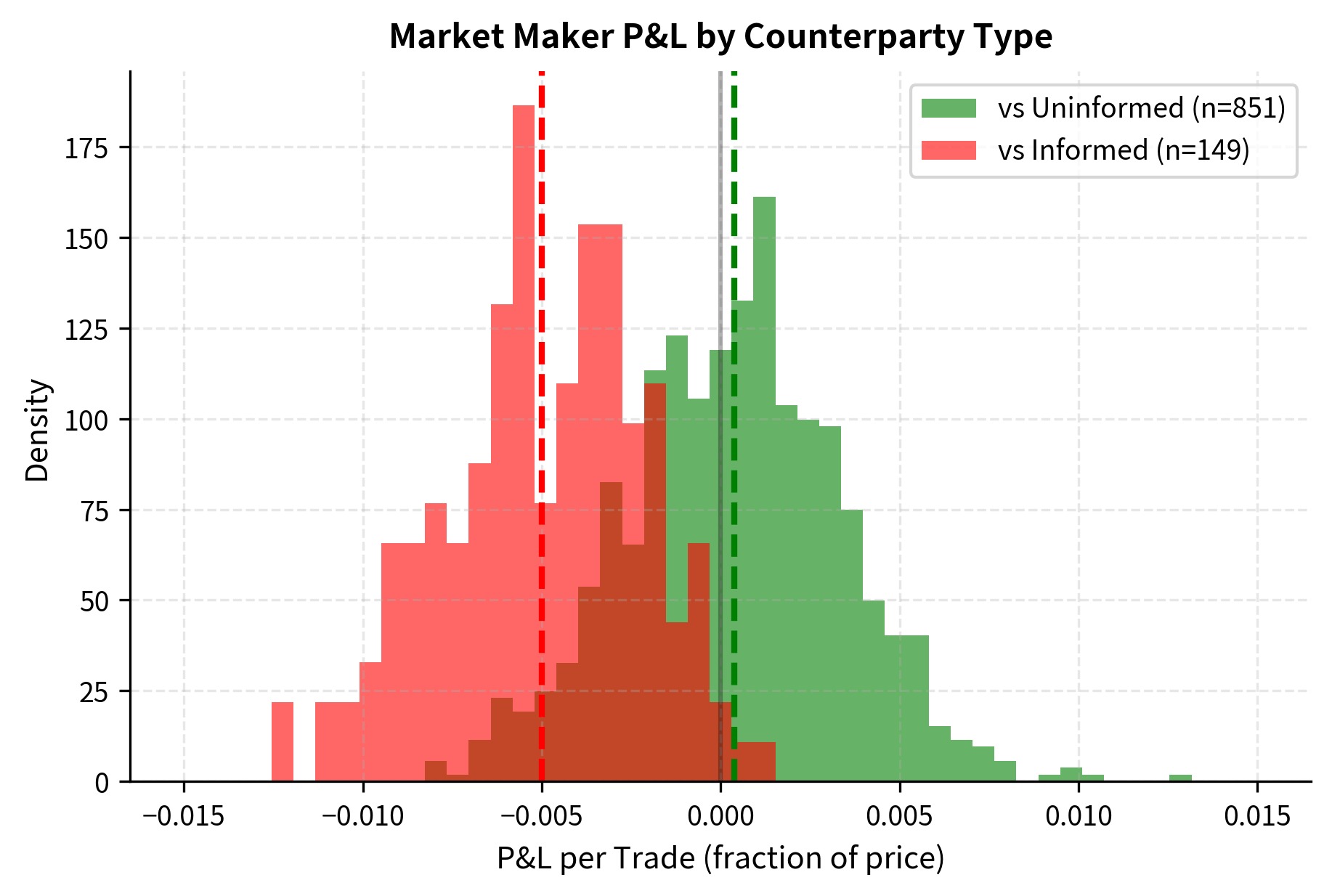
The simulation clearly shows the adverse selection problem in action. We earn money against uninformed traders but lose even more against informed traders. The overall P&L depends critically on the fraction of informed flow and the size of the information edge. This is why you should obsess over order flow quality: a venue or counterparty that generates predominantly uninformed flow is enormously valuable, while flow with high informed content can quickly destroy profitability.
Optimal Market Making: The Avellaneda-Stoikov Model
The foundational quantitative model for market making was developed by Marco Avellaneda and Sasha Stoikov in 2008. This model provides optimal bid and ask quotes that balance the trade-off between earning spread and managing inventory risk. The model produces closed-form solutions that capture the essential economics of market making while remaining tractable enough for real-time implementation.
Model Setup
The Avellaneda-Stoikov model builds on several key assumptions that simplify the market making problem while preserving its essential features:
- The asset price follows arithmetic Brownian motion:
- You have a terminal time horizon and seek to maximize expected utility of terminal wealth
- Order arrivals follow Poisson processes with intensity depending on quote distance from mid price
- You have exponential utility with risk aversion parameter
Each assumption serves a specific purpose. Arithmetic Brownian motion simplifies the analysis while capturing the essential feature that prices fluctuate unpredictably. The terminal horizon reflects the fact that you cannot hold positions indefinitely and must eventually flatten your books. The Poisson arrival process captures the random nature of order flow, while exponential utility provides a tractable way to model risk aversion.
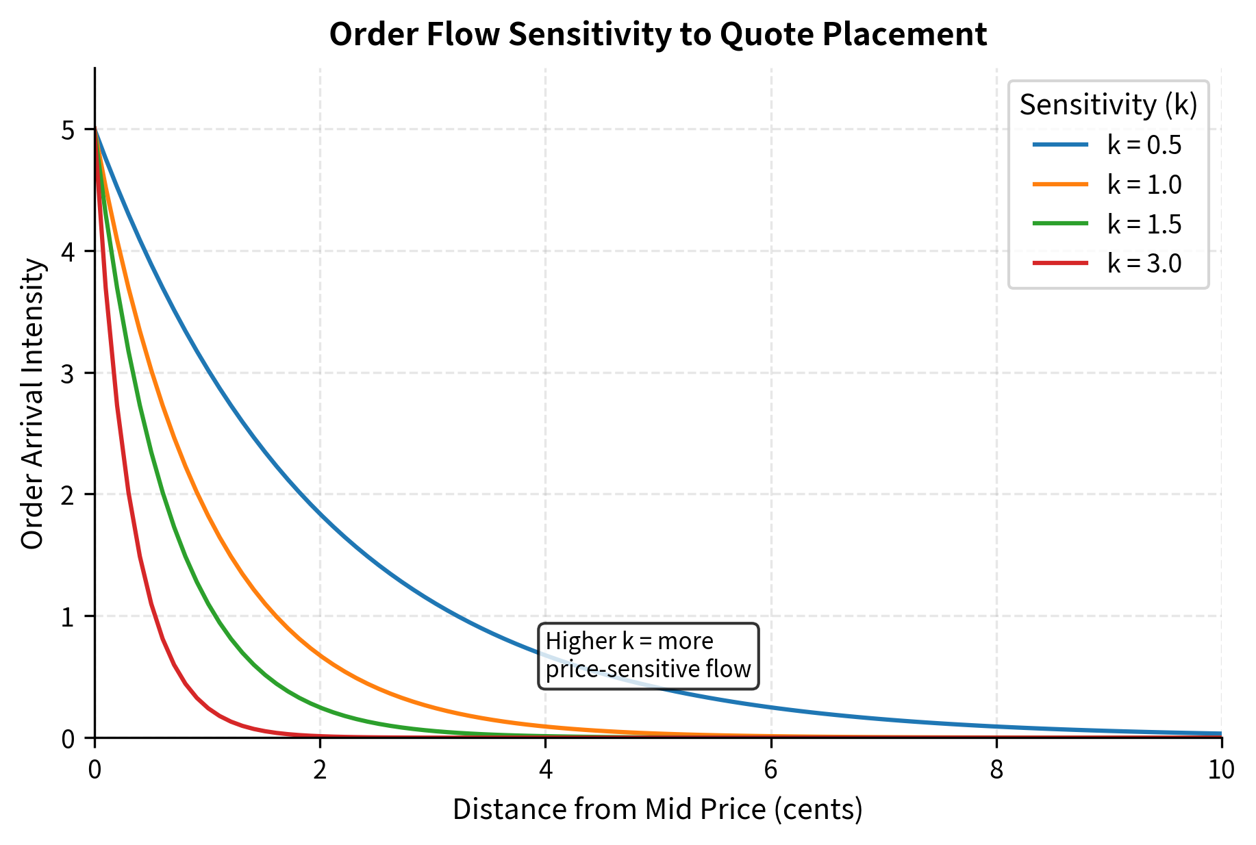
Let and be the distances of the ask and bid from the mid price. The order arrival intensity (rate) at a distance from the mid price is modeled as:
where:
- : arrival intensity
- : distance from mid price
- : baseline arrival rate
- : order flow sensitivity to price
This exponential decay function captures the fundamental trade-off in limit order trading: increasing the spread (larger ) yields more profit per trade but exponentially reduces the probability of execution. The parameter controls how sensitive order flow is to price. A high value of means that traders are very price-sensitive, so moving quotes even slightly away from the mid price dramatically reduces execution probability. A low value of indicates price-insensitive traders who will trade across a wider range of prices. Understanding the value of in a particular market is crucial for calibrating the model.
Optimal Quotes
The model yields closed-form optimal quotes through a dynamic programming argument. In this model, you maximize expected utility of terminal wealth, accounting for the uncertain arrival of orders and the risk of holding inventory. The solution introduces a fundamental concept called the reservation price, which represents your private valuation accounting for inventory:
where:
- : reservation price
- : current mid price
- : current inventory
- : risk aversion parameter
- : absolute volatility of the asset (in price units, distinct from percentage volatility)
- : time remaining until the terminal horizon
The key insight is that the reservation price shifts away from the mid price based on inventory. This shift quantifies how your risk changes your perception of fair value:
- When long (), the reservation price is below the mid price, encouraging selling
- When short (), the reservation price is above the mid price, encouraging buying
To understand why this makes sense, consider being long 50 shares. You face the risk that prices will fall, causing you to lose money on your position. From your perspective, a "fair" price for buying more shares is lower than the market mid price because additional purchases increase your risk. Conversely, a fair price for selling is also lower than the mid price because you are eager to reduce your risk exposure. The reservation price formula captures this adjustment precisely.
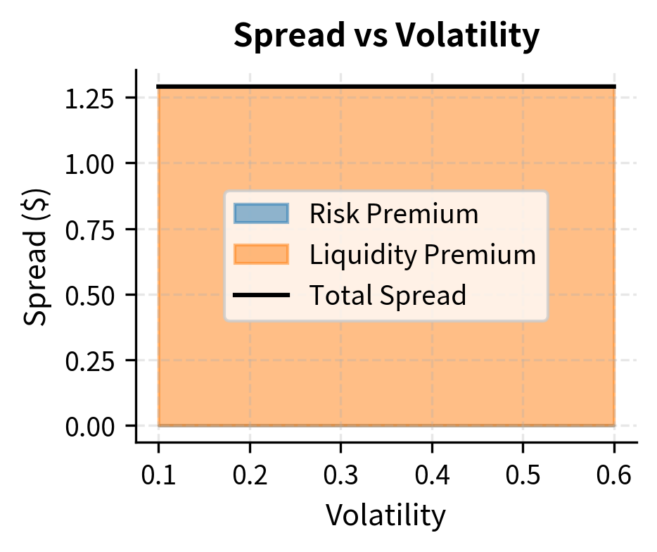
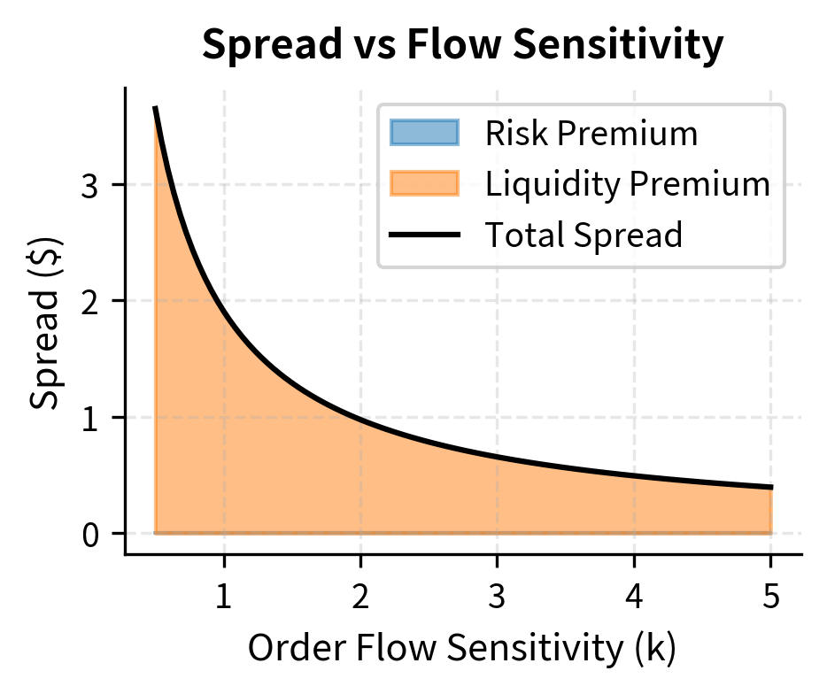
The optimal spread around this reservation price is:
where:
- : optimal spread
- : risk aversion parameter
- : absolute volatility
- : time remaining
- : order flow sensitivity
The spread consists of two terms, each with a distinct economic interpretation:
-
: a risk premium that widens with volatility and time horizon. This term reflects the inventory risk component. Higher volatility means greater potential for adverse price moves while holding inventory, so you demand a wider spread as compensation. Similarly, a longer time horizon means more time during which prices could move adversely.
-
: a liquidity premium driven by the elasticity of order flow (). This term captures the trade-off between profit per trade and execution probability. When order flow is very price-sensitive (high ), this term is small because you cannot afford to quote wide spreads without losing all your order flow. When order flow is price-insensitive (low ), you can extract larger spreads.
This leads to optimal bid and ask prices:
where:
- : optimal bid and ask quotes
- : reservation price
- : optimal spread
- : current mid price
- : current inventory
- : risk aversion parameter
- : absolute volatility
- : time remaining until horizon
These formulas show that both the bid and ask prices shift together based on inventory. The spread between them remains constant at , but the center of that spread, the reservation price, moves to encourage inventory-reducing trades.
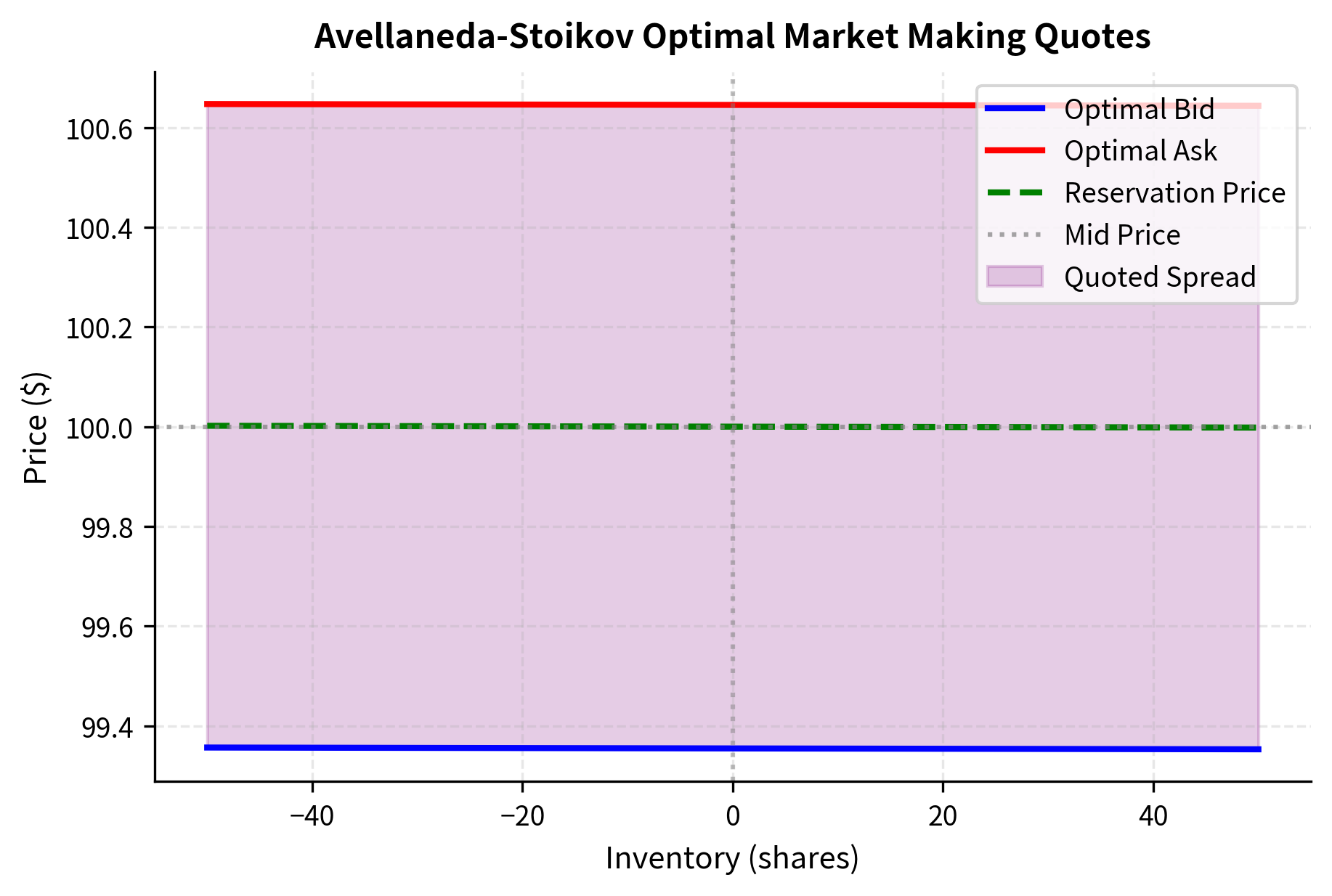
The figure shows the core intuition of inventory-based quoting. When you are flat (inventory = 0), quotes are centered around the mid price. As inventory grows positive (long position), both quotes shift down to encourage buying from you. The reservation price, what you consider fair value given your position, drops to reflect the risk of holding long inventory. The magnitude of this shift increases with inventory size, reflecting the quadratic growth of inventory risk that we derived earlier.
Parameter Sensitivity
Understanding how model parameters affect optimal quotes helps you calibrate the model to real market conditions. Each parameter captures a different aspect of the market environment, and knowing their effects enables informed adjustment:
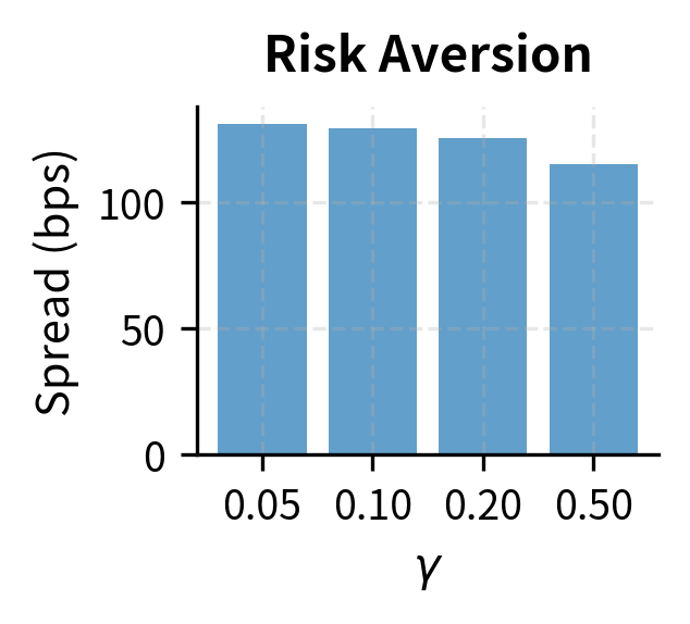
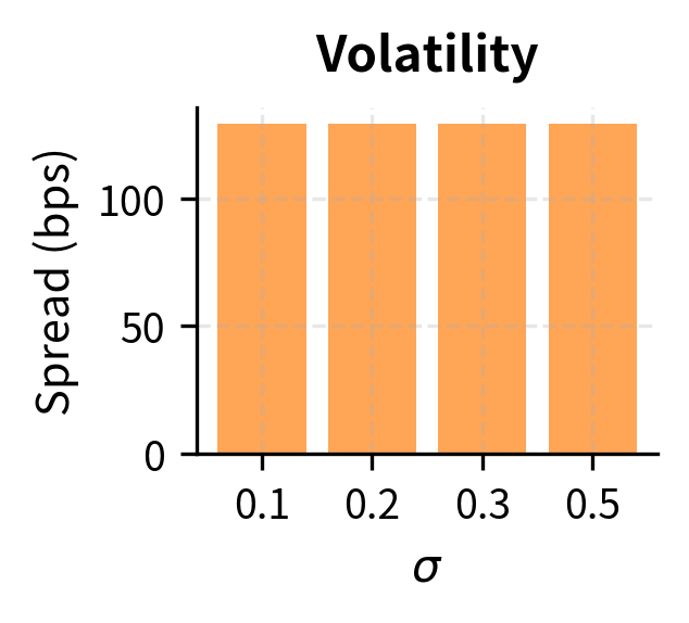
The sensitivity analysis reveals several important relationships that guide practical implementation:
- Higher risk aversion leads to wider spreads; more cautious traders demand greater compensation for bearing inventory risk. If you have limited capital or strict risk limits, you would appropriately use a higher gamma value.
- Higher volatility requires wider spreads to compensate for greater inventory risk. This explains why spreads widen during periods of market stress and narrow during calm periods. You dynamically adjust estimates based on recent realized volatility.
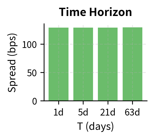
- Longer horizons allow wider spreads because there's more time for adverse price moves. This is counterintuitive at first: one might think that more time allows prices to revert. However, the model captures the fact that more time means more uncertainty, and you must be compensated for bearing this uncertainty.
Implementing a Market Making Simulation
Let's build a complete simulation to see how these concepts work together in practice. We'll simulate your strategy using the Avellaneda-Stoikov model over a trading day. This simulation will illustrate how the theoretical framework translates into actual trading behavior and outcomes.
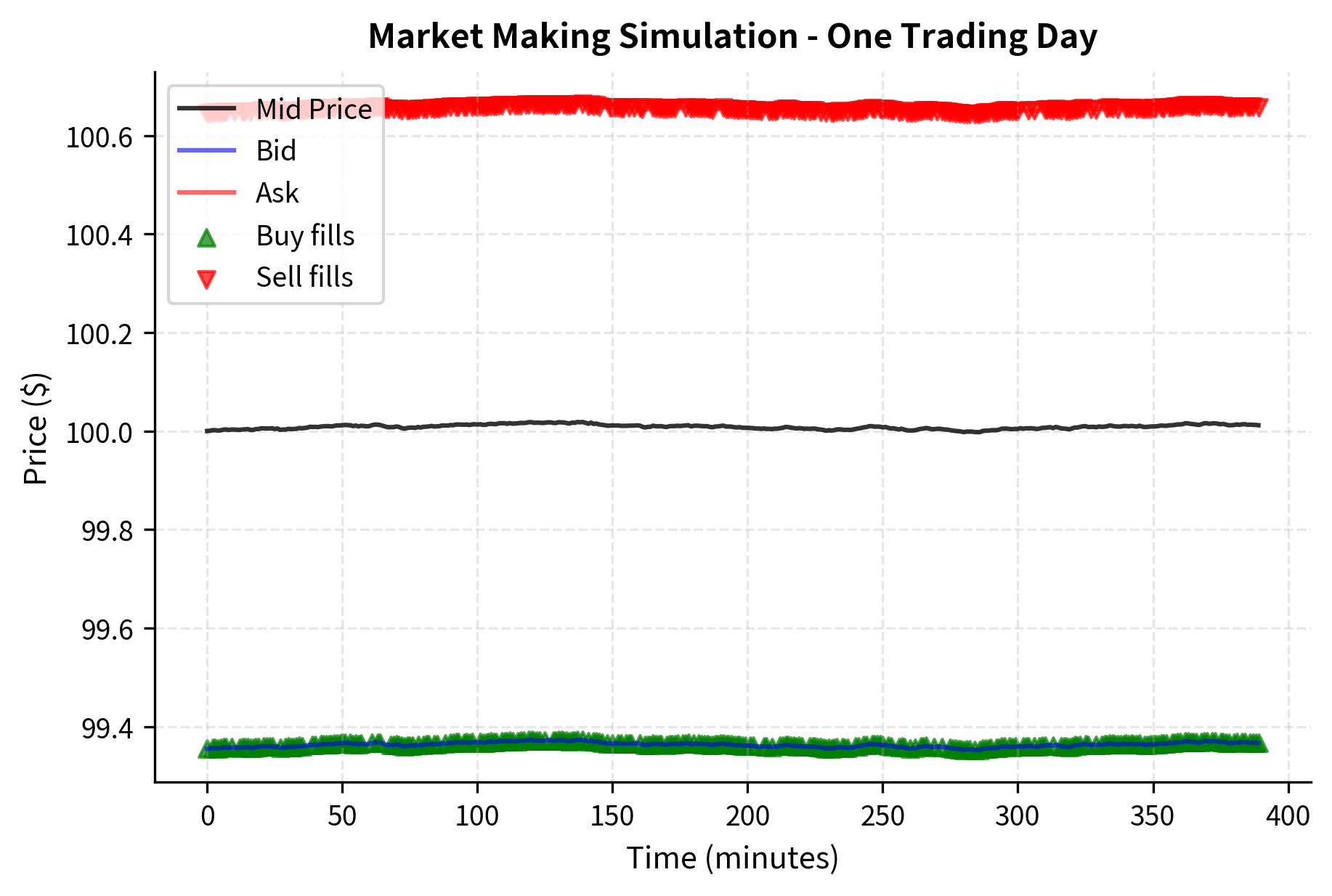
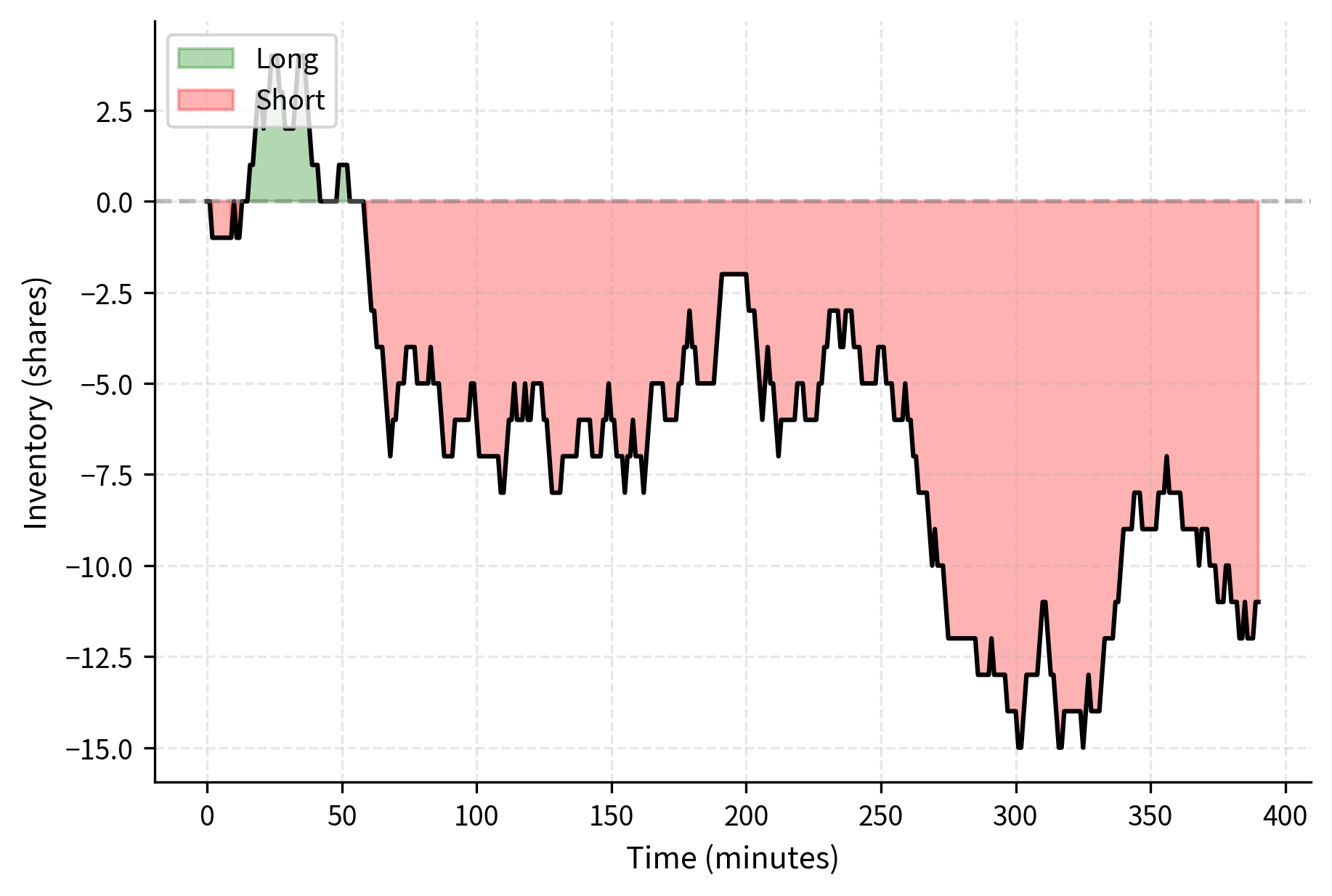
The simulation illustrates how the market making strategy works in practice. The top panel shows the mid price evolution with your bid and ask quotes, while trade executions are marked with triangles. The bottom panel shows how inventory evolves over time. Notice how it tends to fluctuate around zero because the quotes encourage mean reversion. When inventory drifts positive, the lower quotes attract sellers to buy from you, pulling inventory back down. When inventory drifts negative, the higher quotes attract buyers to sell to you.
Key Parameters
The key parameters for the market making simulation are:
- S0: Initial mid price. The starting point for the asset price simulation. This anchors all price calculations and determines the dollar value of positions.
- σ: Annualized volatility (sigma). Higher volatility increases inventory risk and widens spreads. This parameter must be estimated from recent market data and updated regularly.
- γ: Risk aversion parameter (gamma). Controls how aggressively you adjust quotes to manage inventory. Higher values lead to more aggressive inventory management but potentially less competitive quotes.
- k: Order book density. Determines how quickly the probability of a fill decays as quotes move away from the mid price. This parameter captures market-specific characteristics of order flow.
- A: Baseline arrival rate (lambda_base). The expected number of orders per unit time when quoting at the mid price. This sets the overall activity level of the simulation.
Risk Management for Market Makers
Successful market making requires sophisticated risk management beyond the theoretical models. Here we examine practical considerations that you must address in real-world implementation. The Avellaneda-Stoikov model provides a valuable framework, but you must augment it with additional safeguards and monitoring systems.
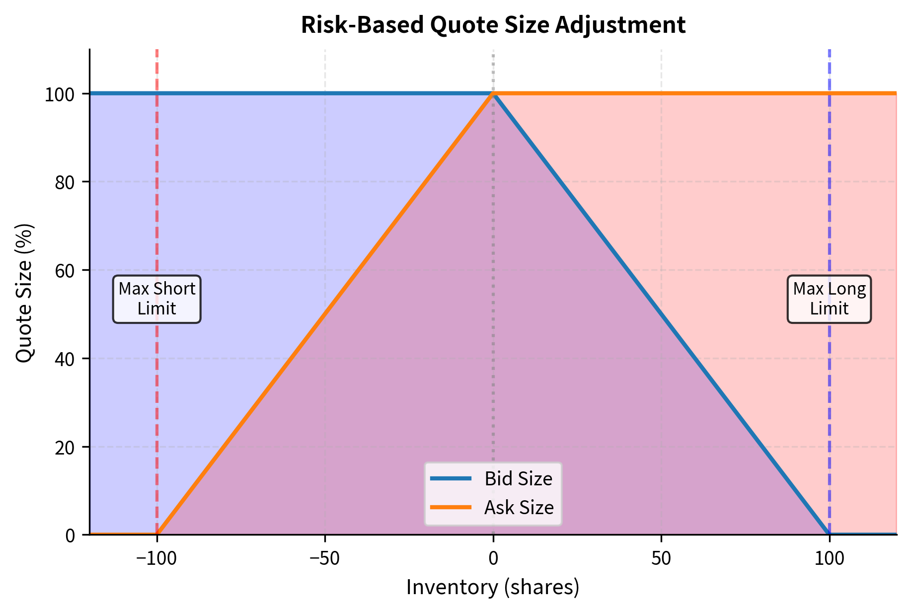
Position Limits and Circuit Breakers
You should typically impose hard limits on inventory positions. These limits serve as a safety mechanism to prevent catastrophic losses when models fail or market conditions become extreme. When inventory approaches these limits, you must take defensive action:
Volatility Regime Detection
You must adjust your behavior during high-volatility periods. Building on our discussion of volatility modeling in Part III, we can use realized volatility to dynamically adjust spreads. When volatility spikes, the Avellaneda-Stoikov model naturally suggests wider spreads, but the adjustment may need to be more aggressive than the model alone would suggest:
End-of-Day Risk
You face particular risk at the end of the trading day. Any remaining inventory must either be carried overnight (exposure to overnight gaps) or liquidated (potentially at unfavorable prices). The Avellaneda-Stoikov model captures this through the term; as time to horizon shrinks, the urgency to flatten inventory increases. This urgency manifests as more aggressive quote adjustment: you become increasingly willing to trade at unfavorable prices to avoid the even greater risk of holding overnight positions.
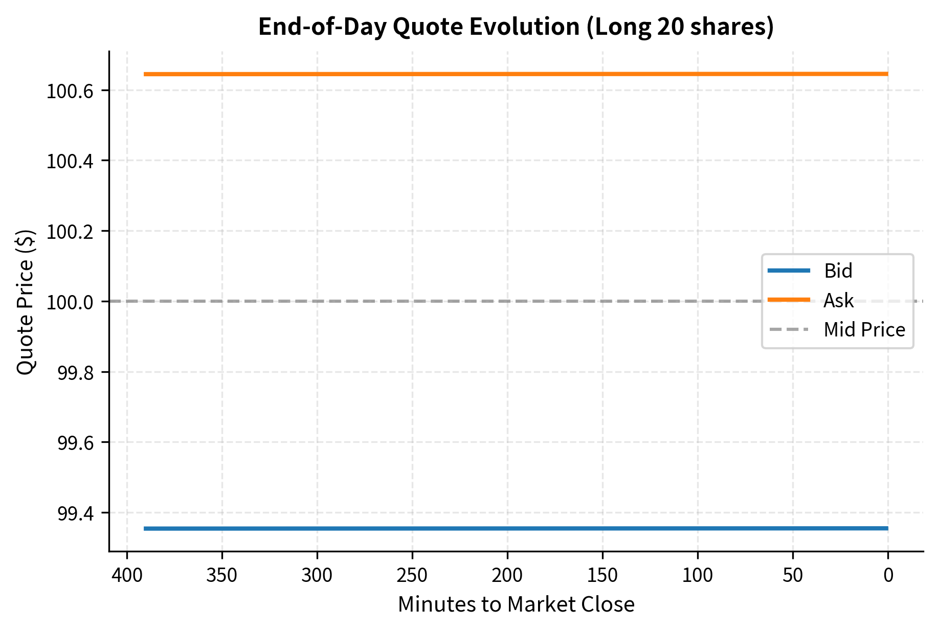
The figure shows how you, holding 20 shares long, would adjust quotes throughout the day. As the close approaches, both bid and ask drop dramatically; you are increasingly willing to sell at lower prices to avoid overnight risk. The speed of this adjustment accelerates as the close nears, reflecting the non-linear increase in urgency as time runs out.
The Role of Speed and Technology
Modern market making is as much about technology as about models. The concepts we've discussed in this chapter assume you can update quotes instantaneously, but in practice there's always latency, the time between deciding to change a quote and that change taking effect in the market. This latency creates vulnerability to adverse selection, as faster participants can trade against stale quotes.
The Speed Arms Race
When prices move, you must cancel or update your stale quotes. If you are slow to cancel a sell order when prices rise, you risk being "picked off," having your order executed at a now-unfavorable price. This creates intense competition on latency, where firms invest enormous resources to gain even microsecond advantages:
- Co-location: Placing servers in the same data center as the exchange minimizes the physical distance that signals must travel
- FPGA/ASIC: Custom hardware for sub-microsecond processing bypasses the overhead of general-purpose computing
- Microwave links: Faster-than-fiber communication between exchanges exploits the physics of electromagnetic wave propagation
- Optimized code: Every nanosecond matters, driving investment in highly optimized, often hardware-specific software
The upcoming chapter on High-Frequency Trading and Latency Arbitrage will explore these technological considerations in depth.
Quote Lifetime and Fill Rates
Your speed determines how long your quotes are "live" and vulnerable to adverse selection. We can estimate the expected adverse price movement during a latency period using the square-root-of-time rule for diffusion processes. This rule follows from the properties of Brownian motion: the standard deviation of price changes grows with the square root of time.
where:
- : expected price move magnitude
- : price volatility per millisecond
- : latency in milliseconds
Assuming a portion of these moves (e.g., 50%) result in you being "picked off" by faster traders, we can quantify the cost of latency.
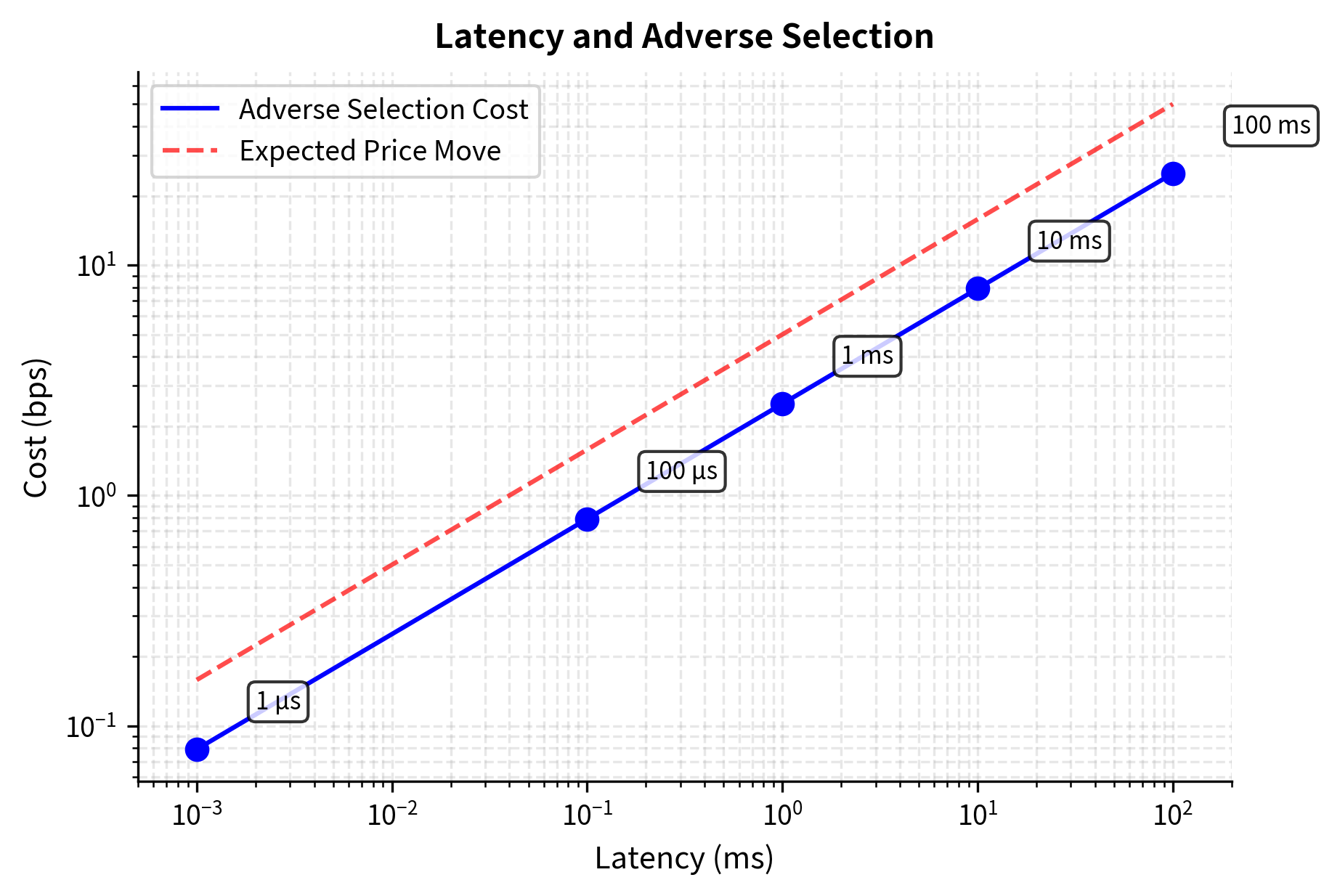
This simplified analysis shows why latency matters: if you are slower, you face higher adverse selection costs. A 100-millisecond delay might seem negligible to human perception, but in fast-moving markets, it can mean significant losses to faster traders who exploit stale quotes. The economics of latency explain why market making has become dominated by technology-intensive firms with the resources to compete at the frontier of speed.
Limitations and Impact
Quantitative market making models provide valuable frameworks for decision-making, but you must understand their constraints. This section examines both the theoretical limitations of the models and the practical challenges of real-world implementation.
Model Limitations
The quantitative models we've examined provide valuable intuition but have important limitations that you must understand:
The Avellaneda-Stoikov model assumes continuous trading, Gaussian price dynamics, and specific functional forms for order arrival rates. Real markets feature discrete ticks, fat-tailed distributions, and complex order flow dynamics. The model also treats all trades as uninformed, ignoring the adverse selection problem. This means the model's optimal quotes may be too aggressive in markets with significant informed trading.
Parameter estimation presents a significant challenge. The model requires values for (risk aversion) and (order book sensitivity), which are difficult to measure directly. You often calibrate these to historical data, but parameters may vary significantly across market conditions. A model calibrated to calm market conditions may perform poorly during periods of stress.
Market impact is largely ignored in basic models. Your own trading can move prices, especially in less liquid instruments. More sophisticated models incorporate this feedback effect, but doing so substantially increases complexity.
Real market making also involves multiple instruments traded simultaneously. Inventory in one stock may be partially hedged by positions in correlated stocks, ETFs, or futures. Multi-asset inventory management is considerably more complex than single-instrument models suggest, requiring portfolio-level optimization.
Practical Challenges
Beyond model limitations, real-world market making faces operational challenges that can be as important as theoretical considerations:
- Technology costs: Building and maintaining a competitive trading infrastructure requires substantial investment in hardware, software, and connectivity. These fixed costs create barriers to entry and economies of scale.
- Regulatory requirements: You might have affirmative obligations to provide liquidity and maintain orderly markets, particularly if you hold designated market maker status. These obligations can force you to provide liquidity even when it is unprofitable.
- Inventory financing: Carrying positions requires capital and creates balance sheet exposure. The cost of capital affects the profitability threshold for market making activities.
- Model risk: Systematic errors in models can lead to persistent losses before detection. Robust monitoring and model validation processes are essential.
Impact on Markets
Quantitative market making has fundamentally transformed financial markets over the past two decades. Bid-ask spreads have compressed dramatically, from eighths of a dollar to pennies or fractions of pennies. This benefits investors through lower transaction costs. A retail investor buying 100 shares of stock today pays a fraction of the transaction costs that would have applied in the 1990s.
However, the benefits come with trade-offs. Flash crashes, like the May 2010 event where the Dow Jones dropped nearly 1,000 points in minutes, revealed how quickly liquidity can evaporate when automated market makers simultaneously pull quotes. The reliance on speed has created barriers to entry, concentrating liquidity provision among a handful of highly capitalized technology firms.
The ongoing evolution of market structure, including changes to maker-taker fee models, minimum tick sizes, and transparency requirements, continues to reshape the competitive landscape for you. Understanding these dynamics is essential for anyone involved in quantitative trading or market design.
Summary
This chapter explored the economics, models, and risks of quantitative market making:
Core economics: You earn the bid-ask spread by providing immediacy to other traders. You buy at the bid and sell at the ask, capturing the difference. Profitability depends on managing inventory risk and avoiding adverse selection.
Inventory risk: Accumulated positions expose you to directional price risk. The Avellaneda-Stoikov model provides optimal quotes that shift based on inventory, encouraging mean reversion. When long, quotes shift lower; when short, quotes shift higher.
Adverse selection: Informed traders profit at your expense by trading when they have superior information. Spreads must be wide enough to compensate for losses to informed flow while remaining competitive for uninformed flow.
The Avellaneda-Stoikov model: This foundational framework produces optimal bid and ask quotes based on current inventory, volatility, risk aversion, and time horizon. The model introduces the reservation price concept: your private valuation adjusted for inventory risk.
Risk management: Practical market making requires position limits, volatility regime detection, and end-of-day protocols. The model parameters require careful calibration and ongoing monitoring.
Technology and speed: Modern market making is a technology race. Latency determines adverse selection exposure; if you are slower, you face higher costs from stale quotes being picked off. The upcoming chapter on High-Frequency Trading will explore these technological dimensions further.
Market making sits at the intersection of financial theory and engineering practice. The models provide a theoretical foundation, but successful implementation requires mastering the operational and technological challenges that define modern electronic markets.
Quiz
Ready to test your understanding? Take this quick quiz to reinforce what you've learned about market making and liquidity provision.

Comments