High-Frequency Trading: Latency Arbitrage & Market Making

In the previous chapter, we explored market making and liquidity provision, where traders profit by capturing bid-ask spreads while managing inventory risk. High-frequency trading (HFT) takes these concepts to their logical extreme: holding periods are measured in milliseconds. Trading infrastructure is optimized for microsecond response times. Profit margins are so thin that success depends on executing millions of trades with near-perfect consistency.

High-frequency trading emerged in the early 2000s as electronic markets replaced human floor traders. What began as simple automation of existing strategies evolved into a sophisticated ecosystem where algorithms compete with each microsecond of latency advantage worth millions of dollars. Firms invest in microwave towers and hollow-core fiber optics to shave microseconds off transmission times between exchanges. This infrastructure investment reflects the extraordinary value of marginal speed advantages. By some estimates, HFT accounts for 50 to 60% of U.S. equity trading volume and fundamentally reshapes market microstructure.

The defining characteristic of HFT is not the strategies themselves. Many are conceptually similar to traditional arbitrage and market making. Instead, it's the timescales involved that define HFT. A statistical arbitrage fund might hold positions for days or weeks, while an HFT firm might hold for seconds or less. With traditional strategies, you might execute dozens of trades per day. An HFT algorithm executes thousands per second. This compression of time creates both opportunities and challenges that distinguish HFT from other quantitative strategies.

This chapter examines the core strategies employed by HFT firms, the technology infrastructure that makes sub-millisecond trading possible, and the economic and regulatory forces shaping this industry. You'll see how concepts from earlier chapters (no-arbitrage pricing from Part III, market making from the previous chapter, and statistical analysis from Part I) combine with cutting-edge technology to create one of the most competitive domains in finance.

Before diving into specific strategies, we need to understand the fundamental economics that make HFT viable. The key insight is that HFT profits come from exploiting tiny, fleeting inefficiencies at enormous scale.

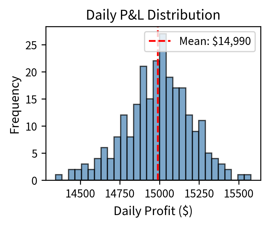
Consider a simple example. An HFT firm identifies a price discrepancy of $0.01 between two exchanges. After transaction costs of $0.005 per share (round trip), the profit is $0.005 per share. This seems negligible, but if you can execute this trade 10,000 times per day across 500 different securities, daily profits reach $25,000. Over a year of 252 trading days, this accumulates to over $6 million, from a strategy that earns half a penny per trade.

The economics of HFT are characterized by several key features:

• High Sharpe ratios: HFT strategies make many small, consistent profits, so their risk-adjusted returns are often extremely high.

The Sharpe ratio quantifies risk-adjusted returns by measuring how much excess return is earned per unit of risk. It provides a standardized metric for comparing strategies with different risk profiles, making it particularly valuable for evaluating HFT strategies.

The Sharpe ratio is calculated as:

where:

• $E[R_p]$: expected portfolio return (annualized percentage)
• $R_f$: risk-free rate (annualized percentage, typically 3-month Treasury bill rate)
• $\sigma_p$: portfolio return standard deviation (annualized percentage, measuring volatility)

To understand why this formula captures risk-adjusted performance, consider what each component contributes. The numerator $E[R_p] - R_f$ represents the excess return: the compensation investors receive for taking risk beyond the risk-free rate. This excess return is what truly matters for evaluating a strategy, because any investor can earn $R_f$ simply by purchasing Treasury bills. The key question is whether the strategy's additional risk-taking is rewarded with commensurate returns.

The denominator $\sigma_p$ normalizes this excess return by the volatility incurred to achieve it. Volatility measures the dispersion of returns around the mean, capturing the uncertainty an investor experiences while holding the strategy. A strategy that earns 10% excess return with 5% volatility is providing two units of return per unit of risk, while a strategy earning the same 10% with 20% volatility provides only half a unit of return per unit of risk.

By dividing excess return by volatility, we obtain a ratio that answers a fundamental question: "How much return do I get per unit of risk?" This normalization allows fair comparison between strategies with different risk profiles.

A conservative strategy with low volatility and modest returns can be meaningfully compared to an aggressive strategy with high volatility and high returns, because both are evaluated on the same risk-adjusted basis.

Higher Sharpe ratios indicate better risk-adjusted performance. A Sharpe ratio of 1.0 means the strategy earns one unit of excess return for each unit of volatility taken. A ratio of 2.0 means it earns two units of excess return per unit of volatility. Traditional interpretations suggest that a Sharpe ratio above 1.0 is good, above 2.0 is very good, and above 3.0 is excellent.

HFT strategies often achieve Sharpe ratios of 10 or higher because making many small, consistent profits reduces volatility relative to expected returns. This remarkable risk-adjusted performance emerges from a statistical phenomenon: the law of large numbers transforms highly variable individual trades into remarkably consistent aggregate returns. When thousands of trades are executed daily, each with a small positive expected value, the randomness of individual outcomes averages out, producing steady daily profits with low day-to-day variation. For comparison, traditional hedge funds typically achieve Sharpe ratios of 1 to 2, making HFT's risk-adjusted returns exceptional by any standard measure.

• Capacity constraints: The opportunities exploited by HFT are finite. As more capital chases these strategies, profits per trade decline. This creates natural limits on how much capital HFT strategies can deploy profitably.

• High fixed costs: The infrastructure required for competitive HFT, including co-location, direct data feeds, and specialized hardware, requires millions of dollars in upfront investment and ongoing maintenance.

• Winner-take-most dynamics: In many HFT strategies, being slightly faster than competitors captures most of the available profit. This creates an arms race where firms continuously invest in speed improvements.

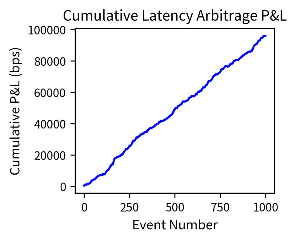
The simulation illustrates a key HFT characteristic: despite the tiny expected profit per trade, the law of large numbers transforms highly variable individual trades into remarkably consistent daily returns. The annualized Sharpe ratio represents exceptional risk-adjusted performance because making many trades per day reduces daily volatility relative to expected daily profit. For comparison, traditional hedge funds typically achieve Sharpe ratios of 1 to 2, making HFT's risk-adjusted returns exceptional.

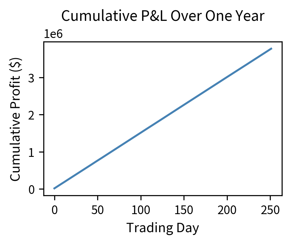
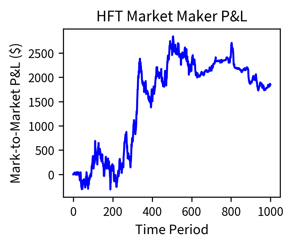
The cumulative P&L chart shows the characteristic "staircase" pattern of successful HFT strategies: steady, consistent gains with minimal drawdowns. This consistency is what allows HFT firms to operate with high leverage and explains their appeal to investors.

The key parameters for HFT strategy simulation are:

• trades_per_day: Number of trades executed daily, with higher values improving statistical consistency through the law of large numbers, as more independent outcomes average together to produce stable daily results.
• profit_per_trade_mean: Expected profit per share per trade. Even tiny values (e.g., $0.003) accumulate significantly at scale when multiplied across thousands of daily trades.
• profit_per_trade_std: Volatility of individual trade profits, with high variance at the trade level becoming low variance at the daily level through aggregation effects.
• shares_per_trade: Position size per trade. Larger sizes amplify both profits and risks proportionally.
• trading_days: Number of trading days per year (typically 252), used to annualize metrics like Sharpe ratio by accounting for the compounding effect across all trading sessions.

Cross-market arbitrage is perhaps the most intuitive HFT strategy: buy an asset where it's cheap and simultaneously sell it where it's expensive. While the concept is simple, the implementation requires sophisticated technology to identify and capture fleeting price discrepancies.

Cross-market arbitrage opportunities arise in several contexts:

• Exchange arbitrage: Exploits price differences for the same security listed on multiple exchanges. A stock like Apple trades on NYSE, NASDAQ, and various electronic communication networks (ECNs). Price discrepancies arise due to latency in information propagation, differences in order flow, and temporary imbalances in supply and demand.

• ETF arbitrage: Exploits discrepancies between an ETF's market price and its net asset value (NAV). ETFs should trade at prices very close to the value of their underlying holdings. When discrepancies arise, arbitrageurs buy the cheaper instrument and sell the more expensive one.

• Futures-spot arbitrage: Exploits deviations from the theoretical relationship between futures and spot prices. The cost-of-carry model establishes the no-arbitrage relationship between futures and spot prices through a compelling economic argument. Consider an investor deciding between two strategies: (1) buying a futures contract for delivery at time $T$, or (2) buying the underlying asset now and holding it until $T$. These strategies must have equal cost; otherwise, arbitrage opportunities exist.

To understand why equal cost is necessary, consider what would happen if the strategies had different costs. If buying spot were cheaper, every investor would prefer that route, driving up the spot price. If the futures route were cheaper, investors would flock to futures, driving up the futures price. This competitive pressure ensures that in equilibrium, both paths to owning the asset at time $T$ must cost the same.

When holding the spot asset, the investor incurs financing costs at rate $r$ but receives dividend income at rate $q$. The net cost of carry is $(r-q)$: the difference between financing costs paid and dividend income received. This net cost grows over time, and under continuous compounding, the growth is exponential with time $T$. To see why, consider the growth factor for the carrying cost:

This exponential term captures how the net cost $(r-q)$ compounds continuously over time period $T$. The mathematical function $e^x$ (the exponential function) is the natural way to express continuous compounding, where interest is reinvested infinitely often within each time period. The futures price must therefore equal the spot price adjusted for this carrying cost:

where:

• $F_0$: futures price at time 0 (dollars per unit)
• $S_0$: spot price at time 0 (dollars per unit)
• $r$: risk-free interest rate (annualized, continuous compounding, e.g., 0.05 for 5%)
• $q$: dividend yield (annualized, continuous compounding, e.g., 0.02 for 2%)
• $T$: time to expiration (years, e.g., 0.25 for 3 months)
• $e^{(r-q)T}$: continuous compounding factor that grows the spot price forward to account for carrying costs

The exponent $(r-q)$ captures the net carrying cost and reveals an important economic insight. This term determines whether futures trade at a premium or discount to spot:

• When $r > q$: financing costs exceed dividend income, so futures trade at a premium to spot (contango). In this situation, holding the spot asset is expensive relative to the income it generates, so investors require compensation in the form of higher futures prices.
• When $r < q$: dividend income exceeds financing costs, so futures trade at a discount (backwardation). Here, holding the spot asset is attractive because it generates more income than it costs to finance, so investors accept lower futures prices.
• When $r = q$: the futures price equals the spot price (no net carry). The benefits and costs of holding the asset exactly offset.

Why does this formula prevent arbitrage? Suppose $F_0 > S_0 e^{(r-q)T}$, meaning futures are overpriced relative to the theoretical value. You could execute the following strategy:

1. Short the futures contract at $F_0$ (agree to deliver the asset at expiration for price $F_0$)
2. Borrow $S_0$ at rate $r$ to buy the spot asset now
3. Hold the asset until expiration, collecting dividends at rate $q$
4. Deliver the asset at expiration for price $F_0$

The profit from this arbitrage would be:

where:

• $F_0$: proceeds from delivering the asset via the futures contract
• $S_0 e^{(r-q)T}$: total cost of the position after accounting for financing costs (growing at rate $r$) and dividend income (reducing costs at rate $q$)

Since this profit is risk-free and requires no capital, arbitrageurs would execute this trade until the price discrepancy disappears. Similarly, if $F_0 < S_0 e^{(r-q)T}$, the reverse arbitrage (buy futures, short spot) would be profitable. Therefore, in equilibrium, $F_0 = S_0 e^{(r-q)T}$ must hold.

• Cross-listed securities arbitrage: Exploits price differences for securities listed in multiple countries. A company might have shares trading in New York and London, with prices that should be equivalent after adjusting for exchange rates.

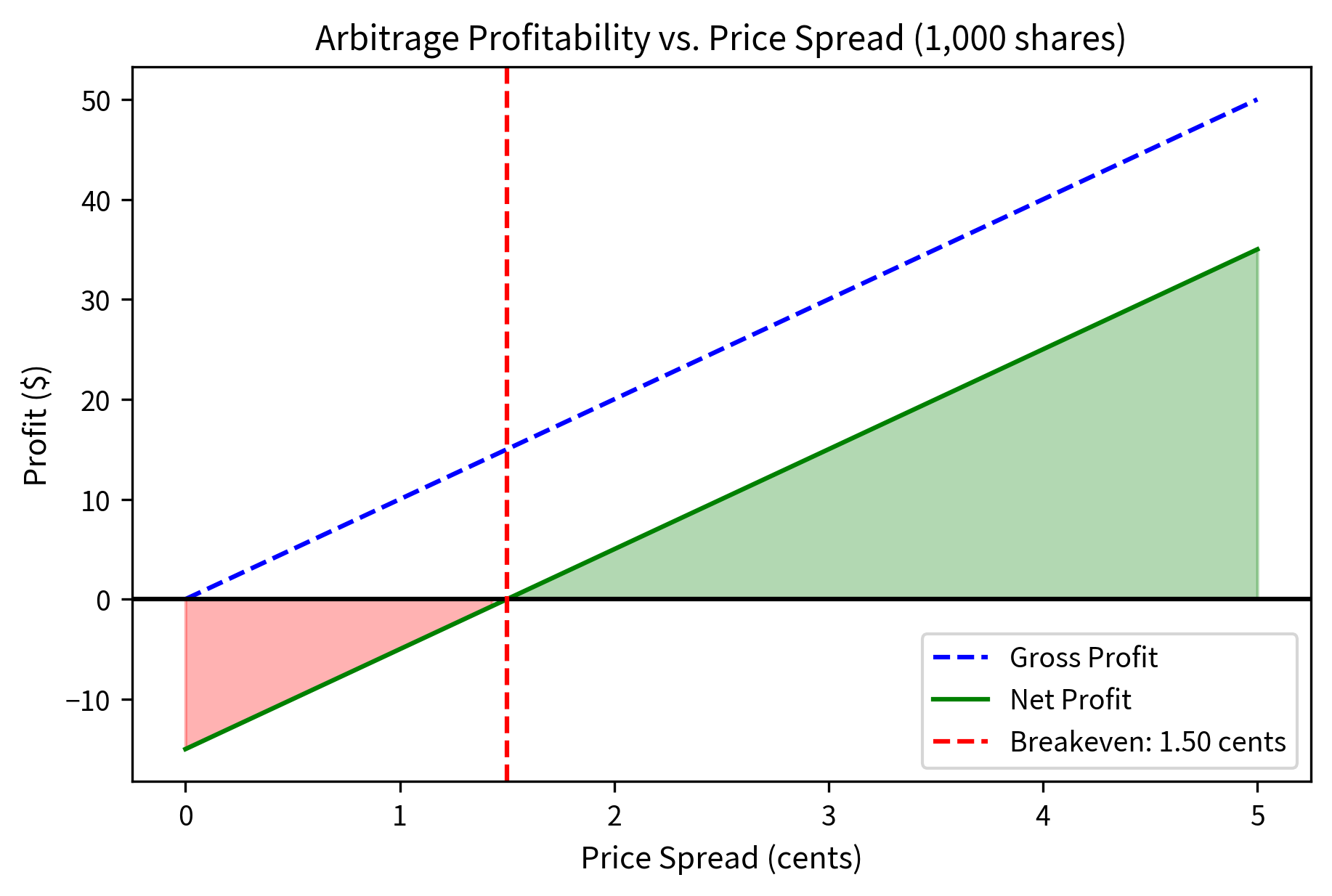
Let's examine the mechanics of exchange arbitrage in detail. Suppose Apple stock is trading at $150.00 on NYSE and $150.02 on NASDAQ. You could:

1. Buy 1,000 shares on NYSE at $150.00 (cost: $150,000)
2. Simultaneously sell 1,000 shares on NASDAQ at $150.02 (proceeds: $150,020)
3. Net profit before costs: $20

However, several factors complicate this simple picture.

The analysis demonstrates why speed is critical in cross-market arbitrage. The gross profit on 1,000 shares is reduced by transaction costs and slippage, leaving a small net profit per share. The profitable window exists only while the price discrepancy exceeds the breakeven spread: faster traders see and act on opportunities before prices converge, while slower traders arrive to find the arbitrage has already been captured.

The key parameters for cross-market arbitrage are:

• price_a: Lower price on the buy side exchange (dollars per share), which determines the cost basis for the arbitrage position.
• price_b: Higher price on the sell side exchange (dollars per share), which determines the revenue when closing the position.
• shares: Number of shares to trade, with larger positions amplifying both profits and costs proportionally.
• fee_per_share: Exchange fee for removing liquidity (dollars per share). These transaction costs erode gross profits and represent a fixed hurdle that must be overcome.
• slippage_bps: Expected price movement against the trader during execution (basis points), representing adverse selection and execution timing risk that grows with position size and market volatility.
• breakeven_spread: Minimum price difference required for profitability after costs (dollars per share), a critical threshold determining whether arbitrage is viable and representing the entry barrier for slower competitors.

ETF arbitrage is more complex because it involves trading a basket of securities against the ETF itself. The key participants are authorized participants (APs), typically large financial institutions, who can create or redeem ETF shares directly with the fund.

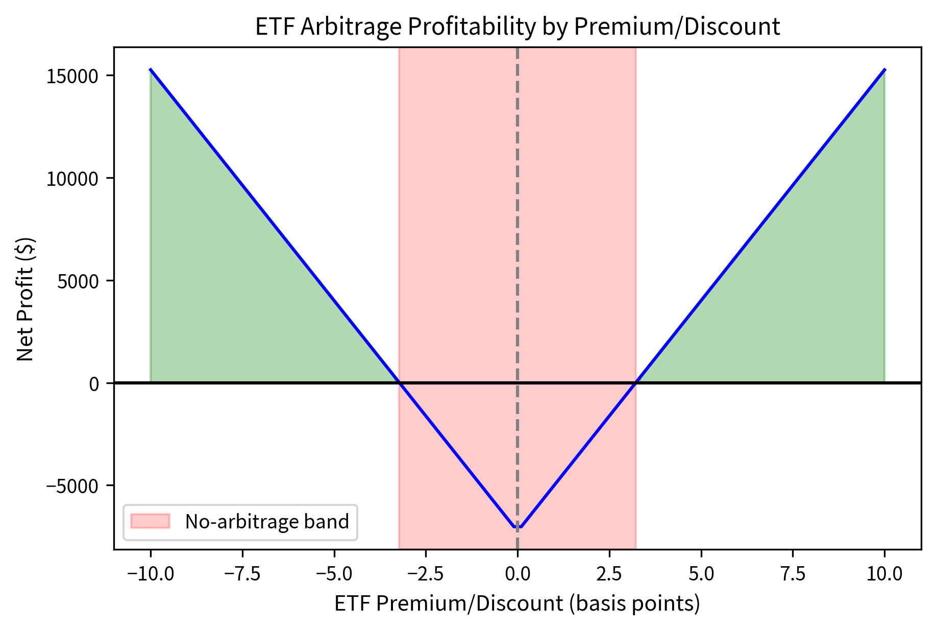
When an ETF trades at a premium to NAV, you can execute the following strategy:

1. Buy the underlying basket of securities
2. Deliver the basket to the ETF issuer to create new ETF shares
3. Sell the newly created ETF shares at the premium price
4. Profit equals the premium minus transaction costs and creation fees

When an ETF trades at a discount to NAV, the process reverses.

The analysis shows that the premium generates substantial profits at scale. For one creation unit (50,000 shares), the gross profit exceeds total costs, yielding a net profit. However, the breakeven premium demonstrates why only well-capitalized, low-cost traders can profitably engage in ETF arbitrage. The margin between the actual premium and breakeven is narrow, requiring precise execution and minimal slippage.

The key parameters for ETF arbitrage are:

• etf_price: Current ETF market price (dollars per share), compared to NAV to identify premium or discount conditions.
• nav: Net asset value per ETF share (dollars per share), representing the theoretical fair value based on underlying holdings and serving as the benchmark for arbitrage calculations.
• shares_per_creation_unit: Number of shares in one creation/redemption unit (typically 50,000), the minimum size for direct creation/redemption with the fund issuer.
• creation_fee: Fixed fee charged by the ETF issuer for creation or redemption (dollars), representing administrative costs that must be overcome regardless of position size.
• basket_execution_cost_bps: Cost to trade the underlying basket of securities (basis points), including commissions and market impact from trading potentially hundreds of individual stocks.
• etf_execution_cost_bps: Cost to trade the ETF itself (basis points), typically lower than basket costs due to better liquidity concentration in a single instrument.

Latency arbitrage exploits the fact that information takes time to propagate across markets. At the speed of light through fiber optic cable, a price change in Chicago takes approximately 7-8 milliseconds to reach New York, while microwave transmission can reduce this to about 4 milliseconds. During this window, a trader with faster access to the price change can act before competitors.

Consider the following scenario: the S&P 500 E-mini futures contract trades in Chicago, while SPY (the S&P 500 ETF) trades in New York. When new information arrives in Chicago and moves the futures price, it takes time for that information to reach New York and affect SPY's price.

Positioned in both locations, you can execute the following strategy:

1. Observe a futures price movement in Chicago
2. Immediately transmit the information to New York via the fastest available channel
3. Trade SPY in New York before the broader market incorporates the information
4. Profit from the predictable price adjustment

Latency arbitrage depends on predicting how a target instrument, like SPY in New York, will adjust when a signal instrument, such as S&P 500 futures in Chicago, moves. The key insight is that highly correlated instruments must eventually move together, but information propagation takes time. During this latency window, you can act on the predictable price adjustment.

The prediction model uses a simple linear relationship that emerges from the economic connection between related instruments. When the signal instrument moves by amount $\Delta P_{\text{signal}}$, we predict the target instrument will move by:

where:

• $\Delta P_{\text{target}}$: expected price change in the target instrument (dollars, e.g., SPY in New York)
• $\Delta P_{\text{signal}}$: observed price change in the signal instrument (dollars, e.g., S&P 500 futures in Chicago)
• $\beta$: sensitivity coefficient (dimensionless ratio, typically 0.95 to 1.0 for an ETF and its underlying index)

The parameter $\beta$ quantifies the statistical relationship between the instruments, serving as the bridge between observing the signal and predicting the target's response. It answers a specific question: "When the signal moves $1, by how much does the target typically move?" This simple question captures the essence of the predictive model.

Estimating beta: This coefficient is estimated through regression analysis on historical paired price movements. By examining thousands of past instances where the signal instrument moved, we observe how the target instrument responded and extract the average sensitivity. The regression identifies the slope of the best-fit line relating signal changes to target changes, providing a data-driven estimate of $\beta$.

Why beta ≈ 1 for SPY: For an ETF like SPY that tracks the S&P 500 index, we expect beta approximately 1 because the relationship is built into the fund's structure:

• SPY's net asset value (NAV) directly depends on the S&P 500 index value by construction
• If S&P 500 futures jump $1, SPY's fair value also increases approximately$1 through this mechanical linkage
• No-arbitrage pricing forces SPY to track these movements closely, as deviations would create ETF arbitrage opportunities

However, $\beta$ might deviate slightly from 1.0 due to several practical factors:

• Tracking error (SPY's holdings may not perfectly match the index due to sampling or optimization)
• Transaction costs in the creation/redemption process create a band around fair value
• Market conditions (volatility can temporarily affect the relationship as liquidity providers adjust their behavior)

The arbitrage opportunity: During the latency window when futures have moved but SPY hasn't yet adjusted, you can:

1. Observe the futures move in Chicago
2. Predict SPY will move $\beta \Delta P_{\text{signal}}$
3. Trade in New York before other participants see the signal
4. Capture the predictable price adjustment as SPY converges to its new fair value

Profitability requirements: For this strategy to generate positive expected returns, several conditions must hold:

1. Accurate $\beta$ estimation (incorrect predictions lead to losses when the actual relationship differs from the model)
2. Sufficient speed advantage (the latency window must be long enough to execute before prices converge)
3. Low transaction costs (costs must be smaller than captured movements, requiring efficient execution infrastructure)

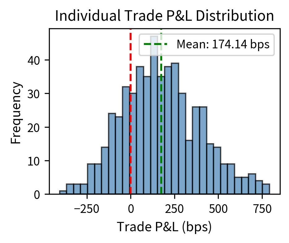
The simulation demonstrates the economics of latency arbitrage. The strategy executed many trades from the signal events observed: the total net P&L translates to tiny average profits per trade with a high win rate. The strategy captures a fraction of each expected price move due to its speed advantage. These tiny per-trade profits accumulate through high-frequency execution.

The key parameters for latency arbitrage simulation are:

• n_events: Number of signal events observed (e.g., 1000), with more events providing better statistical sampling of strategy performance.
• signal_volatility: Typical magnitude of signal price changes (basis points), representing market volatility that creates arbitrage opportunities.
• beta: Statistical sensitivity between signal and target instruments (dimensionless), quantifying how much the target moves when the signal moves and forming the core of the prediction model.
• latency_advantage_ms: Speed advantage over competitors (milliseconds), determining the time window for capturing moves before prices converge.
• market_response_time_ms: Time for market to fully adjust to signals (milliseconds), defining how long arbitrage opportunities persist before information is fully incorporated.
• execution_prob: Probability of successfully executing each trade (0 to 1), accounting for infrastructure reliability and competition for available liquidity.
• transaction_cost_bps: Round-trip transaction cost (basis points), determining minimum profitable signal threshold and representing the hurdle that must be cleared for profitable trading.

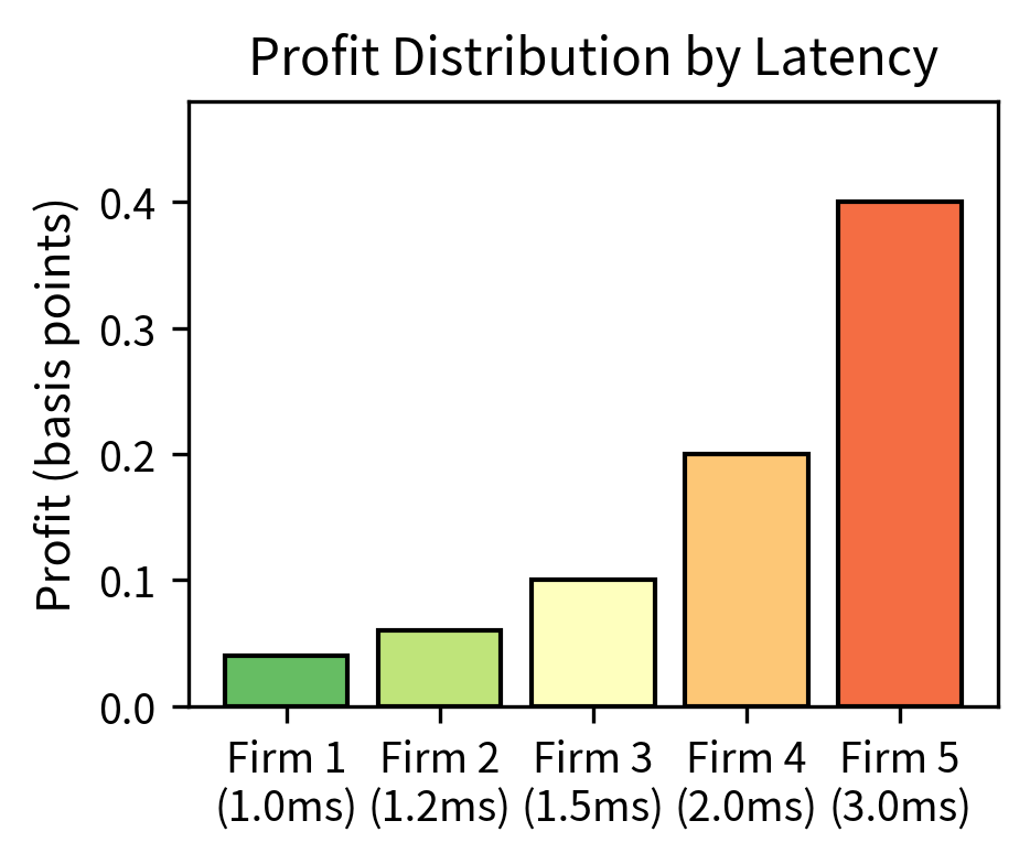
The profitability of latency arbitrage depends critically on relative speed. Being the fastest trader captures most of the available profit; being second-fastest may capture nothing. This creates intense competition to reduce latency.

The analysis demonstrates the "winner-take-most" nature of latency competition. The fastest firm captures the majority of the opportunity, while the second-fastest firm captures only a small fraction. Firms 3-5 capture even smaller fractions. This distribution shows that being the fastest matters more than being fast, explaining why HFT firms invest heavily in marginal speed improvements.

The key parameters for speed competition analysis are:

• latencies_ms: List of competitor latencies (milliseconds), determining relative speed advantages and establishing the competitive hierarchy.
• total_opportunity_bps: Total arbitrage opportunity per event (basis points), representing the value to be captured and divided among competitors.
• market_adjustment_ms: Time for market to fully adjust prices (milliseconds), defining the total window of opportunity during which profits can be captured.
• profit_shares: Fraction of opportunity captured by each competitor (0 to 1), showing winner-take-most dynamics where small speed differences translate to large profit differences.

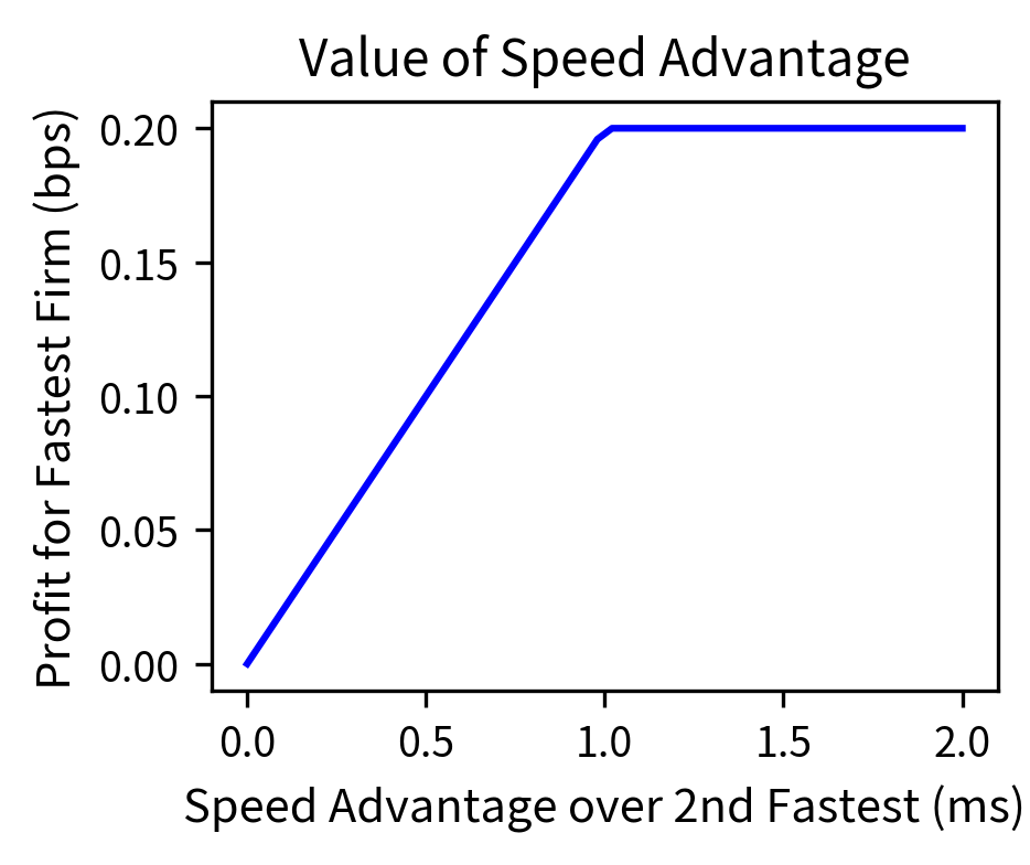
The right panel shows how the fastest firm's profit increases with their speed advantage. The relationship is roughly linear: each additional millisecond of speed advantage translates to approximately 0.2 basis points of additional profit per event. This quantifies the economic value of speed improvements and helps firms decide how much to invest in infrastructure.

The competitive dynamics of HFT have driven extraordinary investments in technology infrastructure. Understanding these systems helps explain why certain strategies are viable and how the industry has evolved.

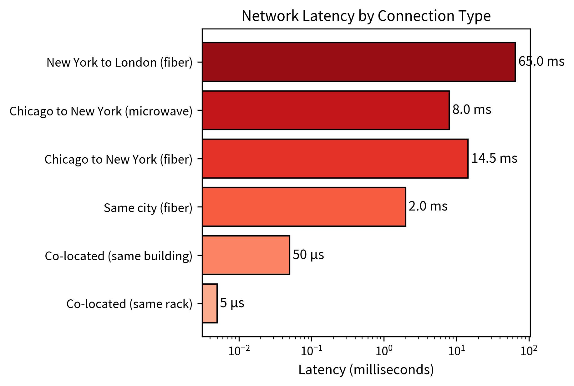
The most direct way to reduce latency is physical proximity to the exchange matching engine. Co-location services allow you to place your servers in the same data center as the exchange, minimizing the distance signals must travel.

The impact of co-location is substantial. Within a co-located facility, round-trip latency to the exchange might be 10 to 50 microseconds. From a remote data center in the same city, latency increases to 1 to 5 milliseconds. From across the country, latency might be 30 to 70 milliseconds.

Exchange data is distributed through two primary channels:

Consolidated feeds (like the Securities Information Processor or SIP) aggregate data from all exchanges into a single stream. These feeds are regulated to provide equal access but introduce latency due to aggregation and distribution overhead.

Direct feeds are proprietary data streams from individual exchanges. They deliver data faster than consolidated feeds and often contain additional information (such as full order book depth) not available in consolidated feeds.

The latency difference between direct and consolidated feeds can be several hundred microseconds, a significant disadvantage in HFT. This differential creates opportunities for you with direct feeds to react to price changes before they appear in consolidated data.

Beyond network infrastructure, HFT firms optimize every component of their trading systems.

Key hardware optimizations include:

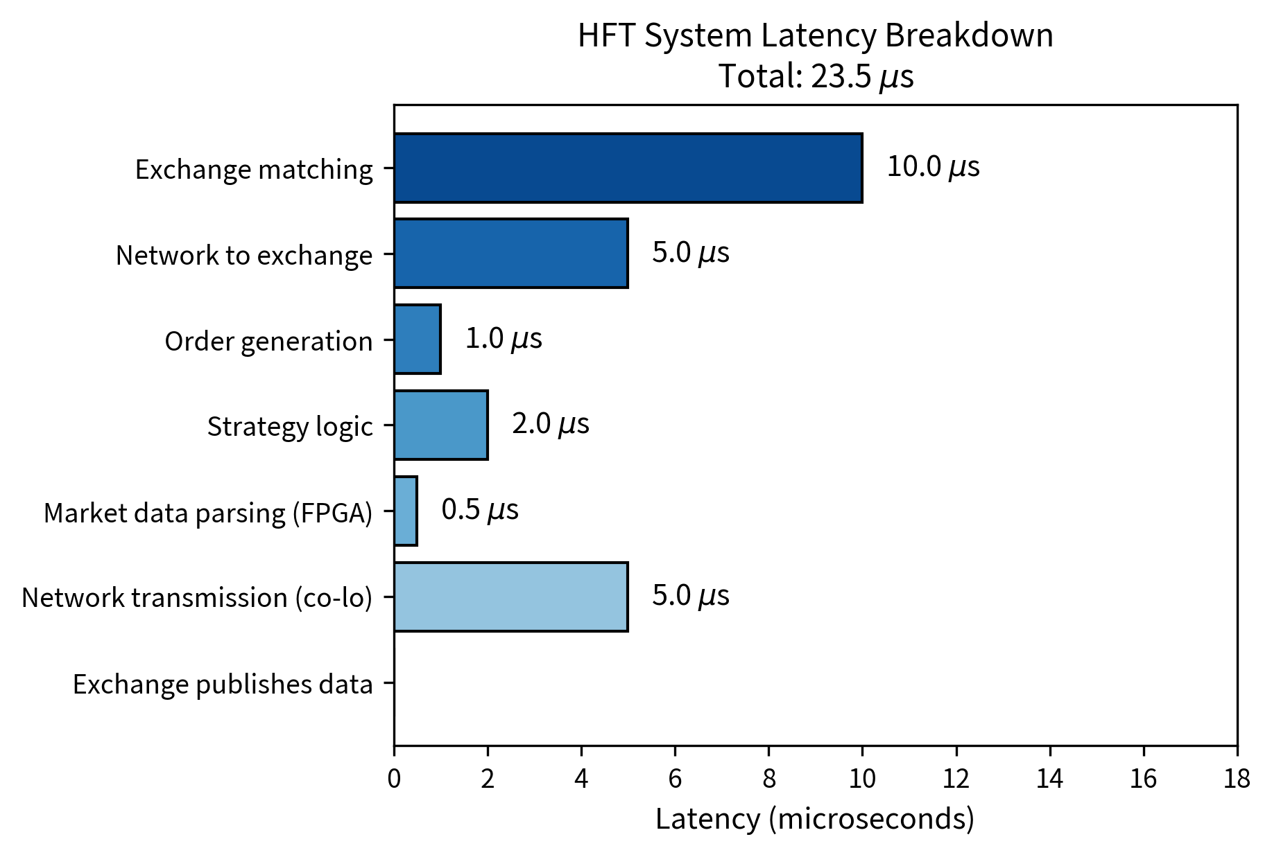
• Field Programmable Gate Arrays (FPGAs): Specialized chips that execute specific algorithms faster than general-purpose CPUs. An FPGA-based trading system can parse market data and generate orders in under 1 microsecond, compared to 10 to 100 microseconds for software-based systems

• Kernel bypass networking: Allows trading applications to send and receive network packets without involving the operating system kernel, reducing latency by tens of microseconds.

• Custom network cards: Hardware timestamping enables precise latency measurement and synchronization across distributed systems.

• Memory optimization: Ensures that frequently accessed data remains in CPU cache rather than main memory, reducing access time from nanoseconds to sub-nanosecond levels.

Many HFT firms operate as electronic market makers, building on the principles we covered in the previous chapter but implementing them at much higher speeds and with more sophisticated risk management.

High-frequency market makers continuously update their quotes to reflect changing market conditions. A key challenge is managing the risk of being "picked off," which occurs when your stale quotes are executed against by faster traders who have already seen a price change.

The quote update process involves these steps:

1. Receiving market data (prices, order flow, news)
2. Updating fair value estimate
3. Calculating new bid and ask quotes
4. Sending cancel messages for old quotes
5. Sending new quote messages

The entire cycle must complete faster than competitors can trade against your stale quotes.

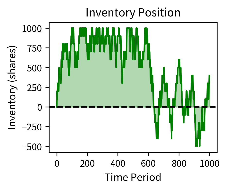
The simulation demonstrates successful HFT market making. The strategy generated profits with a strong Sharpe ratio, indicating excellent risk-adjusted returns, while the maximum drawdown occurred during periods of adverse price movement. The average absolute inventory stayed well below the 1,000 share limit, showing effective inventory management through position skewing. The consistent profits come from capturing bid-ask spreads while managing adverse selection risk.

The key parameters for HFT market maker simulation are:

• n_periods: Number of time periods simulated, with more periods better capturing long-term performance and ensuring statistical robustness.
• true_price_vol: True price volatility per period (percentage), representing market uncertainty that creates both risk and opportunity for market makers.
• spread_bps: Bid-ask spread quoted by market maker (basis points), determining gross profit per round-trip trade and representing compensation for providing liquidity.
• inventory_limit: Maximum inventory position (shares), a risk control preventing excessive exposure to directional price movements.
• fill_probability: Probability of quote being filled each period (0 to 1), representing trading frequency and interaction with order flow.
• adverse_selection_bps: Loss per fill due to informed traders (basis points), representing the cost of providing liquidity to better-informed counterparties who trade when prices are about to move.

As a sophisticated market maker, you analyze incoming order flow to detect patterns that predict future price movements. This involves:

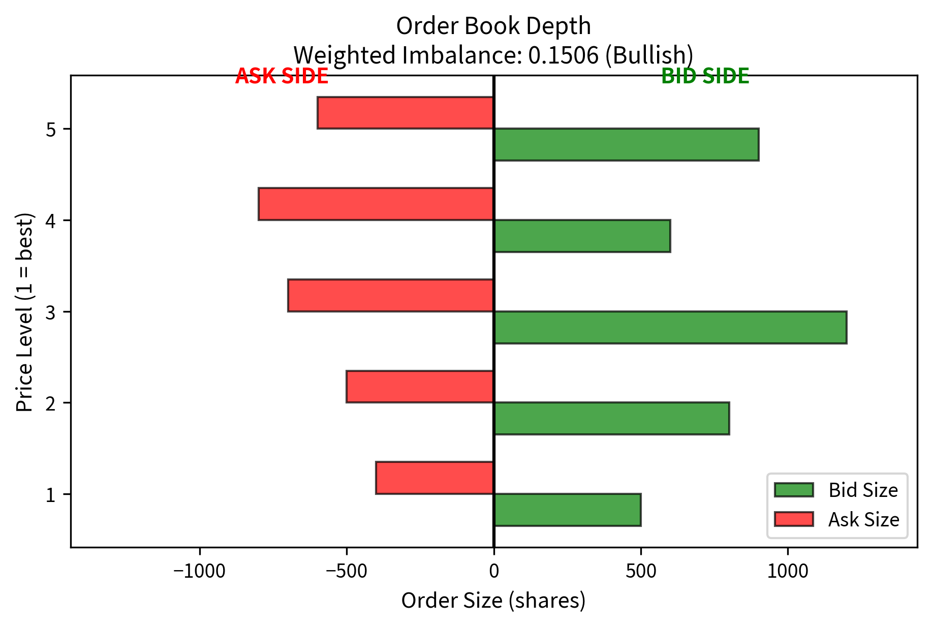
Order book imbalance: When there are substantially more bids than asks (or vice versa), prices tend to move in the direction of the imbalance.

Trade flow toxicity: Large, aggressive orders often precede continued price movement in the same direction. Detecting toxic flow allows you to widen spreads or reduce exposure.

Cross-market signals: Price movements in related instruments (futures, options, correlated stocks) can predict movements in the target instrument.

The weighted imbalance indicates directional pressure. The weighting gives more influence to the best prices (level 1 receives full weight, level 2 receives 50%, etc.), and this imbalance suggests short-term price pressure. Market makers would use this signal to adjust their quotes to lean against the expected move.

High-frequency trading has attracted significant regulatory attention. Understanding the regulatory landscape is essential for you if you're building or analyzing HFT systems.

Key regulations affecting HFT include:

• Regulation NMS (National Market System): In the U.S., Reg NMS requires that orders be routed to the exchange with the best price, creating the fragmented market structure that enables cross-market arbitrage. The rule also mandated that exchanges provide consolidated market data through the Securities Information Processor (SIP).

• Market Access Rule (SEC Rule 15c3-5): Requires broker-dealers to implement risk controls before providing market access to customers. This rule was enacted after the 2010 Flash Crash and targets potential risks from algorithmic and HFT trading.

• MiFID II (Markets in Financial Instruments Directive): This European regulation requires algorithmic trading firms to implement specific risk controls, maintain records of all orders and executions, and notify regulators of their algorithmic trading activities.

Several HFT practices have attracted criticism and regulatory scrutiny:

Controversial practices include:

• Quote stuffing: Submitting and immediately canceling large numbers of orders to slow down competitors' systems or create confusion in the order book. Most exchanges now charge fees for excessive order cancellations.

• Spoofing and layering: Placing orders with the intent to cancel before execution, creating a false impression of supply or demand. This practice is illegal under the Dodd-Frank Act.

• Front-running: In the traditional sense, trading ahead of customer orders is illegal. However, the ability of HFT firms to react faster to public information raises questions about whether their speed advantage constitutes an unfair practice.

The analysis shows a high cancel rate and order-to-trade ratio. High cancel rates are characteristic of legitimate market making activity, where firms continuously update quotes as conditions change, resulting in many cancellations. However, since this cancel rate exceeds the regulatory threshold, it may attract scrutiny for potential quote stuffing, despite potentially being legitimate market making behavior.

The key parameters for order-to-trade ratio analysis are:

• orders_submitted: Total number of orders sent to the market, including both executed and canceled orders.
• orders_executed: Number of orders that resulted in trades, a subset of submitted orders.
• cancel_rate: Fraction of orders canceled before execution (0 to 1), where high values may indicate quote stuffing.
• order_to_trade_ratio: Ratio of submitted orders to executed trades, a common metric for regulatory monitoring.
• regulatory_threshold: Cancel rate threshold triggering regulatory scrutiny (typically 0.90), which varies by jurisdiction.

HFT has fundamentally changed market dynamics, with both positive and negative effects.

Positive contributions include:

• Improved liquidity: HFT market makers provide continuous quotes across many securities and market conditions, reducing bid-ask spreads for all market participants. Since HFT became prevalent, spreads have declined dramatically. Academic research estimates that spreads for liquid securities have narrowed by 50% or more, with particularly active securities seeing even greater improvements.

• Price efficiency: By quickly arbitraging price discrepancies, HFT helps ensure that the same security trades at similar prices across venues, improving market efficiency.

• Lower transaction costs: Tighter spreads and improved price discovery have reduced trading costs for all market participants.

Negative effects and risks include:

• Flash crashes: On May 6, 2010, the Dow Jones Industrial Average dropped nearly 1,000 points (about 9%) in minutes before recovering. The event was triggered by a large sell order that destabilized HFT market makers, who withdrew liquidity en masse.

• Liquidity illusion: HFT liquidity can disappear instantly during stress, leaving markets illiquid precisely when liquidity is most needed. The 2010 Flash Crash and subsequent events demonstrated this vulnerability.

• Arms race costs: The resources devoted to achieving marginal speed improvements (microwave towers, submarine cables, FPGA development) represent significant social costs with debatable benefits.

The simulation demonstrates a flash crash scenario. Starting from the initial price, the price crashed significantly, representing a large maximum drawdown. During the crash, the number of active market makers dropped substantially as volatility and inventory limits triggered risk controls. This withdrawal of liquidity amplified price movements, creating a feedback loop where volatility caused liquidity withdrawal, which increased volatility further. The recovery began only when volatility subsided and market makers gradually returned to the market.

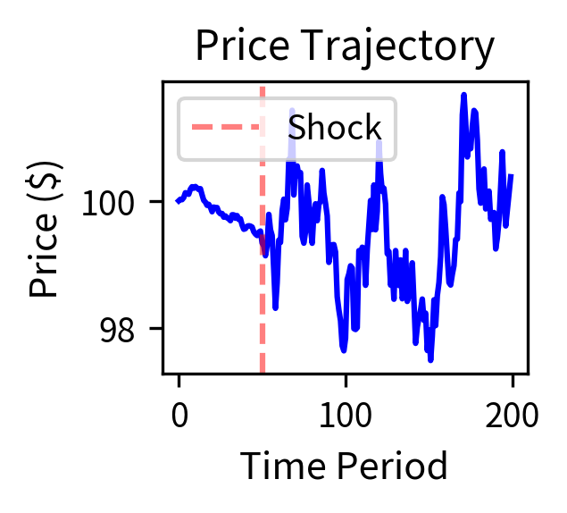
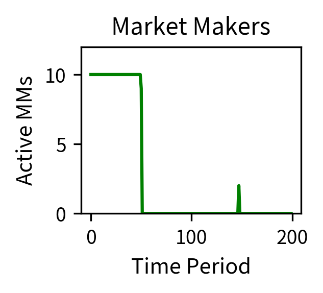
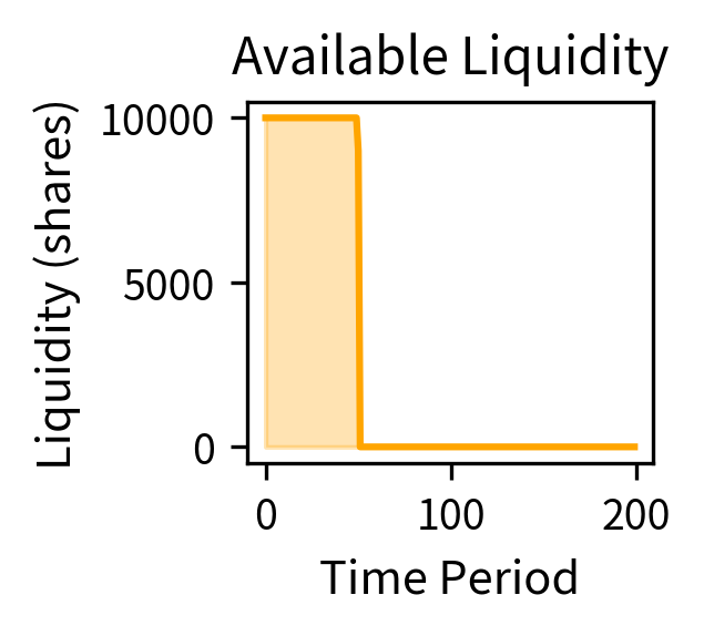
The simulation illustrates the feedback loop that creates flash crashes: an initial shock causes price volatility, which triggers market maker risk limits, leading to liquidity withdrawal, which amplifies price movements further. The recovery occurs only when volatility subsides and market makers gradually return.

High-frequency trading represents a fascinating intersection of finance, technology, and economics, but it faces significant challenges and raises important questions about market structure.

The competitive dynamics of HFT create a winner-take-most environment where profit margins continuously compress. Strategies that generated substantial returns a decade ago may now be marginally profitable or entirely unprofitable due to increased competition and market efficiency. This intense competition drives continuous investment in technology, leading to diminishing returns for market participants while potentially benefiting end investors through tighter spreads.

The infrastructure requirements for competitive HFT have created significant barriers to entry. If you're launching a new HFT firm, you must invest millions of dollars in co-location, direct data feeds, and specialized hardware before generating a single dollar of trading profit. This has led to consolidation in the industry, with a relatively small number of firms dominating trading volume, while the social value of these investments (resources devoted to shaving microseconds off transmission times) is debated.

Regulatory uncertainty remains a significant concern. Practices that are legal today may be prohibited in the future as regulators continue to study the effects of HFT on market quality and implement new rules to address emerging concerns. The 2010 Flash Crash prompted significant regulatory changes, and future events could trigger additional restrictions.

The adversarial relationship between HFT firms and other market participants creates an ongoing arms race. Institutional investors develop execution algorithms to minimize their footprint and avoid detection by HFT predators, while HFT firms develop increasingly sophisticated methods to detect and trade ahead of large orders. This cat-and-mouse game absorbs resources on both sides.

Despite these concerns, HFT has demonstrably improved some aspects of market quality. Bid-ask spreads are narrower than they were in the pre-HFT era, transaction costs have declined, and prices are more efficient. Whether these benefits justify the costs and risks of HFT is an ongoing debate among academics, regulators, and market participants.

The next chapter on Machine Learning Techniques for Trading examines how machine learning and artificial intelligence are transforming strategy development, building on the high-frequency trading foundations covered here. Many HFT firms have been early adopters of machine learning, using neural networks and reinforcement learning to optimize their strategies in ways that would have been impossible with traditional quantitative methods.

This chapter examined high-frequency trading and latency arbitrage, strategies that exploit tiny price discrepancies at enormous scale and extreme speeds.

The key economic insight of HFT is that small, consistent profits compound to substantial returns when executed at massive scale. Strategies earning fractions of a penny per trade can generate millions in annual profits through millions of daily executions.

Cross-market arbitrage exploits price discrepancies for the same or equivalent securities across different venues. Whether you're doing exchange arbitrage (same stock, different exchanges), ETF arbitrage (ETF vs. underlying basket), or futures-spot arbitrage, the principle is the same: buy cheap, sell expensive, and profit from the spread minus transaction costs.

Latency arbitrage exploits the time it takes for information to propagate across markets. By positioning technology closer to exchange matching engines and using faster communication channels, traders can react to price changes before competitors and capture predictable price adjustments.

The technology infrastructure of HFT includes co-location services that place servers adjacent to exchange matching engines, direct market data feeds that deliver information faster than consolidated feeds, FPGA-based systems that process data in microseconds, and optimized networks that minimize every source of delay.

The competitive dynamics create winner-take-most outcomes where being slightly faster captures most available profits. This drives continuous investment in speed improvements, creating an arms race with arguably diminishing social returns.

Regulatory considerations include requirements for risk controls, prohibitions on manipulative practices like spoofing and quote stuffing, and ongoing debate about whether HFT contributes to market stability or creates systemic risks.

The market impact of HFT includes positive effects (tighter spreads, improved price efficiency, lower transaction costs) alongside risks such as flash crashes, liquidity withdrawal during stress, and the potential for technological arms races to absorb resources without proportionate social benefits. Understanding these dynamics is essential for anyone working in modern financial markets, whether as a participant, regulator, or observer.

Ready to test your understanding? Take this quick quiz to reinforce what you've learned about high-frequency trading and latency arbitrage.