

Learn commodity futures pricing with cost of carry models, convenience yield, contango and backwardation analysis, and optimal hedging strategies.
Choose your expertise level to adjust how many terms are explained. Beginners see more tooltips, experts see fewer to maintain reading flow. Hover over underlined terms for instant definitions.
Commodity Markets and Futures
Commodity markets are among the oldest financial markets in human history. Long before stock exchanges existed, merchants traded contracts for future delivery of wheat, rice, and spices. The Dojima Rice Exchange in Osaka, Japan, established in 1697, is often cited as the first organized futures market. Today, commodity markets facilitate the trading of physical goods ranging from crude oil and natural gas to gold, copper, wheat, and coffee.
What makes commodity markets fascinating from a quantitative perspective is their connection to the physical world. Unlike a stock, which represents an abstract claim on future cash flows, a barrel of crude oil is a tangible object that must be stored, transported, and eventually consumed. This physical nature introduces unique pricing dynamics that don't exist in purely financial markets. Storage costs, transportation logistics, production seasonality, and the inherent value of having physical inventory on hand all influence commodity prices in ways that require specialized models to understand.
Futures contracts are the primary instruments used to trade commodities. A futures contract obligates the buyer to purchase, and the seller to deliver, a specific quantity of a commodity at a predetermined price on a specified future date. These standardized contracts trade on organized exchanges, providing liquidity, price transparency, and the ability to manage price risk. Understanding how futures prices relate to current spot prices, and why these relationships change over time, is essential for anyone working in commodity trading, risk management, or portfolio management.
Types of Commodity Markets
Commodity markets are typically organized into three major categories: energy, metals, and agricultural products. Each category has distinct characteristics that affect trading patterns, price behavior, and the types of participants involved.
Energy Commodities
Energy commodities include crude oil, natural gas, heating oil, gasoline, and increasingly, electricity and carbon credits. Crude oil is the most actively traded commodity in the world, with benchmarks like West Texas Intermediate (WTI) and Brent Crude serving as global price references.
Energy markets exhibit several distinctive features:
- Geopolitical sensitivity: Oil and gas prices respond sharply to geopolitical events, OPEC decisions, and regional conflicts in producing regions.
- Demand seasonality: Natural gas and heating oil show strong seasonal patterns due to heating demand in winter months.
- Infrastructure constraints: Pipeline capacity, refinery utilization, and storage availability create localized price differentials.
- Production decline: Oil and gas wells have declining production curves, requiring continuous investment in new exploration and development.
Metals
Metals divide into precious metals (gold, silver, platinum, palladium) and industrial metals (copper, aluminum, zinc, nickel, iron ore). These markets have fundamentally different drivers.
Precious metals, particularly gold, often serve as stores of value and inflation hedges. Gold prices respond to real interest rates, currency movements, and investor sentiment about economic uncertainty. Industrial metals, by contrast, are driven primarily by manufacturing activity and construction demand, making them sensitive to global economic growth, particularly in China.
Agricultural Commodities
Agricultural commodities encompass grains (wheat, corn, soybeans, rice), soft commodities (coffee, cocoa, sugar, cotton), and livestock (cattle, hogs). These markets exhibit the most pronounced seasonality due to harvest cycles and growing seasons.
Agricultural markets face unique supply-side risks:
- Weather dependence: Droughts, floods, and temperature extremes can dramatically affect crop yields.
- Biological constraints: Unlike industrial production, agricultural output cannot be easily scaled up in response to high prices.
- Perishability: Many agricultural products have limited shelf life, constraining storage options.
How Commodities Differ from Financial Assets
The physical nature of commodities creates fundamental differences from financial assets that profoundly affect pricing and trading strategies.
Storage Costs
Holding physical commodities incurs costs that don't exist for financial assets. Storing crude oil requires tank farms or ship charters. Storing grain requires silos with temperature and humidity control. Storing precious metals requires secure vaults and insurance. These storage costs are a critical component of futures pricing.
The cost of holding physical inventory over time, including warehousing fees, insurance, financing costs, and any losses due to spoilage or deterioration. Storage costs are typically expressed as a percentage of commodity value per unit time.
The Cost of Carry Model
When we think about the relationship between spot and futures prices, we must start with a fundamental question: why should a futures price differ from today's spot price at all? The answer lies in understanding what it means to hold a commodity over time. If you want to have a barrel of oil available in six months, you have two choices. You can either buy it today and store it until you need it, or you can buy a futures contract that guarantees delivery in six months. These two approaches must lead to economically equivalent outcomes; otherwise, arbitrageurs would exploit the difference until prices realign.
This insight forms the foundation of the cost of carry model, which establishes the theoretical relationship between spot and futures prices for storable commodities. The model recognizes that carrying physical inventory forward in time is not free. It costs money to finance the purchase, and it costs money to store the commodity safely.
For commodities that can be stored, the relationship between spot prices and futures prices follows the cost of carry model. If is the current spot price, then the theoretical futures price for delivery at time is:
where:
- : theoretical futures price
- : current spot price
- : risk-free interest rate
- : storage cost rate (continuous)
- : time to delivery
This formula captures two components of carrying inventory, and understanding each component illuminates why futures prices behave as they do:
- Financing cost: Capital tied up in inventory could earn the risk-free rate. When you buy a commodity and hold it, you forgo the interest you could have earned by investing that capital elsewhere. This opportunity cost accumulates continuously over time.
- Storage cost: Physical storage incurs direct costs. These include warehouse rental, insurance against damage or theft, and any costs associated with maintaining the commodity in deliverable condition.
To see why this relationship must hold, consider the simplest case: a commodity with no storage costs and no other carrying charges. In this scenario, the futures price would simply be:
where:
- : futures price
- : spot price
- : risk-free interest rate
- : time to delivery
This relationship arises from no-arbitrage arguments, a fundamental principle in financial economics. The logic is straightforward: if two strategies produce identical outcomes, they must cost the same amount today. If they don't, someone can make a guaranteed profit with no risk, which market forces will quickly eliminate.
Consider what happens if . In this case, an arbitrageur could earn a risk-free profit through the following steps:
- Borrow at rate to buy the spot commodity.
- Sell a futures contract at price .
- Hold the commodity until time .
- Deliver the commodity to settle the futures contract, receiving .
- Repay the loan, which has grown to .
The risk-free profit is . Notice that this profit requires no initial capital and involves no price risk, since both the selling price (fixed by the futures contract) and the repayment amount (determined by the loan terms) are known from the start. If the futures price were below this level, the reverse arbitrage (short selling spot, investing proceeds, buying futures) would apply, again generating risk-free profit. In either case, arbitrage activity pushes prices toward the theoretical relationship.
Convenience Yield
The cost of carry model as presented above predicts that futures prices should always exceed spot prices by the carrying costs. The logic seems airtight: holding inventory costs money, so the futures price must compensate for those costs. Yet in practice, we often observe the opposite: futures prices trading below spot prices. This phenomenon demands explanation, and the concept of convenience yield provides it.
The non-monetary benefit that accrues to holders of physical inventory. It represents the value of having immediate access to the commodity for production, consumption, or to meet unexpected demand. The convenience yield is implicit and cannot be directly observed; it must be inferred from the relationship between spot and futures prices.
To understand convenience yield intuitively, consider why someone might prefer to hold physical inventory even when futures contracts exist. The answer lies in the optionality that physical ownership provides. A futures contract obligates you to take delivery at a specific time, but it cannot help you if you need the commodity unexpectedly before that date. Physical inventory, by contrast, can be deployed immediately.
The convenience yield arises because holding physical inventory provides optionality that futures contracts do not. A refinery with crude oil in its tanks can respond immediately to a spike in gasoline demand. A manufacturer with copper inventory can fulfill urgent orders without supply chain delays. A farmer with grain stores can sell into local price spikes. This flexibility has value, and market participants are willing to accept lower returns on inventory holdings to maintain it. In effect, they are "paying" for the option to use the commodity immediately if needed.
Incorporating convenience yield into the cost of carry model modifies our pricing equation by adding a term that offsets carrying costs:
where:
- : futures price
- : spot price
- : risk-free rate
- : storage cost rate
- : convenience yield rate
- : time to delivery
The exponent represents the net cost of carrying the commodity forward, and understanding each component clarifies the economic forces at work:
- : the cost of carry (interest plus storage), which pushes futures prices up because holding inventory is expensive
- : the convenience yield benefit, which pushes futures prices down because holders of physical inventory receive valuable optionality
When convenience yield exceeds storage and financing costs (), futures prices will be below spot prices. The net cost of carry becomes negative, reflecting that the benefits of holding physical inventory outweigh the costs.
Inventory and the Convenience Yield Relationship
Having established that convenience yield represents the value of holding physical inventory, we now turn to a crucial question: what determines the magnitude of this yield? Intuition suggests that the answer relates to scarcity. When inventory is plentiful, having a bit more provides little additional security, since you can easily obtain more from the market. When inventory is scarce, however, each additional unit becomes increasingly valuable because the risk of running out rises.
The convenience yield is not constant; it varies with inventory levels. When inventories are abundant, the marginal convenience yield of additional inventory is low, as there's little risk of stockouts. When inventories are scarce, the convenience yield rises sharply because having physical supply becomes increasingly valuable. This relationship has important implications for futures pricing, as it means the term structure of futures prices responds dynamically to supply conditions.
This relationship was formalized in the theory of storage developed by economists studying commodity markets. The theory models convenience yield as a decreasing function of inventory:
where:
- : convenience yield
- : inventory level
- : yield function relating inventory to convenience
- : yield decreases as inventory increases
The negative derivative captures the economic intuition: as inventory grows, the marginal value of additional stock diminishes. At very high inventory levels, convenience yield approaches zero, and futures prices reflect pure carrying costs. The market has so much inventory that no one worries about shortages, so the optionality of immediate access provides little value. At very low inventory levels, convenience yield can be substantial, potentially exceeding carrying costs. In these situations, market participants place high value on having physical supply available, and this urgency is reflected in spot prices that exceed futures prices.
Seasonality in Production and Consumption
Many commodities exhibit predictable seasonal patterns in either supply or demand. Agricultural commodities have obvious harvest cycles: corn and soybeans are harvested in autumn in the Northern Hemisphere, while wheat has winter and spring varieties with different harvest times.
Energy commodities show demand seasonality: heating oil and natural gas demand peaks in winter, while gasoline demand peaks in summer driving season. These seasonal patterns create predictable variations in spot-futures price relationships throughout the year.
Futures Pricing: Contango and Backwardation
Having developed the theoretical framework for understanding spot-futures relationships, we can now examine how these relationships manifest in actual market conditions. The term structure of futures prices, which shows how futures prices vary across different delivery months, reveals important information about market conditions and expectations. By observing whether futures prices rise or fall as we look further into the future, we can infer information about storage costs, convenience yields, and market participants' views on future supply and demand.
Contango
When markets are well-supplied and convenience yield is low, the cost of carry dominates the pricing relationship. Futures prices exceed spot prices because someone buying for future delivery must compensate the counterparty for the costs of storing and financing the commodity until the delivery date. This market condition has a specific name.
A market condition where futures prices are higher than the current spot price, and longer-dated futures are more expensive than near-term futures. Contango reflects positive net carrying costs and typically occurs when storage capacity is available and inventories are adequate.
In contango, the futures curve slopes upward, meaning prices increase as we look at contracts with later delivery dates. Mathematically, this relationship can be expressed as an ordering of prices across maturities:
where:
- : futures prices for maturities
- : spot price
Contango is the "normal" condition predicted by the simple cost of carry model when convenience yield is low. The upward slope compensates holders of physical inventory for their storage costs. Without this compensation, no rational actor would store commodities for future sale. A market in contango provides incentives for storage: traders can buy spot, sell futures, and earn the spread minus storage costs. This cash-and-carry trade is one of the fundamental arbitrage strategies in commodity markets.
Backwardation
When supply conditions tighten and convenience yield rises, a different market structure emerges. If the value of holding physical inventory exceeds the costs of storage and financing, the theoretical futures price falls below the spot price. This creates an inverted term structure.
A market condition where futures prices are below the current spot price, and longer-dated futures are cheaper than near-term futures. Backwardation reflects high convenience yield, typically associated with supply scarcity or strong immediate demand.
In backwardation, the futures curve slopes downward, with prices declining as delivery dates extend further into the future:
where:
- : futures prices for maturities
- : spot price
Backwardation signals tight supply conditions. When inventories are low and immediate demand is strong, spot prices rise relative to futures. The market is "paying" for immediate delivery because the commodity is needed now, not later. This premium for immediacy reflects the high convenience yield that holders of physical inventory enjoy. Producers can lock in attractive prices by selling futures, while consumers face a premium for immediate supply.
Measuring the Term Structure
To quantify the relationship between spot and futures prices, traders and analysts use several standard measures. These metrics provide a common language for discussing market conditions and comparing opportunities across different commodities and time periods.
The basis measures the relationship between spot and futures prices:
where:
- : spot price
- : futures price
A positive basis indicates backwardation (spot above futures), while a negative basis indicates contango (futures above spot). The basis is a crucial metric for hedgers because it directly affects the cost or benefit of maintaining hedged positions. Changes in the basis represent a source of risk that even perfectly hedged positions must bear.
The calendar spread measures the price difference between two futures contracts with different delivery months:
where:
- : price of near-term contract
- : price of far-term contract
Calendar spreads are particularly useful if you want to take views on changes in market structure without exposure to outright price direction. If you believe that supply conditions will tighten, you can buy the spread, profiting if backwardation deepens, without betting on whether overall prices will rise or fall.
The roll yield captures the return from maintaining a futures position as contracts approach expiration and must be rolled into longer-dated contracts. In backwardation, roll yield is positive because investors sell expensive near-term contracts and buy cheaper far-term contracts. In contango, roll yield is negative. This concept is essential for understanding the performance of commodity index investments, which must continuously roll their futures positions.
Market Participants
Commodity markets bring together participants with diverse objectives, creating the liquidity and price discovery that makes these markets function.
Producers
Producers are entities that extract, grow, or manufacture commodities. Oil and gas companies, mining firms, and farmers fall into this category. Producers have natural long exposure to commodity prices: when prices rise, their revenues increase; when prices fall, their revenues decline.
Producers use futures markets primarily to hedge their price risk. A wheat farmer might sell futures contracts before harvest to lock in a price, eliminating uncertainty about revenue regardless of where prices move by harvest time. An oil producer might sell crude oil futures to guarantee cash flows needed to service debt or fund capital expenditures.
Consumers
Consumers are entities that use commodities as inputs to production. Airlines consume jet fuel, utilities consume natural gas, and food processors consume agricultural products. Consumers have natural short exposure to commodity prices: rising prices increase their costs.
Consumers hedge by buying futures contracts to lock in input costs. An airline might buy jet fuel futures to establish predictable operating costs for budget planning. A cereal manufacturer might buy corn futures to fix ingredient costs before setting retail prices.
Speculators
Speculators have no underlying exposure to physical commodities. They trade futures purely to profit from anticipated price movements. While often viewed negatively in public discourse, speculators provide essential services to commodity markets:
- Liquidity: Speculators enable hedgers to enter and exit positions at competitive prices
- Price discovery: Speculative trading incorporates diverse information and views into prices
- Risk transfer: Speculators absorb risks that hedgers want to shed
Speculators include individual traders, hedge funds, commodity trading advisors (CTAs), and proprietary trading firms. They employ diverse strategies ranging from fundamental analysis of supply and demand to technical trading based on price patterns to quantitative models exploiting statistical relationships.
Arbitrageurs
Arbitrageurs seek to profit from pricing inconsistencies across markets or contracts. In commodity markets, common arbitrage strategies include:
- Cash-and-carry arbitrage: Exploiting mispricing between spot and futures by buying physical commodity and selling futures
- Calendar spread arbitrage: Trading price discrepancies between different futures months
- Geographic arbitrage: Exploiting price differences for the same commodity in different locations
Arbitrage activity keeps prices aligned across markets and ensures that theoretical pricing relationships hold approximately in practice.
Hedging with Commodity Futures
Hedging is the primary economic function of futures markets. By taking offsetting positions in futures, commercial participants can transfer price risk to others willing to bear it.
The Basic Hedge
Consider a farmer expecting to harvest 50,000 bushels of corn in six months. Current corn futures for delivery in six months trade at $4.50 per bushel. The farmer can lock in this price by selling 10 futures contracts (each contract covers 5,000 bushels).
If corn prices fall to $4.00 at harvest
- The farmer receives $4.00 per bushel in the physical market
- The futures position profits $0.50 per bushel ($4.50 - $4.00)
- Net effective price: $4.50 per bushel
If corn prices rise to $5.00 at harvest
- The farmer receives $5.00 per bushel in the physical market
- The futures position loses $0.50 per bushel ($4.50 - $5.00)
- Net effective price: $4.50 per bushel
In both scenarios, the hedge locks in the $4.50 price. The farmer sacrifices upside potential in exchange for downside protection.
Hedge Ratio and Basis Risk
Perfect hedges are rare in practice. The commodity being hedged may differ from the commodity underlying the futures contract in grade, quality, location, or timing of delivery. Even when the commodity matches perfectly, spot and futures prices do not move in lockstep. These imperfections mean that hedgers must carefully consider how large a futures position to take relative to their spot exposure.
To determine the optimal hedge ratio , we seek to minimize the variance of the hedged portfolio's value changes. This is a classic optimization problem: we want to find the position size that most effectively reduces risk. The approach begins by writing out the variance of the hedged position and then finding the value of that minimizes this variance.
Consider a position that is long the spot commodity and short futures contracts. The change in the portfolio's value equals the change in spot price minus times the change in futures price. The variance of this hedged position can be expanded using standard properties of variance:
where:
- : variance of the hedged position value changes
- : standard deviation of spot price changes
- : standard deviation of futures price changes
- : hedge ratio
- : correlation between spot and futures price changes
This expression decomposes risk into three parts, each with a clear economic interpretation:
- : the variance of the unhedged spot position, representing the baseline risk we seek to reduce
- : the variance added by the futures position, which increases with the square of the hedge ratio
- : the covariance term that reduces total risk, provided , by capturing the offsetting movements between spot and futures
The key insight is that the third term provides the risk reduction we seek. When spot prices rise, futures prices tend to rise as well (assuming positive correlation), so the short futures position generates losses that offset the gains from the long spot position. The optimization challenge is to balance the risk reduction from the covariance term against the additional variance introduced by the futures position itself.
To find the minimum variance, we take the derivative with respect to , set it to zero, and solve for . This standard calculus technique identifies the point where the variance function reaches its minimum:
where:
- : optimal hedge ratio
- : correlation between spot and futures price changes
- : standard deviation of spot price changes
- : standard deviation of futures price changes
This formula shows that the optimal hedge depends on two factors: the strength of the relationship between spot and futures prices, as captured by the correlation , and the relative volatility of the two instruments, expressed as the ratio . If futures are more volatile than the spot price, a smaller futures position is needed to offset the risk, because each futures contract "punches above its weight" in terms of risk contribution. If the correlation is imperfect, the hedge ratio scales down accordingly, since the offsetting effect is weaker.
The risk that the spot-futures price relationship changes unexpectedly during the hedge period. Basis risk arises because the physical commodity being hedged may not match the futures contract specification exactly (grade, location, timing), and because the basis is influenced by supply-demand factors that can shift.
Basis risk means that even a hedged position retains some price exposure. The hedge converts outright price risk into basis risk, which is typically smaller and more predictable, but not zero. A wheat farmer hedging with Chicago wheat futures still faces the risk that local basis conditions change between the time the hedge is placed and the time the physical grain is sold.
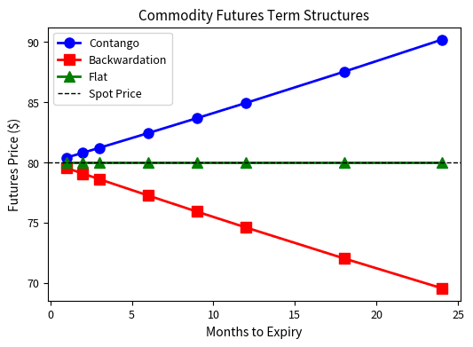
Analyzing Futures Term Structure
Let's build tools to analyze commodity futures term structures and visualize contango and backwardation conditions.
We'll create a function to generate theoretical futures curves under different market conditions:
Now let's visualize the three term structure scenarios:

The basis values confirm our term structure shapes. In contango, the negative basis reflects futures prices above spot. In backwardation, the positive basis shows spot prices exceeding futures.
Calculating Roll Yield
Roll yield is the return generated when rolling futures positions forward. Let's calculate the annualized roll yield for different term structure conditions:

The roll yield calculations highlight why commodity investors care deeply about term structure. In persistent contango, continuously rolling long futures positions erodes returns. In persistent backwardation, roll yield adds to returns.
Hedging Example: Crude Oil Producer
Let's work through a complete hedging example for an oil producer seeking to lock in prices for future production.


The visualization demonstrates the core trade-off of hedging. The producer sacrifices the potential to benefit from price increases in exchange for protection against price declines. The hedge transforms uncertain future revenue into a known quantity.
Calculating the Optimal Hedge Ratio
When the commodity being hedged doesn't perfectly match the futures contract, we need to calculate the optimal hedge ratio using historical price data:

The optimal hedge ratio of approximately 0.74 indicates that the hedge requires fewer futures contracts than a naive one-to-one hedge. This occurs because futures prices are more volatile than spot prices in our simulated data, so fewer contracts are needed to offset the same dollar risk.
Hedge Effectiveness
We can measure how well the hedge performs by comparing the variance of unhedged and hedged positions:


The hedge effectiveness of approximately 85% indicates that the optimal hedge removes most, but not all, price risk. The remaining 15% represents basis risk arising from imperfect correlation between the spot commodity and the futures contract used for hedging.
Key Parameters
The key parameters for analyzing futures pricing and hedging are:
- spot: Current market price of the physical commodity for immediate delivery.
- time_to_expiry: Time remaining until the futures contract matures, typically expressed in years.
- risk_free_rate: The theoretical return on an investment with zero risk, used for discounting future cash flows.
- storage_cost: The cost of holding physical inventory, expressed as a percentage of the commodity's value.
- convenience_yield: The implied benefit of holding physical inventory rather than futures, reflecting supply scarcity.
- hedge_ratio: The size of the futures position relative to the spot exposure, used to minimize variance.
Limitations and Practical Considerations
Commodity futures trading involves complexities that theoretical models often simplify or ignore. Understanding these limitations is essential for practitioners.
The cost of carry model assumes frictionless markets where storage can be arranged at any scale, physical delivery is straightforward, and arbitrage can be executed instantly. In reality, storage capacity is finite and concentrated among a limited number of firms. During periods of oversupply, such as the oil market collapse in early 2020, storage constraints can cause dramatic price dislocations. WTI crude oil futures briefly traded negative in April 2020 because the market faced a situation where physical delivery was required but storage was unavailable at any price.
Convenience yield, while conceptually elegant, cannot be directly observed or measured. It must be inferred from the difference between actual futures prices and what the pure cost of carry model predicts. This makes convenience yield somewhat circular in practice: we define it as whatever residual is needed to reconcile observed prices with theory. Moreover, convenience yield varies not just with aggregate inventory but with who holds the inventory, where it is located, and what the holder's specific needs are.
Liquidity in commodity futures markets is heavily concentrated in near-term contracts. While the front-month crude oil contract might trade millions of contracts daily, contracts with delivery dates two or three years out may trade only thousands. This creates challenges for hedgers seeking protection over longer horizons and can introduce execution costs and slippage that erode hedge effectiveness.
Physical delivery mechanics create operational risks. Most financial participants roll positions before expiration to avoid delivery, but miscalculations can lead to the obligation to accept or deliver physical commodities. The infrastructure, logistics, and documentation requirements for physical settlement are substantial, and many trading firms have learned expensive lessons by inadvertently holding positions into the delivery period.
Summary
This chapter explored commodity markets and futures, focusing on the unique characteristics that distinguish commodities from financial assets. The physical nature of commodities introduces storage costs, convenience yield, and delivery logistics that fundamentally affect pricing relationships.
The cost of carry model provides the theoretical framework for understanding futures pricing:
where:
- : futures price
- : spot price
- : risk-free rate
- : storage cost rate
- : convenience yield rate
- : time to delivery
When convenience yield is low relative to carrying costs, markets exhibit contango with upward-sloping futures curves. When convenience yield is high due to supply scarcity, markets exhibit backwardation with downward-sloping curves. The term structure provides valuable information about market conditions and expectations.
Market participants include producers and consumers who hedge physical price exposure, speculators who provide liquidity and absorb risk, and arbitrageurs who keep prices aligned across markets. The optimal hedge ratio is calculated as:
where:
- : optimal hedge ratio
- : correlation between spot and futures
- : volatilities of spot and futures
This minimizes variance of the hedged position, though basis risk ensures that some exposure remains.
Understanding these fundamentals prepares you for analyzing commodity markets quantitatively, whether for trading, risk management, or portfolio construction. The interplay between physical market fundamentals and financial derivatives creates rich dynamics that reward careful analysis and disciplined approach to model limitations.
Quiz
Ready to test your understanding? Take this quick quiz to reinforce what you've learned about commodity markets and futures pricing.

Comments