

Master volatility as an asset class. Learn delta hedging, variance swaps, dispersion trading, and VIX strategies to exploit implied versus realized volatility.
Choose your expertise level to adjust how many terms are explained. Beginners see more tooltips, experts see fewer to maintain reading flow. Hover over underlined terms for instant definitions.
Volatility Trading and Arbitrage Strategies
Volatility is more than just a parameter in option pricing models; it is a tradeable asset class in its own right. While you might focus on predicting the direction of asset prices, you take positions on the magnitude of future price movements, regardless of direction. This distinction opens up an entirely different dimension of market opportunity.
The appeal of volatility trading stems from several observations. First, as we explored in Part III's discussion of implied volatility and the volatility smile, implied volatility extracted from option prices often differs systematically from subsequently realized volatility. This persistent gap, known as the volatility risk premium, creates opportunities for those who can model and harvest it. Second, volatility exhibits mean-reverting behavior and clustering effects, as we saw when studying GARCH models in Part III, Chapter 18. These statistical properties make volatility more predictable than price returns in certain respects. Third, volatility positions can provide portfolio diversification benefits, as volatility tends to spike during market stress when traditional assets decline.
This chapter develops the tools and strategies for trading volatility. We begin by examining the instruments available, from vanilla options to VIX futures and variance swaps, before diving into delta hedging strategies that isolate pure volatility exposure. We then explore volatility arbitrage, where you exploit mispricings between implied and realized volatility, and dispersion trading, which capitalizes on the relationship between index volatility and constituent volatility. Throughout, we emphasize the substantial risks involved, particularly for strategies that are short volatility.
Volatility as an Asset Class
Before examining specific strategies, we need to understand what it means to trade volatility and the instruments available for doing so.
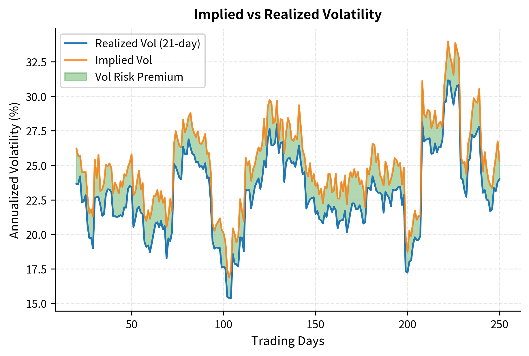
Implied Versus Realized Volatility
Recall from Part III, Chapter 8 that implied volatility () is the volatility level that, when plugged into the Black-Scholes formula, produces the observed market price of an option. It represents the market's expectation of future volatility over the option's life, plus any risk premium. Realized volatility (), in contrast, is the actual volatility that materializes over a given period, typically calculated as the annualized standard deviation of log returns.
Distinguishing between these two measures is fundamental to volatility trading. Implied volatility is forward-looking: it captures what market participants collectively believe will happen to the underlying asset's price movements over the life of the option. This belief is embedded in the prices they are willing to pay for options. Realized volatility, on the other hand, is backward-looking: it measures what actually occurred in the market during a specific historical period. These two measures are rarely equal. Markets must form expectations about the future under uncertainty, and those expectations can systematically differ from what eventually transpires.
The relationship between these two quantities drives most volatility trading strategies:
- When : Options are "expensive" relative to the volatility that actually occurs. Selling options and delta-hedging can be profitable.
- When : Options are "cheap" relative to realized moves. Buying options and delta-hedging captures the volatility differential.
In the first scenario, market participants overestimated future price movements. They paid a premium for protection or speculation that was larger than justified by the actual market conditions. If you recognize this overpricing, you can sell options, collect the inflated premium, and hedge away the directional exposure, profiting from the difference between what was expected and what occurred. In the second scenario, market participants underestimated future volatility. If you buy these cheap options and manage the directional risk, you profit when the market moves more than expected.
The Volatility Risk Premium
The volatility risk premium (VRP) is the systematic tendency for implied volatility to exceed subsequently realized volatility. This premium exists because investors are generally willing to pay extra for portfolio protection during market declines. Just as insurance premiums exceed expected claims to compensate insurers for bearing tail risk, option premiums include compensation for volatility sellers who bear the risk of extreme moves.
Investor behavior and market structure drive the volatility risk premium. Most institutional investors hold long equity portfolios, and their primary concern during market stress is downside protection. When uncertainty increases, these investors bid up the prices of put options and other hedging instruments, driving implied volatility above the level that purely reflects expected realized volatility. Volatility sellers, who step in to provide this insurance, demand compensation for taking on the risk that markets could move more violently than anticipated. This compensation manifests as the persistent gap between implied and realized volatility.
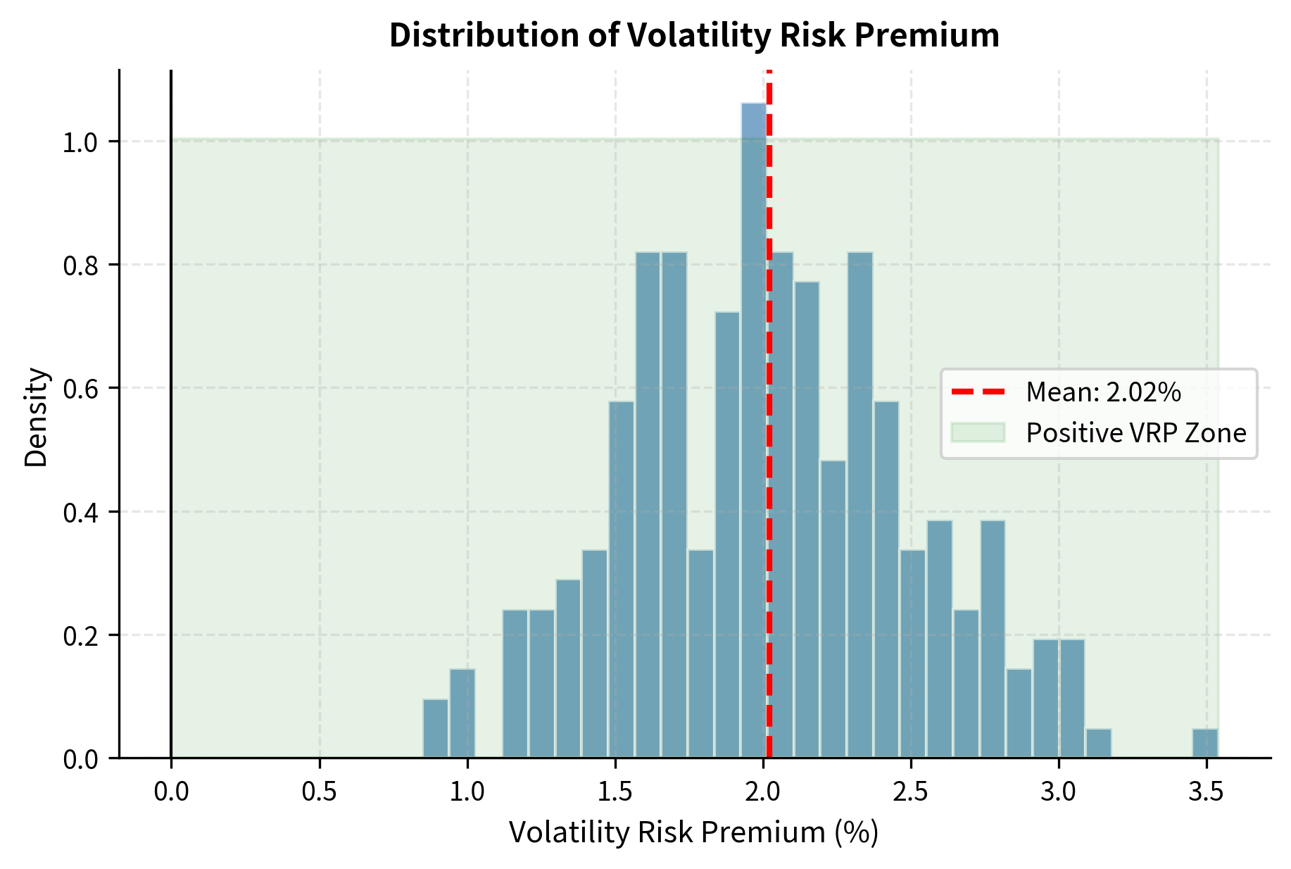
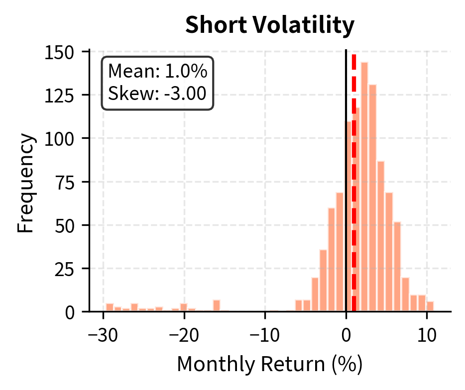
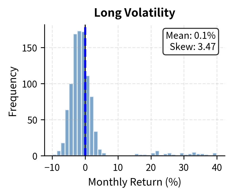
A positive average volatility risk premium does not make selling volatility a free lunch. The distribution of returns from short volatility strategies is highly negatively skewed, with small gains most of the time punctuated by occasional large losses during volatility spikes.
Instruments for Trading Volatility
You have several instruments at your disposal:
Options on Underlying Assets
The most direct way to gain volatility exposure is through options on stocks, indices, or ETFs. Buying straddles or strangles provides long volatility exposure, while selling them provides short volatility exposure. However, options also carry delta exposure to the underlying asset's direction, which must be managed.
VIX and Volatility Index Futures
The CBOE Volatility Index (VIX) measures the 30-day implied volatility of S&P 500 index options. VIX futures allow you to take positions on expected future levels of implied volatility. The VIX futures curve is typically in contango (upward sloping), meaning longer-dated futures trade at higher prices than spot VIX, creating a roll cost for long VIX positions.
Variance Swaps
A variance swap is an over-the-counter derivative that pays the difference between realized variance and a fixed strike variance. Unlike options, variance swaps provide pure exposure to realized volatility without any delta component. We will examine these in detail later in this chapter.
Volatility ETFs and ETNs
Products like VXX (short-term VIX futures ETN) and SVXY (inverse VIX ETF) provide retail-accessible volatility exposure. These products suffer from significant roll costs and are designed for short-term trading rather than buy-and-hold positions.
Delta-Hedged Option Strategies
The key to isolating pure volatility exposure from options is delta hedging. By continuously adjusting a hedge position in the underlying asset, you can neutralize directional exposure and focus exclusively on whether implied volatility overstates or understates realized volatility.
The Mechanics of Delta Hedging
Consider if we sell a call option with delta . To become delta-neutral, we buy shares of the underlying. As the underlying price moves and time passes, the option's delta changes. We must rebalance the hedge, buying more shares when delta increases and selling when delta decreases.
Delta hedging transforms an option position with directional and volatility exposure into a pure volatility bet. When you sell an option without hedging, your profit depends heavily on which way the underlying asset moves. But when you hedge away the directional exposure by holding offsetting shares, your profit depends only on whether the option was priced correctly relative to the actual volatility that materializes. This separation of concerns is what makes volatility trading possible as a distinct discipline.
A delta-neutral position has zero first-order sensitivity to small changes in the underlying price. For a portfolio of options and underlying shares, the position is delta-neutral when , where is the delta of each position and is the quantity.
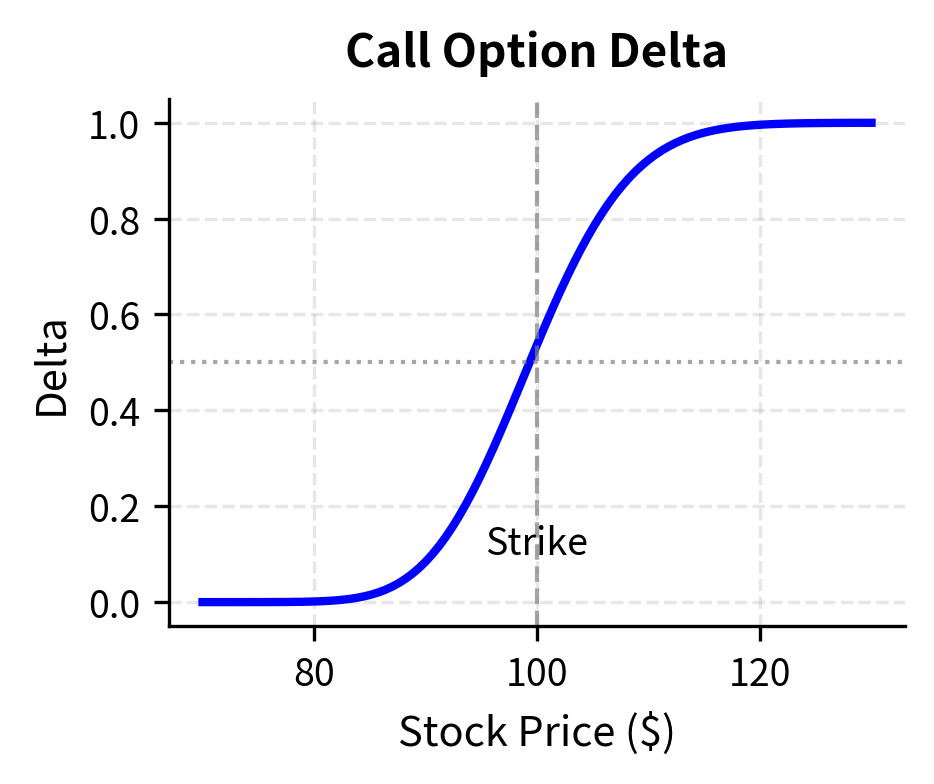
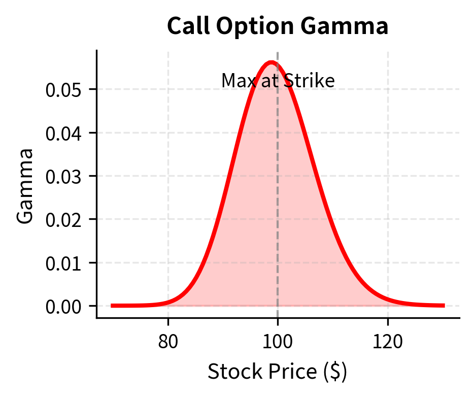
The positive delta indicates that the option price moves in the same direction as the underlying asset. To hedge a short call position (which has negative delta exposure), you must buy shares of the underlying asset to neutralize directional risk. The gamma value represents the curvature of the option price; a higher gamma requires more frequent rebalancing of the hedge ratio. Gamma tells us how quickly the delta changes as the underlying moves, and therefore how much trading activity will be required to maintain the hedge. Options near the money and close to expiration have the highest gamma, meaning they require the most active management.
P&L from Delta-Hedged Positions
The profit or loss from a delta-hedged option position comes from the interaction between the option's theta decay and the gamma-driven gains from rebalancing. To understand this relationship, we need to analyze how the value of a delta-hedged portfolio changes over time and with price movements.
We can derive the P&L dynamics by analyzing the change in value of the delta-hedged portfolio . Using a second-order Taylor expansion (Ito's Lemma):
where:
- : profit or loss over the time step
- : option value
- : option delta
- : option gamma
- : underlying asset price
- : realized volatility of the underlying asset
- : small time increment
- : option theta
This derivation shows the tension in delta-hedged option positions. The first step applies Ito's Lemma to express how the option value changes: it moves with time (theta), with the underlying price (delta times the price change), and with the square of the price change (half gamma times the squared move). When we subtract the hedge position's change in value, the delta terms cancel perfectly because that is exactly what the hedge is designed to do. What remains are the theta and gamma terms, which cannot be hedged away simultaneously.
For a delta-hedged long option position:
- Theta (): The option loses value due to time decay. This is a cost.
- Gamma (): When the underlying moves, the hedge position profits from rebalancing. This is a gain.
The key insight is that theta cost is determined by implied volatility (priced into the option), while gamma gains are determined by realized volatility (actual market moves). If realized volatility exceeds implied, gamma gains exceed theta costs, and the long volatility position profits. This is the essential mechanism of volatility trading: you are betting on whether the actual price movements will be larger or smaller than what the option price assumed.
The theta of an option represents the daily cost of maintaining the position, and this cost is higher when implied volatility is higher because a higher implied volatility means a more expensive option that has more time value to decay. The gamma gains, conversely, depend on how much the underlying actually moves. When the underlying makes a large move, a long gamma position benefits because the delta has changed, and the hedge needs rebalancing at favorable prices. If these actual moves are consistently larger than what was priced in, the rebalancing gains exceed the time decay costs.
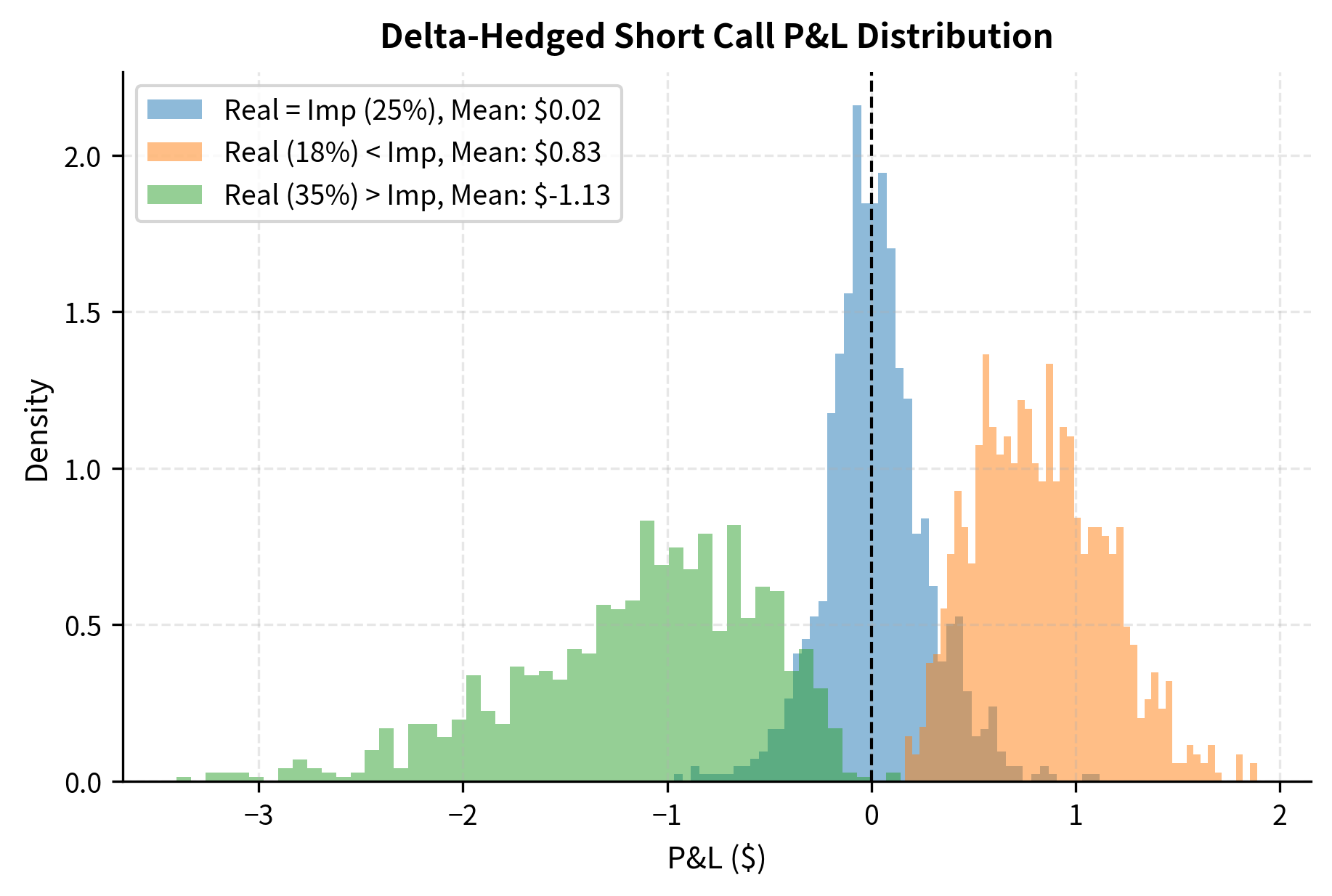
The simulation confirms our theoretical expectation: when realized volatility is lower than implied, the short volatility position profits from collecting more theta than it loses to gamma. When realized volatility exceeds implied, the position loses money as gamma costs exceed theta gains. Notice also that even when realized and implied volatility are equal, there is dispersion in outcomes. This variance arises because while the average gamma gain equals the average theta loss, the actual path matters, and some paths will be more favorable than others purely by chance.
Gamma Scalping
Gamma scalping is a trading technique that attempts to profit from the gamma of a long option position. If you are long gamma (long options), you benefit when the underlying makes large moves in either direction. By rebalancing delta frequently, you "lock in" gains from these moves.
When you are long gamma and the stock rises, your delta increases. You are effectively longer the stock at higher prices. By selling some shares to rebalance to delta-neutral, you capture a profit. Similarly, when the stock falls, your delta decreases, and by buying shares at lower prices, you profit again.
To understand why this works, consider the mechanics of the hedge adjustment. When you are long a call option and the stock rises, your call option increases in value, but so does its delta. If you started with a delta-neutral position, you are now slightly long the market because your call is more sensitive to further moves. To restore neutrality, you sell shares at the current higher price. If the stock subsequently falls back, you will need to buy shares again at the lower price. You have effectively sold high and bought low, locking in a trading profit. This profit comes from the convexity of the option's payoff, which is measured by gamma.
You must weigh these gamma gains against theta decay. A long gamma position pays theta every day as the option loses time value. If the stock does not move enough to generate sufficient rebalancing profits, the theta costs will dominate and the position will lose money. This is why gamma scalping is only profitable when realized volatility exceeds implied volatility: the moves must be large enough and frequent enough to offset the daily time decay.
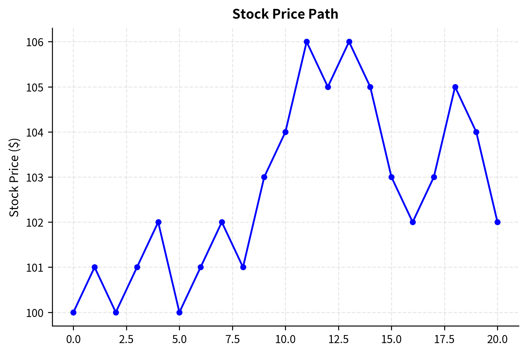
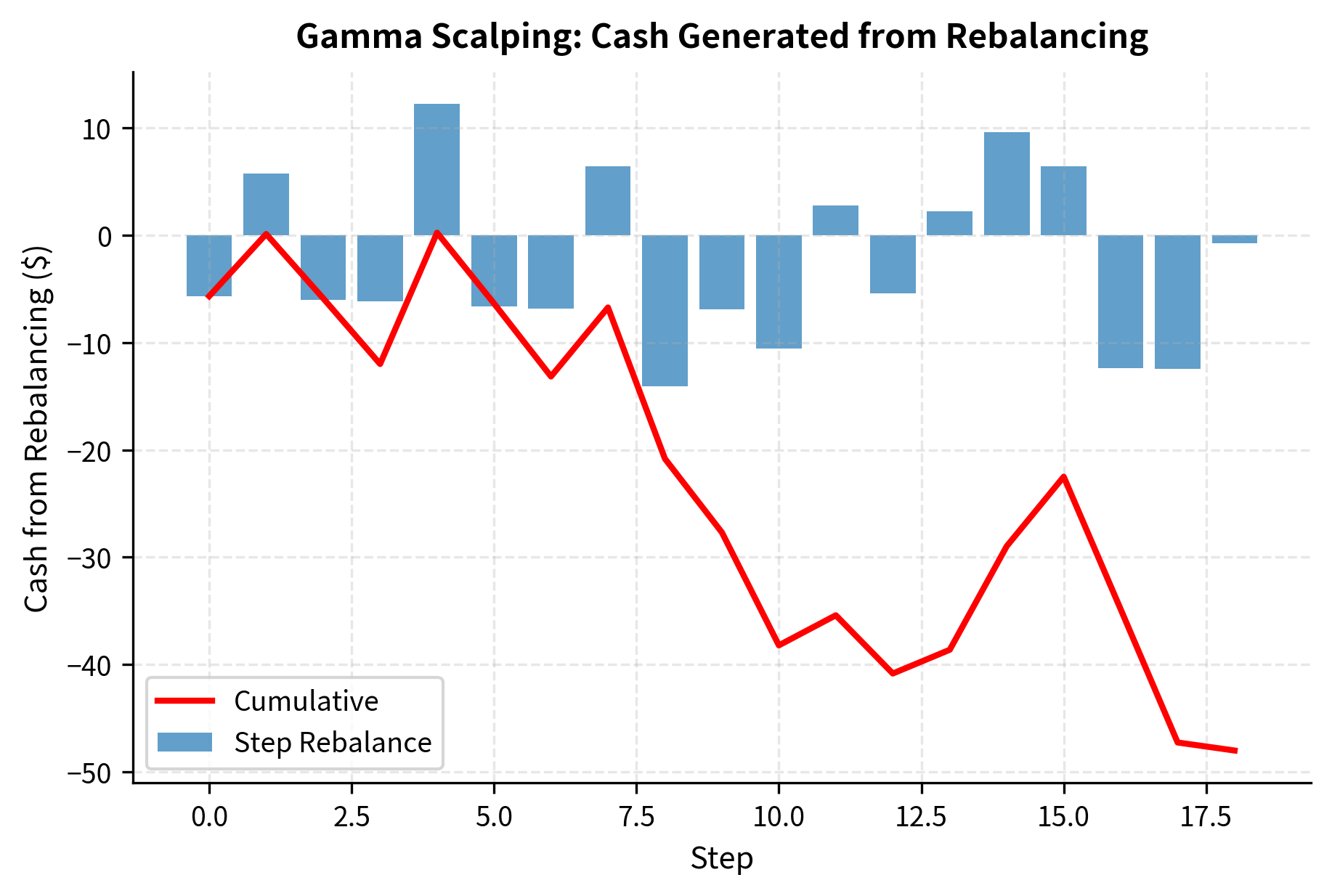
The cash generated from rebalancing must be weighed against the theta decay of the option. If the stock moves enough (high realized volatility), rebalancing profits exceed theta costs, and the long gamma position is profitable. The chart illustrates how each price move generates a rebalancing transaction, and how these transactions accumulate over time. Notice that the cash generated tends to be positive regardless of whether the stock moves up or down: what matters is the magnitude of the move, not its direction. This directional indifference is the hallmark of a pure volatility position.
Key Parameters
The key parameters for delta-hedging strategies are:
- S: Current stock price. The primary driver of option value and delta.
- K: Strike price. Determines the moneyness of the option and gamma concentration.
- T: Time to expiration. Affects theta decay and gamma magnitude.
- r: Risk-free interest rate. Used in the Black-Scholes pricing and carrying cost calculations.
- σ_imp: Implied volatility. Used to price the option and calculate the hedge ratio (delta).
- σ_real: Realized volatility. The actual volatility of the underlying asset that determines rebalancing P&L.
Volatility Arbitrage
Volatility arbitrage strategies seek to profit from differences between implied volatility and expected realized volatility. These strategies require both a view on future volatility and the ability to isolate volatility exposure through hedging. The term "arbitrage" is a misnomer; these strategies involve taking a view rather than exploiting a riskless mispricing. However, the term has become standard in the industry to describe strategies that attempt to profit from the difference between where volatility is priced and where it will actually be realized.
Long Volatility Strategies
You go long volatility when you believe options are underpriced relative to future realized volatility. This typically occurs:
- Before anticipated high-volatility events (earnings, elections, major economic announcements)
- When implied volatility is historically low relative to its own range
- When technical or fundamental factors suggest increased uncertainty
Long volatility positions can be constructed through:
- Straddles: Buy both a call and put at the same strike, profiting from large moves in either direction
- Strangles: Buy an out-of-the-money call and put, cheaper but requiring larger moves
- Delta-hedged long options: Buy options and maintain delta-neutral exposure
A straddle combines a call and a put at the same strike price and expiration, creating a position that profits from any large price move regardless of direction. The maximum loss is limited to the premium paid for both options, which occurs if the underlying closes exactly at the strike at expiration. The trade becomes profitable when the underlying moves far enough from the strike to exceed the total premium paid.
The P&L for a long straddle at expiration is:
where:
- : profit or loss at expiration
- : stock price at expiration
- : strike price
- : premium paid for the call
- : premium paid for the put
The formula captures the essential structure of the straddle: at expiration, exactly one of the two options will be in the money (unless the stock closes precisely at the strike). If the stock is above the strike, the call pays out its intrinsic value while the put expires worthless. If the stock is below the strike, the put pays out while the call expires worthless. The first two terms in the formula calculate these payoffs, and the third term subtracts the cost of establishing the position. For the trade to be profitable, the stock must move far enough that the winning option's payoff exceeds the combined cost of both options.
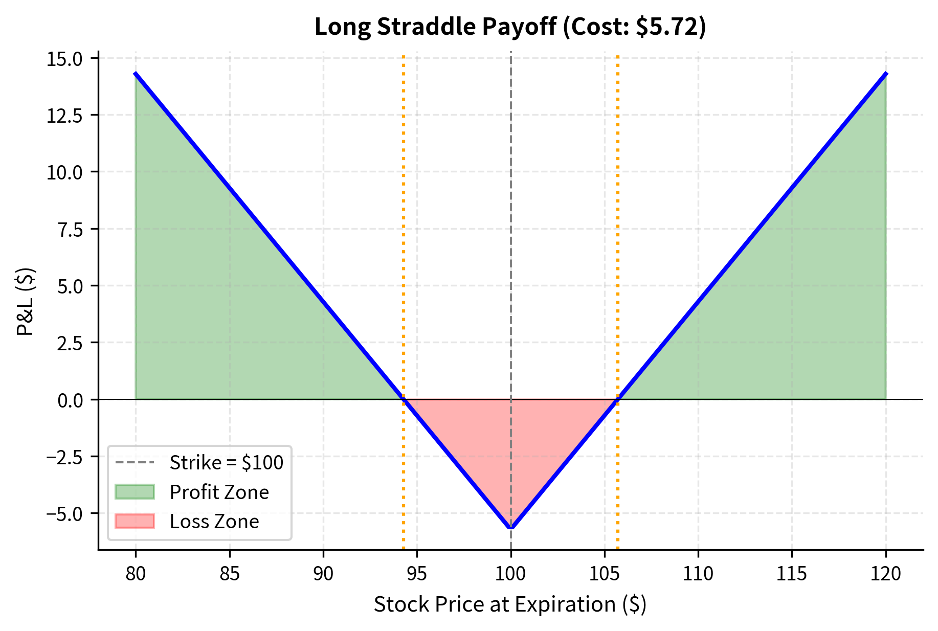
The "implied move" embedded in a straddle price represents the market's expectation of the stock's range. If you believe the stock will move more than this implied amount, you would buy the straddle. This implied move is a convenient way to interpret straddle prices: if a 30-day straddle costs 5% of the stock price, the market is implying that the stock will move approximately 5% in one direction or the other over that period. If you expect the stock to move 8% due to an upcoming catalyst, the straddle looks attractively priced.
Short Volatility Strategies
Short volatility strategies profit when implied volatility exceeds realized volatility. These strategies collect premium from option buyers who overpay for protection. Common approaches include:
- Selling straddles or strangles: Collect premium, profit if stock stays range-bound
- Iron condors: Sell strangle, buy further OTM options for protection
- Covered calls or cash-secured puts: Systematic premium collection
For a short strangle involving a put with strike and a call with strike (where ), the P&L at expiration is:
where:
- : profit or loss at expiration
- : premium received for the put
- : premium received for the call
- : put strike price
- : call strike price
- : stock price at expiration
The formula reveals the risk-reward structure of a short strangle. The first term represents the premium collected upfront, which is the maximum possible profit. This maximum profit is realized if the stock finishes anywhere between the two strikes at expiration, in which case both options expire worthless and you keep the entire premium. The second and third terms represent potential losses: if the stock falls below the put strike or rises above the call strike, you must pay out the intrinsic value of the in-the-money option. Because there is no upper limit to how high the stock can rise and the stock can fall to zero, the potential losses on a short strangle are theoretically unlimited on the upside and substantial on the downside.
The key risk of short volatility strategies is their asymmetric payoff profile. Gains are limited to the premium collected, while losses can be substantial during volatility spikes.
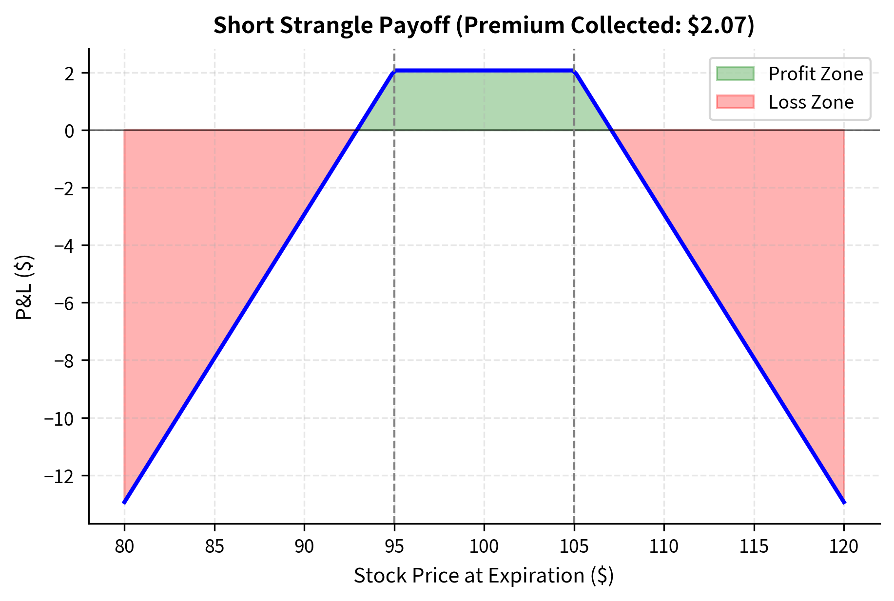
The payoff diagram highlights the defined profit zone between the strikes and the unlimited risk beyond the breakeven points. This structure benefits from time decay but requires the underlying asset to remain within a specific range. The flat profit region in the middle represents the comfort zone for short volatility traders: as long as the stock stays within this range, they earn the full premium. But the steep losses beyond the breakeven points illustrate why risk management is so critical for these strategies.
Building a Volatility Forecast
To succeed at volatility arbitrage, you must predict future realized volatility using one of several approaches:
Historical volatility models estimate future volatility based on past returns. As we covered in Part III, Chapter 18, GARCH models capture volatility clustering and mean reversion. The key insight behind GARCH is that volatility tends to be persistent: high volatility days tend to be followed by high volatility days, and low volatility periods tend to persist as well. By modeling this persistence explicitly, GARCH can provide more accurate short-term volatility forecasts than simple historical measures.
The GARCH forecast differs from the simple historical volatility because it accounts for the recent volatility cluster in the data. By weighing recent observations more heavily and incorporating mean reversion, GARCH models often provide more responsive forecasts than rolling standard deviations. The model recognizes that the recent spike in volatility is likely to persist somewhat into the future, even as it gradually decays back toward the long-run average. This forward-looking adjustment makes GARCH particularly valuable for short-term volatility trading decisions.
Implied volatility models use the term structure and skew of implied volatility to forecast. If short-term implied volatility is elevated relative to longer-term volatility, mean reversion suggests it may decline.
Fundamental factors such as earnings announcements, economic data releases, and geopolitical events can inform volatility expectations.
Key Parameters
The key parameters for volatility forecasting models (like GARCH) are:
- ω (omega): Baseline variance. The long-term floor for volatility.
- α (alpha): Reaction parameter. Determines how much yesterday's shock impacts today's volatility.
- β (beta): Persistence parameter. Determines how long shocks linger in the variance process (memory).
- Returns: The time series of asset returns used to estimate parameters.
Dispersion Trading
Dispersion trading exploits the relationship between index volatility and the volatility of index constituents. The fundamental insight is that index variance depends not only on constituent variances but also on correlations between constituents. When you diversify by combining multiple assets, some of their movements cancel out, reducing overall portfolio volatility. This diversification effect creates a wedge between index volatility and the volatilities of individual stocks, and dispersion trading seeks to profit from this relationship.
The Variance Decomposition
For an index composed of stocks with weights , the index variance is:
where:
- : variance of the index
- : number of stocks in the index
- : weight of stock and in the index
- : volatility of stock and
- : correlation between stocks and
This formula applies portfolio variance mathematics to an index. It tells us that the total variance of the index comes from two distinct sources, and understanding these sources is crucial for dispersion trading.
The formula decomposes index variance into:
- : the weighted sum of individual variances (diagonal terms), representing concentration risk
- : the weighted sum of pair-wise covariances (off-diagonal terms), representing correlation risk
The first component represents what would happen if each stock's movements were entirely independent: you would simply add up the variance contributions from each stock, weighted by the square of their index weights. The second component captures the interaction effects between stocks: when two stocks tend to move together (positive correlation), they add to index variance, while independent or negatively correlated movements partially cancel out.
This can be rewritten using average correlation :
where:
- : variance of the index
- : sum of squared weights (measure of concentration)
- : average variance of constituents
- : average pairwise correlation between constituents
- : square of the average constituent volatility
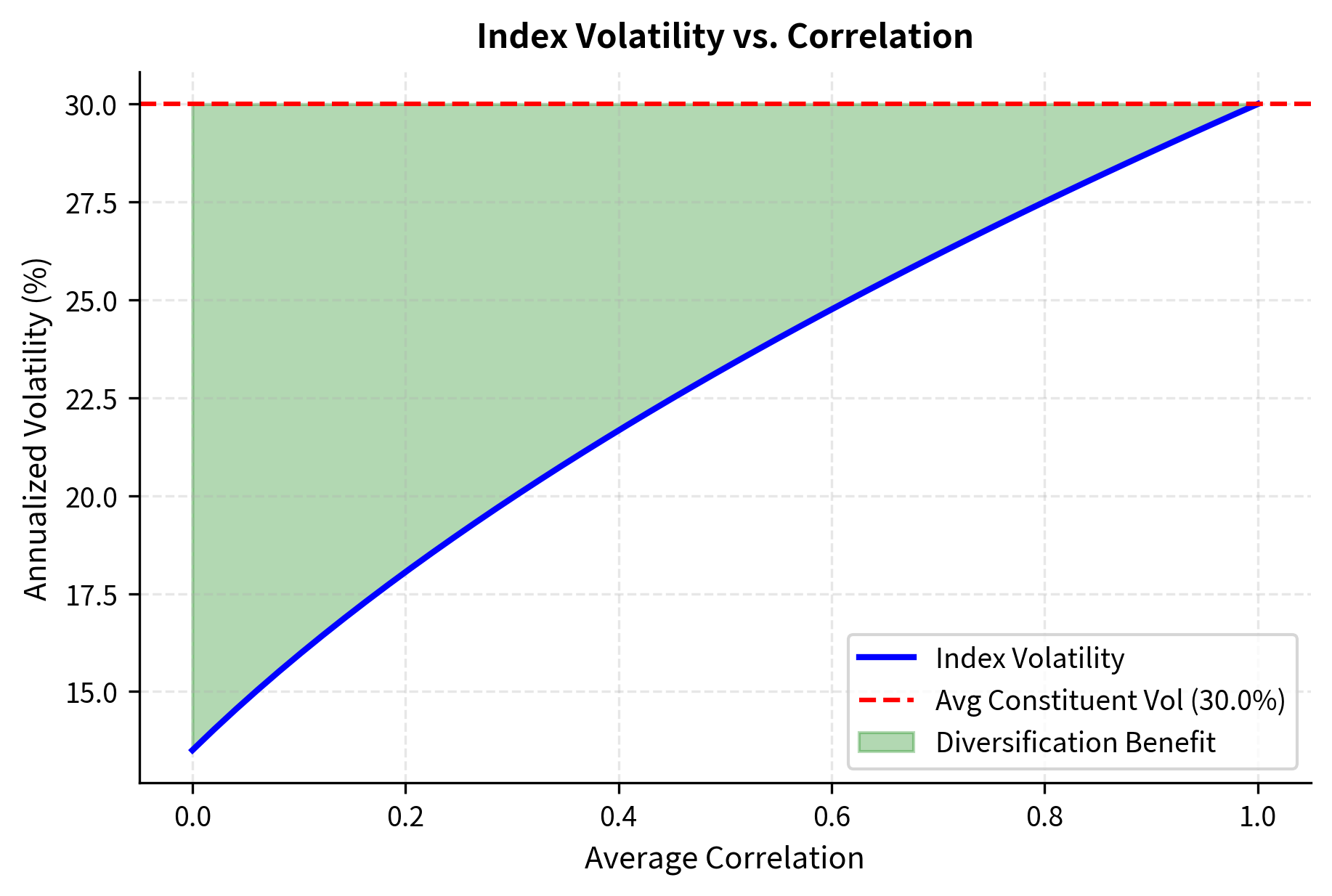
This simplified form makes the role of correlation crystal clear. The first term depends only on individual volatilities and index concentration, while the second term scales directly with the average correlation. When correlation is zero, the second term vanishes entirely, and the index variance is driven purely by the concentration-weighted individual variances. As correlation increases, the second term grows, and the diversification benefit shrinks.
The key implication is that when correlations are high, index volatility approaches the average constituent volatility. When correlations are low, diversification reduces index volatility below constituent volatility.
The Dispersion Trade
A dispersion trade takes opposing volatility positions on an index versus its constituents. The two main configurations are:
Long Dispersion (Short Correlation):
This trade profits when realized correlation is lower than implied correlation. It is typically the direction you choose because implied correlation tends to be higher than realized correlation, similar to the volatility risk premium. Index option buyers are often hedgers who pay a premium for protection against broad market moves. This demand pushes up index implied volatility relative to what the constituent implied volatilities would suggest.
Short Dispersion (Long Correlation):
- Buy index options
- Sell constituent options
This trade profits when correlations spike, typically during market stress. It serves as a tail hedge. During crises, correlations tend to spike as all assets sell off together, causing index volatility to surge relative to individual stock volatilities. A short dispersion position profits from this correlation spike.
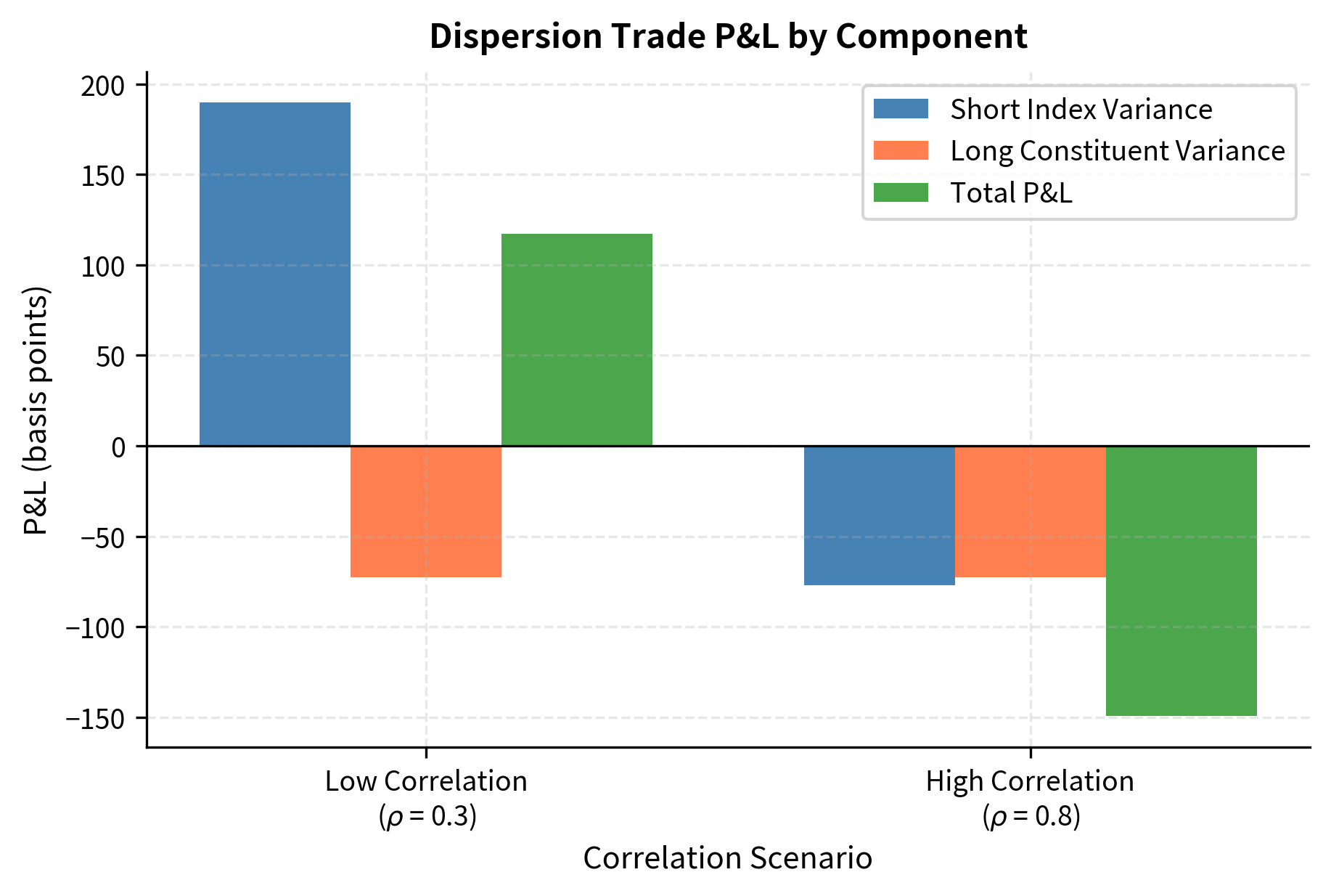
In the low correlation scenario, the realized index volatility is significantly lower than the weighted constituent volatility, generating profit for the dispersion trade (short index, long constituents). When realized correlation is high, this diversification benefit disappears, and the trade suffers losses as the short index position moves against you. The dispersion trade is fundamentally a bet on correlation: if correlations come in lower than what option prices imply, the long dispersion trade profits.
Implied Correlation
You can express your views in terms of implied correlation, which can be backed out from index and constituent implied volatilities:
where:
- : implied correlation derived from market prices
- : implied volatility of the index
- : weights of constituents and
- : implied volatilities of constituents and
This formula inverts the variance decomposition equation to solve for correlation. Given the observed implied volatility of the index and the implied volatilities of all constituents, we can back out the correlation level that would make these prices consistent. This implied correlation represents the market's collective expectation of how correlated stock returns will be over the option's life.
When implied correlation is high relative to expected realized correlation, a long dispersion trade (short correlation) is attractive. You are effectively betting that the market is overpricing co-movement and that individual stocks will move more independently than option prices suggest.
Key Parameters
The key parameters for dispersion trading are:
- w_i: Weight of each constituent in the index.
- σ_index: Volatility of the index. Lower than average constituent volatility due to diversification.
- σ_constituent: Volatility of individual stocks in the index.
- ρ (rho): Pairwise correlation between constituents. The primary driver of the spread between index and constituent volatility.
The implied correlation of 0.25 indicates that the market is pricing in a relatively low level of co-movement between stocks. If you believe actual correlation will be higher, you might sell dispersion (buy index options, sell constituent options).
Variance Swaps
Variance swaps are derivatives that provide pure exposure to realized variance, making them a cleaner instrument for volatility trading than delta-hedged options. Unlike options, which have path-dependent Greeks that require continuous hedging, variance swaps pay off directly based on the total realized variance over their life. This simplicity makes them attractive for you if you want volatility exposure without the operational complexity of dynamic hedging.
Structure and Payoff
A variance swap is a forward contract on realized variance. At maturity, the payoff is:
where:
- : payment received at maturity
- : variance notional (typically quoted as vega notional divided by )
- : annualized realized variance over the swap's life
- : variance strike (typically expressed as volatility: )
The payoff formula is simple. You receive a payment proportional to the difference between actual realized variance and a predetermined strike level. If the market is more volatile than the strike implies, you profit. If the market is calmer than expected, you pay the seller. Unlike options, there is no optionality here: the trade settles purely based on what happens to variance, with no path dependence in terms of when or how the moves occur.
The realized variance is calculated from daily log returns:
where:
- : number of observation days
- : price of the asset on day
- : price of the asset on day
- : annualization factor (assuming trading days)
Note that this formula uses the sum of squared returns directly, not the variance around the mean. This is the standard market convention and ensures the calculation is path-dependent and captures all price movements. The distinction matters: by using squared returns rather than variance around the mean, the calculation captures both the variance and any drift in the returns. This convention means that a market that trends strongly in one direction will register higher "realized variance" than one that fluctuates around a stable level, even if the two have identical standard deviations. This feature makes variance swaps sensitive to all price movements, not just deviations from trend.
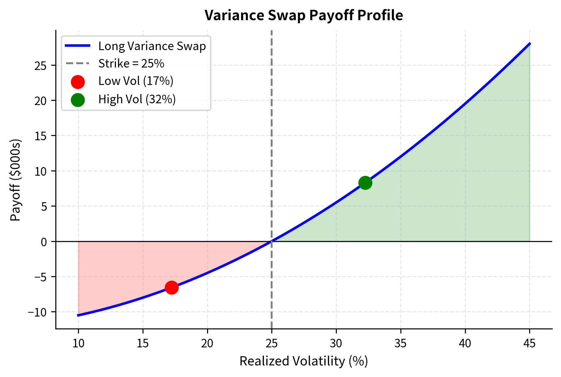
The variance swap generates a positive payoff when realized volatility exceeds the strike volatility. Note that in the high volatility scenario, the payoff is substantial because the realized variance (volatility squared) increases quadratically, making the payout convex with respect to volatility moves. This convexity is a critical feature of variance swaps: a move from 25% to 35% volatility generates more profit than a move from 25% to 15% volatility generates loss, making variance swaps attractive instruments for long volatility positions.
Replication and Pricing
The variance swap strike is determined by a portfolio of options across all strikes. The theoretical result, derived by Demeterfi, Derman, Kamal, and Zou (1999), shows that variance can be replicated by a portfolio of options with weights inversely proportional to the square of the strike:
where:
- : variance strike
- : risk-free interest rate
- : time to expiration
- : forward price of the underlying asset
- : strike price
- : price of a put option with strike
- : price of a call option with strike
Variance exposure can be constructed from a portfolio of vanilla options. The key insight is that options at different strikes contribute differently to variance: lower strike options contribute more (because of the weighting) than higher strike options. This overweighting of low strikes reflects the fact that the logarithm function used in variance calculation is more sensitive to downward price moves than upward ones.
The formula splits the replication into two parts based on the forward price :
- : replicates variance using out-of-the-money puts for strikes below the forward price
- : replicates variance using out-of-the-money calls for strikes above the forward price
Using out-of-the-money options at each strike is a convention that minimizes the cost of maintaining the replicating portfolio, as OTM options have lower premiums than their in-the-money counterparts while providing the same exposure to variance.
In practice, this integral is approximated using available option strikes:
The variance swap fair strike is typically slightly higher than at-the-money implied volatility due to the convexity in the variance payoff. This convexity adjustment compensates for the asymmetric exposure to volatility: realized variance of 40% versus 20% strike creates more P&L than 20% versus 20%. The convexity adjustment exists because variance is the square of volatility: a symmetrical distribution of volatility outcomes translates into an asymmetrical distribution of variance outcomes, with large volatility outcomes contributing disproportionately to expected variance.
Vega Notional Versus Variance Notional
Variance swaps can be quoted in two ways:
Variance notional (): The dollar amount paid per point of variance. A variance notional of $1,000 pays $1,000 for each 0.0001 (1 bp) difference in variance.
Vega notional: The approximate P&L for a 1 percentage point change in volatility. For a vega notional of $100,000, if volatility moves from 25% to 26%, the P&L is approximately $100,000.
The relationship between them is:
where:
- : variance notional
- : vega notional (P&L per 1 vol point change)
- : volatility strike
This conversion is approximate because the variance payoff is convex in volatility. The formula comes from taking the derivative of variance with respect to volatility at the strike level: the derivative of with respect to is , so at the strike volatility , a small change in volatility creates a variance change of approximately times the volatility change. The vega notional convention makes it easier for you to think in terms of volatility points, which are more intuitive than variance points.
Key Parameters
The key parameters for variance swaps are:
- K_vol: Volatility strike. The reference level of volatility; payoff is zero if realized volatility equals this strike.
- N_vega: Vega notional. The approximate P&L per 1% change in volatility.
- Realized Variance: The sum of squared daily log returns over the life of the contract, annualized.
Trading the VIX
The CBOE Volatility Index (VIX) provides a benchmark for S&P 500 implied volatility. VIX derivatives, such as futures and options, allow you to take positions on volatility expectations and hedge volatility risk.
VIX Calculation
The VIX is calculated from a portfolio of S&P 500 index options using a methodology similar to variance swap pricing. It represents the 30-day expected volatility implied by option prices:
where:
- : variance used to calculate VIX ()
- : time to expiration
- : interval between strike prices
- : strike price of the -th option
- : risk-free interest rate
- : midpoint of the bid-ask spread for option at strike
- : forward index level derived from option prices
- : first strike below the forward price
The VIX calculation methodology is directly related to the variance swap replication formula we examined earlier. Both approaches use a portfolio of out-of-the-money options weighted by the inverse square of the strike to capture expected variance. The key difference is that the VIX uses a specific set of S&P 500 options with near-term and next-term expirations, interpolated to provide a constant 30-day horizon.
The formula consists of two main parts:
- Option Summation: aggregates the prices of out-of-the-money options, weighted by , to replicate the variance payoff.
- Forward Adjustment: corrects for the discrete difference between the forward price and the cutoff strike .
The forward adjustment term is necessary because the formula uses a discrete set of option strikes rather than a continuous spectrum. Since the transition between puts and calls occurs at rather than exactly at the forward price , this adjustment corrects for the small pricing error that would otherwise result.
VIX Futures Term Structure
VIX futures prices reflect expectations of future VIX levels plus a risk premium. The typical term structure shapes are:
- Contango: Normal market conditions. Longer-dated futures trade above spot VIX because investors demand premium for bearing volatility risk.
- Backwardation: Market stress periods. Spot VIX spikes above futures as realized volatility jumps and mean reversion is expected.
The intuition for contango is similar to the volatility risk premium. Investors who are long equity portfolios want protection against volatility spikes, and they are willing to pay a premium for this protection. VIX futures sellers, who bear the risk of volatility spikes, demand compensation in the form of futures prices that are higher than expected future spot VIX levels. This premium manifests as an upward-sloping term structure.
During market stress, the relationship inverts. When volatility spikes, the spot VIX jumps immediately to reflect current fear and hedging demand. However, futures prices rise less because the market expects volatility to eventually mean-revert to more normal levels. This creates backwardation, with spot VIX above futures prices.
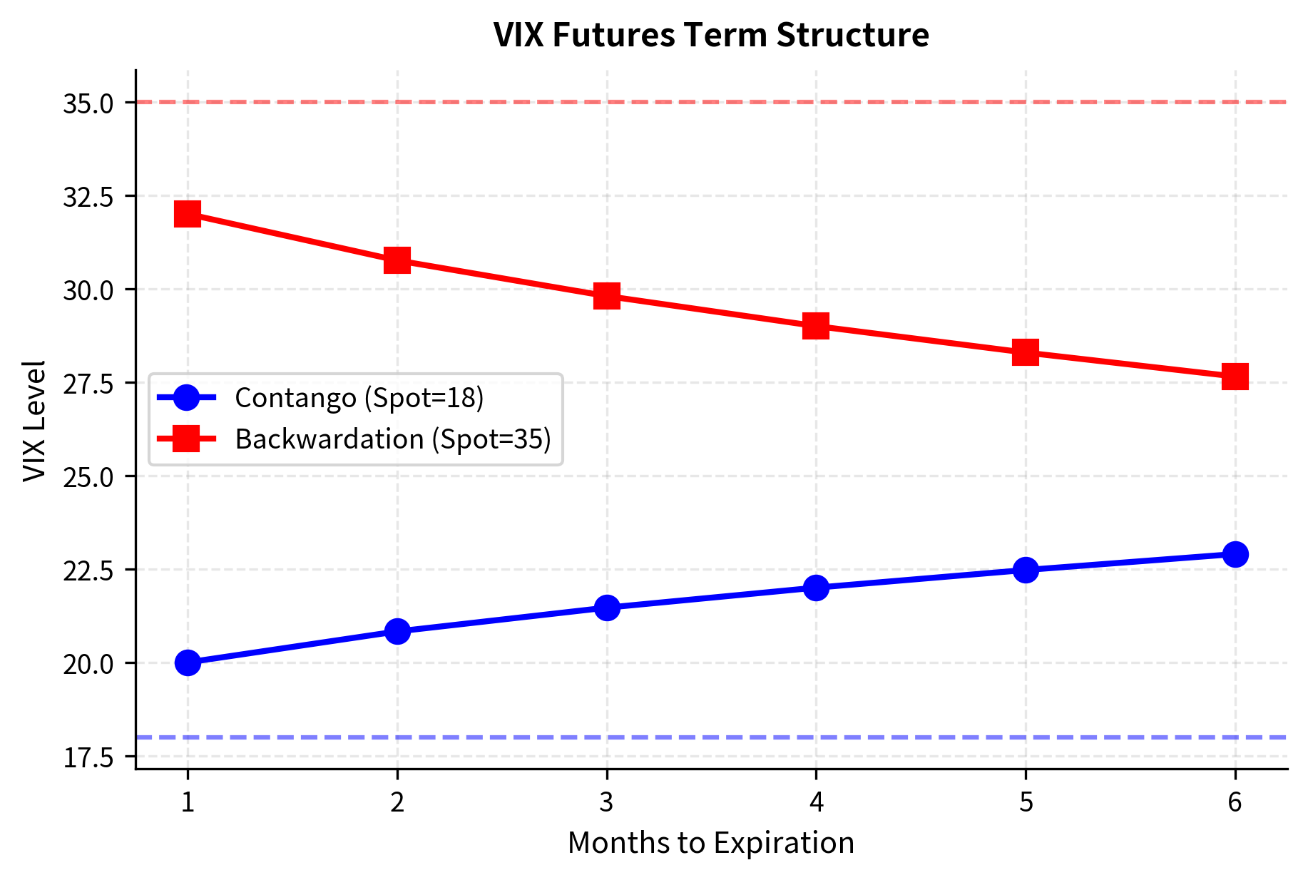
The term structure typically exhibits contango, where longer-dated futures trade at a premium to spot, reflecting the cost of protection. During market stress, the curve flips to backwardation, with spot prices surging above futures as demand for immediate hedging spikes.
Roll Yield and VIX Products
The persistent contango in VIX futures creates a negative roll yield for long positions. As futures converge to spot at expiration, long positions in contango lose value from roll. This explains why long VIX ETFs like VXX have lost over 99% of their value since inception, despite VIX remaining in a range.
This decay is devastating for long-term holders. Consider a VIX ETF that maintains exposure to the front-month VIX futures contract. When the contract approaches expiration, the ETF must roll its position to the next month's contract. If the curve is in contango, this means selling the expiring contract at a lower price and buying the next month's contract at a higher price. This roll transaction locks in a loss, and if contango persists, these losses accumulate month after month, steadily eroding the ETF's value.
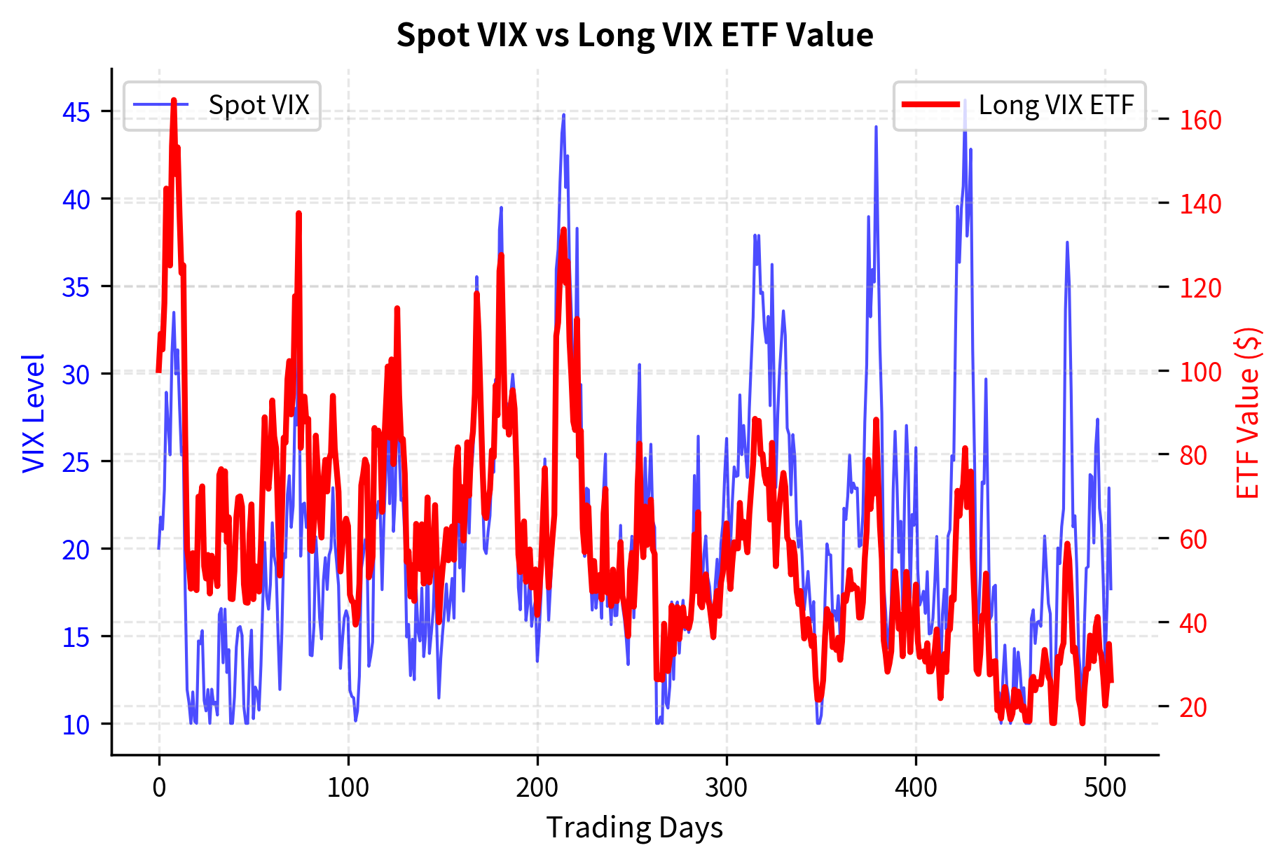
The lesson is clear: long volatility positions using VIX products require precise timing. They are hedging instruments, not investments.
Key Parameters
The key parameters for VIX products are:
- Spot VIX: The current level of the VIX index, representing 30-day implied volatility.
- Roll Yield: The cost incurred from rolling futures contracts. Negative in contango, positive in backwardation.
- Term Structure: The curve of futures prices across maturities. Shape determines the cost of carry.
- Contango: Market condition where futures prices exceed spot prices, typical for VIX.
Risks of Volatility Trading
Volatility trading risks differ from directional equity or fixed income strategies. Understanding these risks is essential for proper position sizing and risk management.
Short Volatility Risk: The Picking Up Nickels Problem
Short volatility strategies typically produce frequent small gains and occasional large losses. This profile resembles "picking up nickels in front of a steamroller"; the strategy works until it doesn't.
The danger stems from several factors. Volatility is inherently mean-reverting but can spike dramatically and persistently during market stress. Historical examples include the 2008 financial crisis, the 2015 Chinese market turmoil, and the February 2018 "Volmageddon" event when inverse VIX products collapsed overnight. During Volmageddon, the VIX doubled in a single day, causing the XIV ETN (which sold VIX futures) to lose 90% of its value and be liquidated.
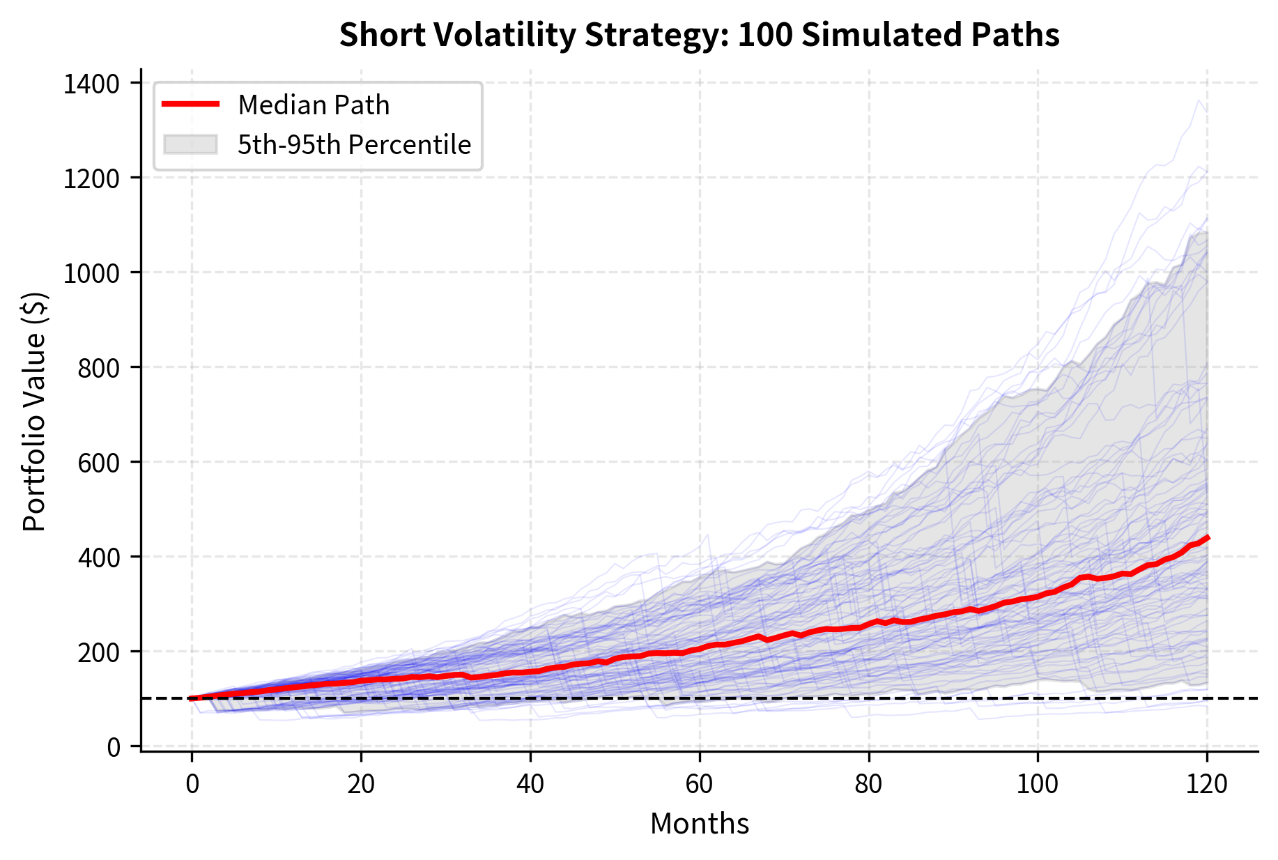
The simulation demonstrates the 'tail risk' inherent in short volatility strategies. While the median path is profitable, the presence of ruinous drawdowns and high probabilities of significant loss illustrates why simple historical mean returns can be misleading for risk assessment in volatility markets.
Long Volatility Risk: The Carry Problem
Long volatility strategies face the opposite challenge: they tend to lose money slowly through carry costs but profit during volatility events. The volatility risk premium means implied volatility typically exceeds realized volatility, creating a drag on long vol positions.
The carry cost manifests in several ways:
- Theta decay: Long options value daily, requiring volatility events to offset
- Roll yield: Long VIX futures contango lose money as they converge to spot
- Variance swap negative carry: Buying variance swaps elevated implied levels loses if realized vol is lower
The behavioral challenge for you is maintaining conviction through extended periods of losses while waiting for the volatility event that justifies the strategy.
Position Sizing and Leverage
Position sizing is critical because of these asymmetric risk profiles:
For short volatility: You should size positions to survive 3-4 standard deviation moves. The February 2018 VIX spike was approximately a 7-sigma event under normal assumptions, highlighting the inadequacy of normal distribution assumptions. For long volatility: You should size positions to survive extended carry costs. A long vol strategy might need to withstand 12-24 months of bleeding before a payoff event occurs.
A useful framework is for you to define the maximum acceptable drawdown and work backward to position size:
This position size ensures that a 40% loss in a volatility spike does not exceed the 15% drawdown limit. This inverse sizing approach is crucial for survival in fat-tailed markets.
Correlation with Market Stress
Volatility positions have distinct correlation properties that affect portfolio construction:
- Short volatility is implicitly long equities. When markets crash, volatility spikes, and short vol positions lose money at the worst time.
- Long volatility provides crisis alpha: profits during market stress that can offset equity losses.
This correlation structure means that short volatility strategies provide false diversification. They may show low correlation to equities during calm periods but become highly correlated during crises when diversification is most needed.
Practical Implementation Considerations
Quiz
Ready to test your understanding? Take this quick quiz to reinforce what you've learned about volatility trading and arbitrage strategies.

Comments